Evolution of the Cluster X-ray Luminosity Function

Abstract

We report measurements of the cluster X-ray luminosity function out to $z=0.8$ based on the final sample of 201 galaxy systems from the 160 Square Degree ROSAT Cluster Survey. There is little evidence for any measurable change in cluster abundance out to $z\sim 0.6$ at luminosities less than a few times 10⁴⁴ $h_{50}^{-2}$ ergs s^-1 (0.5–2.0 keV). However, between $0.6<z<0.8$ and at luminosities above 10⁴⁴ $h_{50}^{-2}$ ergs s^-1, the observed volume densities are significantly lower than those of the present-day population. We quantify this cluster deficit using integrated number counts and a maximum-likelihood analysis of the observed luminosity-redshift distribution fit with a model luminosity function. The negative evolution signal is $>3\sigma$ regardless of the adopted local luminosity function or cosmological framework. Our results and those from several other surveys independently confirm the presence of evolution. Whereas the bulk of the cluster population does not evolve, the most luminous and presumably most massive structures evolve appreciably between $z=0.8$ and the present. Interpreted in the context of hierarchical structure formation, we are probing sufficiently large mass aggregations at sufficiently early times in cosmological history where the Universe has yet to assemble these clusters to present-day volume densities.

1. Introduction

Galaxy clusters form via the gravitational amplification of rare, high peaks in the cosmic matter density field. The redshift evolution of cluster abundance depends on the growth rate of density perturbations which is, in turn, sensitive to the mean cosmic matter density ($\Omega_{M}$) and, to a lesser extent, the dark-energy density ($\Omega_{\Lambda}$). Thus observations of cluster space density with sufficient temporal sampling can provide powerful cosmological constraints (e.g., Oukbir & Blanchard, 1992; Eke et al., 1998; Bahcall et al., 1999).

A directly measurable and robust diagnostic of cluster abundance is the X-ray luminosity function (XLF), that is the volume density of clusters per luminosity interval. X-ray selected galaxy clusters are particularly well-suited for this type of analysis. Clusters are efficiently detected at X-ray wavelengths to high redshift (currently out to $z\sim 1.25$) thus providing the leverage for evolutionary studies (see review by Rosati, Borgani, & Norman, 2002). The resulting samples feature high statistical completeness which is clearly important for deriving reliable number counts. Since X-ray surveys have well-defined selection functions, it is straight-forward to convert these number counts into volume-normalized measures such as the luminosity function. Finally, given the strong correlation between X-ray luminosity and cluster mass, it is possible to transform the observed XLF into the cluster mass function which is the fundamental relation in the theoretical treatment.

Though the cluster XLF was first measured with an X-ray flux-limited sample over two decades ago (Piccinotti et al., 1982), a definitive characterization of its evolution has proven very difficult. The latter is a particularly important test in observational cosmology because the variation of the cluster XLF as a function of redshift reflects the evolution of the cluster mass function. Such a measure allows for strong constraints on $\Omega_{M}$ even accounting for uncertainty in the luminosity-mass relation (e.g., Borgani et al., 2001). Early theoretical predictions (e.g., Kaiser, 1986) postulated dramatic positive evolution in the XLF where the volume density of clusters of a fixed luminosity would increase with redshift. This would be an “observer-friendly” universe since the loss in sensitivity at high redshift in a flux-limited survey would be offset by the growing population of detectable sources. Contrary to this scenario, observations of the cluster XLF range from zero evolution to negative evolution depending on the redshifts and luminosities probed. These findings are consistent with current predictions for a low-density universe where mild negative evolution is restricted to the most luminous, high-redshift clusters while there is little change in the bulk of the population (e.g., Borgani & Guzzo, 2001, and references therein).

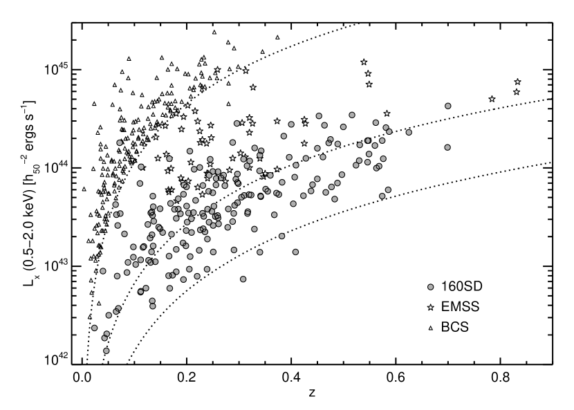
Figure 1.— X-ray luminosity and redshift distribution of the 160SD (Mullis et al., 2003), the EMSS (Gioia & Luppino 1994 with updates from the literature, e.g., Henry 2000), and the BCS (Ebeling et al., 1998) cluster samples. The dotted curves (left to right) are indicative flux limits of 2.7 $\times$ 10^-12, 1.5 $\times$ 10^-13, and 3 $\times$ 10^-14 ergs cm^-2 s^-1 (0.5–2.0 keV). The EMSS and BCS luminosities were converted to this energy band assuming a Raymond-Smith plasma spectrum (Raymond & Smith, 1977) with a metallicity of 0.3 solar and the reported gas temperature (either directly measured or estimated from the luminosity-temperature relation).

Taking advantage of the first time an X-ray survey extended into cosmologically interesting redshifts, Gioia et al. (1990a) and Henry et al. (1992) used 67 clusters ($0.14<z<0.60$) from the pioneering Einstein Extended Medium Sensitivity Survey (EMSS; Gioia et al., 1990b; Stocke et al., 1991; Maccacaro et al., 1994) to make the first detection of evolution in the observed XLF. Based on a steepening of the high-redshift luminosity function, they found a deficit of high-luminosity clusters at $z>0.3$ with a statistical significance of approximately 3$\sigma$. Though most subsequent investigations corroborate these findings, some questions have been raised concerning the reliability of the EMSS evolution detection (e.g., Nichol et al., 1997; Ebeling et al., 2000b; Ellis & Jones, 2002; Lewis et al., 2002). Of historical note, the only other pre-ROSAT measurement of significant cluster evolution came from Edge et al. (1990) who found rapid negative evolution in the luminosity function at $z<0.2$ based on a HEAO-1 sample. This was ultimately overruled by a definitive and non-evolving measure of the local XLF (Ebeling et al., 1997).

Seeking in part to confirm or refute the EMSS’s controversial claim of negative cluster evolution, a large number of cluster surveys were initiated in the 1990s based on ROSAT data (Voges, 1992; Trümper, 1993). The 160 Square Degree ROSAT Cluster Survey (hereafter 160SD, Vikhlinin et al., 1998a; Mullis et al., 2003) is one such program and the subject of this paper. Additional surveys probing to high redshift include the NEP (Mullis, 2001; Henry et al., 2001; Gioia et al., 2003), BMW-HRI (Moretti et al., 2001; Panzera et al., 2003), BSHARC (Romer et al., 2000), MACS (Ebeling, Edge, & Henry, 2001), RDCS (Rosati et al., 1995, 1998, 2000), RIXOS (Castander et al., 1995; Mason et al., 2000), SSHARC (Burke et al., 2003), and WARPS (Scharf et al., 1997; Perlman et al., 2002). Complementary surveys at low redshifts ($z\lesssim 0.3$) yielded accurate determinations of the local luminosity function, thus providing the crucial baseline for the detection of redshift evolution. These local surveys include the BCS+eBCS (Ebeling et al., 1998, 2000a), RASS1BS (De Grandi et al., 1999a), and REFLEX (Böhringer et al., 2001). From the shear number of projects it should be clear that ROSAT was a watershed event for X-ray cluster surveys.

Critical comparisons of the ROSAT and EMSS luminosity functions must account for the overlap (or lack thereof) of the measurements in redshift and luminosity. Insufficient attention to this point led to confusion in some early analyses and debates. Different combinations of sensitivity and areal coverage in flux-limited surveys, when convolved with the intrinsic cluster luminosity function, result in populating different regions of the observed luminosity-redshift plane (see indicative results in Figure 1). In practice it is difficult to directly test the cluster evolution seen in the EMSS detection because it lies at the extreme bright end of the luminosity function. Thus large search volumes are required to detect adequate numbers of such rare clusters. The 160SD is one of the largest serendipitous X-ray surveys conducted with ROSAT. With this substantial areal coverage and high sensitivity, the 160SD survey is well-positioned to probe cluster evolution. Preliminary analyses of our sample, with at-the-time incomplete optical follow-up, seemed to confirm the deficit of high-luminosity, high-redshift clusters first seen by the EMSS (Vikhlinin et al., 1998b, 2000).

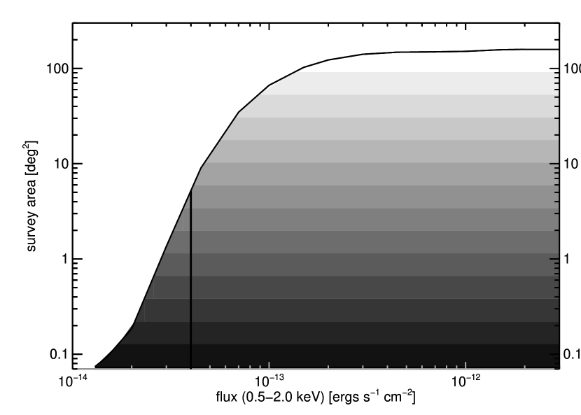
Figure 2.— The selection function of the 160SD survey specifying the square degrees of area covered as a function of limiting X-ray flux (0.5–2.0 keV). These data are tabulated in Vikhlinin et al. (1998a, Table 5). The shading encodes this information for subsequent use in Figure 3. The vertical line indicates the minimum flux limit (4 $\times$ 10^-14 ergs cm^-2 s^-1, 0.5–2.0 keV) used in the present analysis.

In this paper we present measurements of the cluster XLF out to $z=0.8$ and describe their implications for cluster evolution based on the final 160SD sample of 201 clusters. In § 2 we outline the basic construction of our cluster sample and the associated selection function used herein. The formalism associated with the XLF is defined in § 3 and used to measure cluster abundances at both low and high redshifts. In § 4 we characterize the evolution in the cluster population using integrated number counts and a maximum-likelihood analysis of the observed luminosity-redshift distribution relative to an evolving Schechter function. We discuss our results in the context of previous works and draw conclusions in § 5. Throughout this analysis we use the cosmological parameters $H_{0}=50$ h₅₀ km s^-1 Mpc^-1, $\Omega_{M}=1$, and $\Omega_{\Lambda}=0$ (Einstein–de-Sitter, EdS) for direct comparison to previous work in this field. We also repeat calculations in the currently preferred cosmology where $\Omega_{M}=0.3$ and $\Omega_{\Lambda}=0.7$. X-ray fluxes and restframe luminosities are quoted in the 0.5–2.0 keV energy band unless otherwise stated.

2. The 160SD Cluster Sample

The 160SD sample of 201 galaxy clusters is the largest high-redshift, X-ray selected sample published so far. For instance, there are 73 objects at $z>0.3$ and 22 objects at $z>0.5$. The 160SD sample was constructed via the serendipitous detection of extended X-ray sources in 647 archival ROSAT PSPC observations. Of 223 cluster candidates, we identified 201 as galaxy clusters, 21 as probable false-detections due to blends of unresolved point sources, and one source is unidentified due to its proximity to a bright star. We have secured spectroscopic redshifts for 200 of the 201 clusters. Vikhlinin et al. (1998a) give a complete description of the survey methodology. Mullis et al. (2003) detail the optical follow-up and present the final cluster catalog with spectroscopic redshifts. Note that the number of false-detections in the sample agrees very well with that expected from the confusion of point sources as demonstrated in the Monte-Carlo simulations of Vikhlinin et al. (1998a). Two false-detections (Nos. 77 and 141) serendipitously imaged by XMM-Newton and Chandra, respectively, are indeed confused point sources. Finally, the optical survey imaging was sufficiently deep to demonstrate that none of the false-detections should be galaxy clusters at $z\lesssim 0.9$.

Although spatial X-ray extent was our primary selection criterion, detailed comparisons with other surveys demonstrate that no known clusters were missed as unresolved sources (see § 4 of Mullis et al., 2003, and references therein). Thus the 160SD clusters are in effect drawn from a statistically complete, flux-limited survey with an areal coverage ($\Omega$) and sensitivity characterized by the selection function shown in Figure 2. A total of 158.5 deg² were surveyed and the median survey flux (where $\Omega=\Omega_{\rm total}/2$) is 1.2 $\times$ 10^-13 ergs cm^-2 s^-1 (0.5–2.0 keV). We restrict our analysis to a minimum flux of  4 $\times$ 10^-14 ergs cm^-2 s^-1  to avoid any uncertainties in the sky coverage at very faint fluxes. There are 190 clusters in the 160SD survey sample above this flux limit. Figure 1 shows the position in luminosity-redshift space of our sample relative to the BCS, one of the key reference samples at low redshift, and the EMSS. Figure 3 shows the 160SD data in greater detail. Here the cluster luminosities are plotted as a linear function of comoving volume which provides a more uniform view of the volume sampling. The greyscale in the figure indicates the parameter space probed by our survey — sensitivity is maximal in light regions and minimal in dark regions.

In our subsequent derivations of the cluster XLF and tests for evolution, we exclude several objects (all at $z<0.3$) to minimize the biasing of our results. To avoid potentially skewing the impartiality of the sampling, we reject nine clusters whose redshifts are within $\Delta z=0.015$ of the original target of the ROSAT PSPC observations (Nos. 16, 32, 112, 134, 165, 166, 174, 177, 206). Four X-ray-overluminous elliptical galaxies or “fossil groups” (Nos. 110, 144, 201, and 211) are discounted because these special structures are unlikely to meet the selection criteria of the local samples (Vikhlinin et al., 1999). Thus the final cluster sample used here consists of 177 clusters.

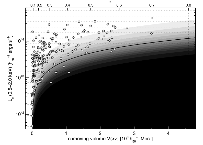
Figure 3.— X-ray luminosity of the 160SD clusters versus redshift $z$ (top axis) and comoving volume out to redshift $z$ (bottom axis). The volume corresponds to a survey solid angle of 158.5 deg² in an Einstein–de-Sitter cosmology. The shading, established in Figure 2, demonstrates the range of survey flux limits and associated sky coverage in this parameter space. The thick, solid curve indicates the minimum flux limit (4 $\times$ 10^-14 ergs cm^-2 s^-1, 0.5–2.0 keV) used in the present analysis. The horizontal (vertical) dashed lines are the boundaries of the luminosity (redshift) bins used in computing the luminosity function.

3. The X-ray Luminosity Function

We define the cluster differential luminosity function to be

$$\phi(L_{\rm X},z)~{}=\frac{d^{2}N}{dVdL_{\rm X}}(L_{\rm X},z)$$ (1)

where $N$ is the number of clusters of luminosity $L_{\rm X}$ in a volume $V$ at a redshift $z$. The standard approach for deriving a nonparametric representation of the differential cluster XLF is based on the $1/V_{\rm max}$ technique first proposed by Schmidt (1968) and generalized by Avni & Bahcall (1980). Here the observed luminosity range is parsed into bins of width $\Delta L$, within each of which there are $N_{j}$ observed clusters. The XLF is estimated by summing the density contributions of each cluster in the considered luminosity/redshift bin,

$$\phi(L_{{\rm X}},z)~{}=~{}\frac{1}{\Delta L}\sum_{i=1}^{N_{j}}~{}\frac{1}{V_{\rm max}(L_{{\rm X},i})~{}},$$ (2)

where $V_{\rm max}$ is the total comoving volume in which a cluster of luminosity $L_{{\rm X},i}$ could have been detected above the flux limits of the survey. Over a specific redshift interval ($z_{\rm min}<z<z_{\rm max}$), this search volume is defined to be

$$V_{\rm max}(L_{\rm X})~{}=~{}\int_{z_{\rm min}}^{z_{\rm max}}\Omega(f_{\rm X}(L_{\rm X},z))~{}\frac{dV(z)}{dz}~{}dz.$$ (3)

Here $\Omega(f_{\rm X})$ is the sky area surveyed in steradians as a function of X-ray flux and $\frac{dV(z)}{dz}$ is the differential, comoving volume element per steradian.

Page & Carrera (2000) describe a refinement to the canonical approach in which the estimator takes the form

$$\phi(L_{{\rm X}},z)~{}=~{}\frac{N_{j}}{\int_{L_{\rm X,min}}^{L_{\rm X,max}}\int_{z_{\rm min}}^{z_{\rm max}}\Omega(f_{\rm X}(L_{\rm X},z))~{}\frac{dV(z)}{dz}~{}dz~{}dL_{\rm X}}$$ (4)

where the boundaries of the luminosity bin are specified by $L_{\rm X,min}$ and $L_{\rm X,max}$. The effect of bringing the luminosity interval into the double integral results in a better estimate of the effective $\Delta L$ which can be smaller than the full bin width for regions of luminosity-redshift space transected by the survey flux limit (e.g., faint luminosities). We will use the Page-Carrera (PC) estimator in our subsequent derivations of the cluster XLF. However, the results are essentially identical to the classical $1/V{\rm max}$ procedure except at the very faint end where the XLF is marginally increased.

As for a parametric representation of the cluster XLF, observations are well fit by a Schechter function (Schechter, 1976) of the form

$$\phi(L_{{\rm X}},z)\,dL_{\rm X}~{}=~{}\phi^{\star}\left(\frac{L_{\rm X}}{L_{\rm X}^{\star}}\right)^{-\alpha}\exp\left(-\frac{L_{\rm X}}{L_{\rm X}^{\star}}\right)\frac{dL_{\rm X}}{L_{\rm X}^{\star}}$$ (5)

where $\phi^{\star}$ is the normalization (units $h_{50}^{3}$ Mpc^-3), $\alpha$ is the faint-end slope, and $L_{\rm X}^{\star}$ is the characteristic luminosity marking the interface between the power-law and the exponential regimes. An equivalent expression for the XLF commonly used in the literature is

$$\phi(L_{{\rm X}},z)\,~{}=~{}{\cal A}\,L_{\rm X}^{-\alpha}\exp\left(-\frac{L_{\rm X}}{L_{\rm X}^{\star}}\right).$$ (6)

With $L_{\rm X}$ in units of 10⁴⁴ $h_{50}^{-2}$ ergs s^-1, the associated normalization, ${\cal A}$, has units of $h_{50}^{3}$ Mpc^-3 (10⁴⁴ $h_{50}^{-2}$ ergs s^-1)^α-1, and the two normalizations are related by $\phi^{\star}\,=\,{\cal A}\,(L_{\rm X}^{\star})^{1-\alpha}$.

Table 1Best-Fit Schechter Parameters for the Local Cluster XLF ($z<0.3$)

Sample	$L_{\rm X}^{\star}$	$\alpha$	$\phi^{\star}$	Reference
	($10^{44}$ $h_{50}^{-2}$ ergs s-1)		$h_{50}^{3}$ Mpc-3
BCS	$5.70^{+1.29}_{-0.93}$	$1.85^{+0.09}_{-0.09}$	($7.56^{+0.82}_{-0.75}$) $\times$ 10-8	Ebeling et al. (1997)
RASS1BS	$3.80^{+0.70}_{-0.55}$	$1.52^{+0.11}_{-0.11}$	($2.53^{+0.22}_{-0.22}$) $\times$ 10-7	De Grandi et al. (1999b)
REFLEX	$4.21^{+0.37}_{-0.34}$	$1.63^{+0.06}_{-0.06}$	($1.80^{+0.5\phantom{0}}_{-0.4\phantom{0}}$) $\times$ 10-7	Böhringer et al. (2002)
	$5.18^{+0.56}_{-0.50}$	$1.69^{+0.045}_{-0.045}$	$1.07^{\phantom{+0.50}}_{\phantom{-0.40}}$) $\times$ 10-7	$\Omega_{M}=0.3$, $\Omega_{\Lambda}=0.7$

Note. — Parameters for an Einstein–de-Sitter universe unless otherwise indicated

3.1. The Local XLF

Knowledge of the local or near present-day abundance of clusters is fundamental to evolutionary studies because it serves as the no-evolution baseline against which distant cluster samples can be tested. As previously noted, one of the significant achievements of the ROSAT era is the accurate determination of the local cluster XLF ($z\lesssim 0.3$). Three principal measurements are based on the BCS, RASS1BS, and REFLEX samples which were constructed by surveying large portions of the two-thirds of the sky outside the Galactic plane at relatively bright fluxes. Ebeling et al. (1997) reported the first results based on 199 BCS clusters in the northern hemisphere ($f_{\rm X}>$ 2.8 $\times$ 10^-12 ergs cm^-2 s^-1, 0.1–2.4 keV). Part of a pilot program of the larger REFLEX survey, De Grandi et al. (1999b) presented a measurement based on 129 RASS1BS clusters ($f_{\rm X}>$ 3–4 $\times$ 10^-12 ergs cm^-2 s^-1, 0.5–2.0 keV) from the south Galactic cap. Finally, the XLF determination based on the largest sample to date comes from the REFLEX survey. Böhringer et al. (2002) made a detailed analysis of 452 clusters extracted from the southern celestial hemisphere ($f_{\rm X}>$ 3 $\times$ 10^-12 ergs cm^-2 s^-1, 0.1–2.4 keV).

Nonparametric determinations of the local XLF ($z<0.3$) from the all-sky samples (BCS, RASS1BS, and REFLEX) are shown in Figure 4. We also plot the best-fitting Schechter functions for these data and list the associated best-fit parameters in Table 1 for future reference. The results demonstrate that we have accurate knowledge of the local cluster luminosity function. Independent investigators using different X-ray selection procedures over different regions of the sky agree on the local space density of clusters. For example, in the luminosity interval 5 $\times$ 10⁴³ – 10⁴⁵ ergs s^-1  (0.5–2.0 keV), the internal accuracy of these XLF measurements is approximately $\pm$10%–20% (estimated from the $\pm 1\sigma$ excursion of the error envelopes plotted in Figure 4). Moreover, the systematics are also small — the results from the BCS and RASS1BS surveys vary a maximum of about $\pm$25% relative to the Schechter fit of REFLEX.

Before considering the cluster population at high redshift, we first examine the low-redshift diagnostic using the 160SD cluster sample. Using the procedure previously described, we estimate the local XLF between $\sim$10⁴² and 3 $\times$ 10⁴⁴ ergs s^-1  using the 110 clusters at $0.02<z<0.3$ in the 160SD survey. Our measurement is plotted in Figure 4 and is tabulated in Table 3.2. The luminosity binning is uniform in log space and data points are plotted at the center of the luminosity interval. The error bars are the equivalent $\pm 1\sigma$ uncertainties based on Poissonian errors for the number of clusters per bin (Gehrels, 1986). Note the good agreement at low redshift between the 160SD and the three principal local samples. In Figure 5 we add the measurements from four additional deep surveys (RDCS, EMSS, NEP, and WARPS) thus producing a compilation of all of the ROSAT (plus EMSS) local XLFs published to date from X-ray selected, X-ray flux-limited cluster samples. The shallow all-sky surveys accurately measure the local luminosity function at intermediate to high luminosities ($\gtrsim 10^{43}$ ergs s^-1) but are relatively insensitive to very low luminosity clusters ($\lesssim 10^{43}$ ergs s^-1). In a complementary fashion, the deep surveys better measure the faint end of the local XLF, provide reasonable precision at intermediate luminosities, but poorly constrain the very bright end ($\gtrsim 10^{44}$ ergs s^-1) due to limited survey volumes at low redshift. The cluster luminosity-redshift distributions in Figure 1 also illustrate this dependence on flux limit and solid angle.

3.2. The High-Redshift XLF

We measure the distant XLF using the 66 clusters from the 160SD sample at $0.3<z<0.8$ and fluxes above 4 $\times$ 10^-14 ergs cm^-2 s^-1. The numerical results are shown in Table 3.2 and plotted in Figure 6. We have probed a sufficiently large volume such that we can derive useful results in two intervals: $0.3<z<0.6$ and $0.6<z<0.8$. In addition to our high-redshift measurements, we also show in Figure 6 the local determinations of the XLF. These establish the regime where the high-redshift results should lie if the spatial density of clusters does not evolve out to the considered redshifts.

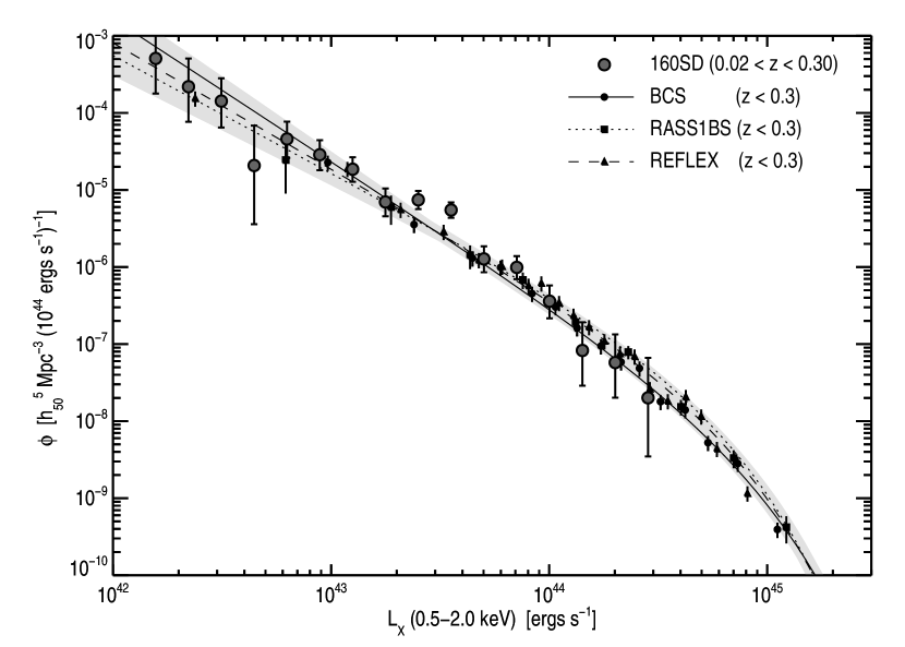
Figure 4.— Determinations of the local cluster X-ray luminosity function as measured by the 160SD survey and the local reference samples (BCS, RASS1BS, and REFLEX) in an Einstein–de-Sitter universe. The 160SD data values along with the number of clusters and average cluster redshift for each luminosity bin are given in Table 3.2. Nonparametric data points and Schechter fits for the reference samples are from Ebeling et al. (1997), De Grandi et al. (1999b), and Böhringer et al. (2002), respectively. The BCS data points are based on a merged analysis of the BCS+eBCS samples (H. Ebeling 2003, private communication). The shaded region indicates the $1\sigma$ uncertainty envelope of the Schechter fits assuming the errors on $L_{\rm X}^{\star}$ and $\alpha$ are correlated. The indicated uncertainties on data points are $\pm 1\sigma$.

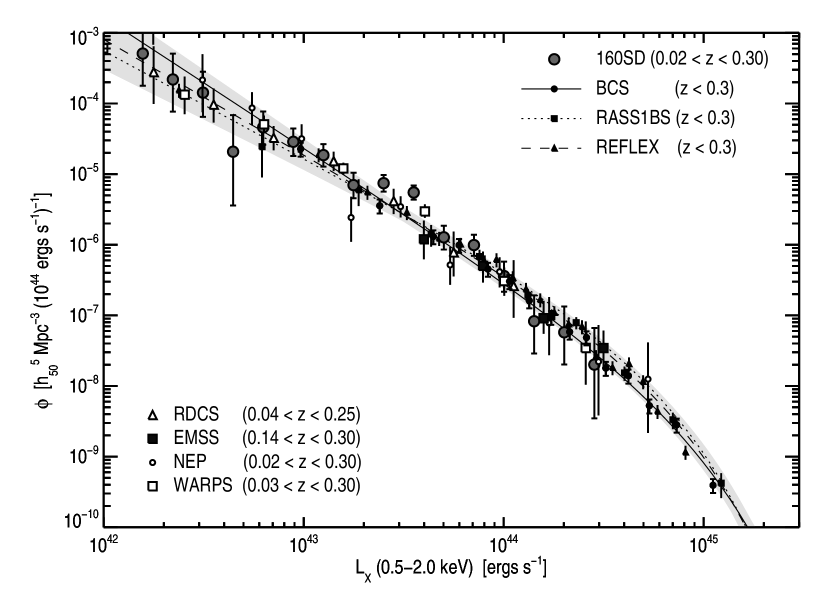
Figure 5.— Compilation of local XLFs as measured by eight X-ray flux-limited surveys. RDCS: Rosati et al. (1998), EMSS: Henry et al. (1992), NEP: Gioia et al. (2001), and WARPS: Jones et al. (2000b) and the references in Figure 4 (Einstein–de-Sitter universe).

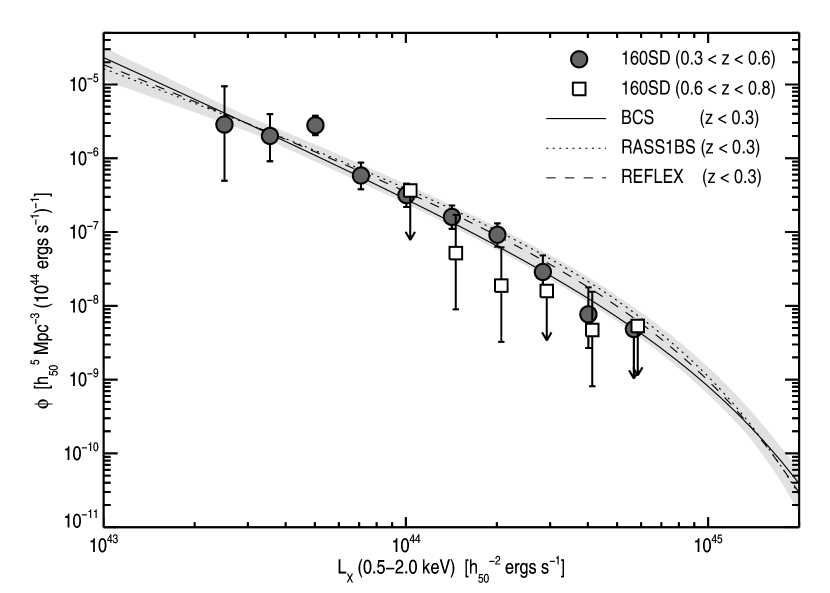
Figure 6.— The high-redshift cluster X-ray luminosity function from the 160SD sample (Einstein–de-Sitter universe). The data points for $0.6<z<0.8$ have been slightly offset to avoid confusion. The 160SD data values along with the number of clusters and average cluster redshift for each luminosity bin are given in Table 3.2. Schechter fits to the local XLF are also plotted as described in Figure 4. If no clusters are detected in a luminosity bin, we plot the $1\sigma$ upper limit for the Poisson error on zero clusters.

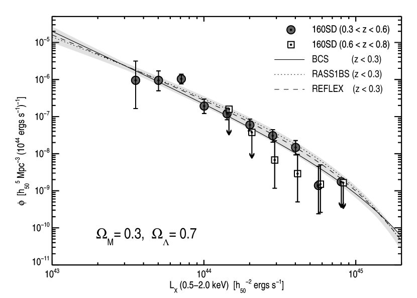
Figure 7.— The high-redshift cluster X-ray luminosity function from the 160SD sample for a cosmology characterized by the parameters $\Omega_{M}=0.3$ and $\Omega_{\Lambda}=0.7$. The data points for $0.6<z<0.8$ have been slightly offset to avoid confusion. The 160SD data values along with the number of clusters and average cluster redshift for each luminosity bin are given in Table 3.2. The REFLEX XLF was explicitly measured for a $\Lambda$-dominated cosmology by Böhringer et al. (2002). We transform the BCS and RASS1BS results to this cosmology based on the REFLEX results (see text for details).

Table 2Local 160SD Cluster X-ray Luminosity Function ($0.02<z<0.3$, EdS)

$L_{\rm X}$(center)	$L_{\rm X}$(min)	$L_{\rm X}$(max)	$\phi(L_{\rm X})$	$\phi(L_{\rm X})_{-1\sigma}$	$\phi(L_{\rm X})_{+1\sigma}$	$<z>$	$N_{\rm cl}$
($10^{44}$ $h_{50}^{-2}$ ergs s-1)	$\cdots$	$\cdots$	($h_{50}^{5}$ Mpc-3 (1044 ergs s-1)-1)	$\cdots$	$\cdots$
0.016	0.013	0.019	5.09 $\times$ 10-4	1.78 $\times$ 10-4	1.18 $\times$ 10-3	0.045	2
0.022	0.019	0.026	2.19 $\times$ 10-4	7.65 $\times$ 10-5	5.07 $\times$ 10-4	0.035	2
0.031	0.026	0.037	1.42 $\times$ 10-4	6.45 $\times$ 10-5	2.81 $\times$ 10-4	0.062	3
0.044	0.037	0.053	2.08 $\times$ 10-5	3.59 $\times$ 10-6	6.85 $\times$ 10-5	0.135	1
0.063	0.053	0.075	4.59 $\times$ 10-5	2.61 $\times$ 10-5	7.69 $\times$ 10-5	0.142	5
0.089	0.075	0.106	2.87 $\times$ 10-5	1.80 $\times$ 10-5	4.42 $\times$ 10-5	0.136	7
0.125	0.106	0.149	1.86 $\times$ 10-5	1.28 $\times$ 10-5	2.65 $\times$ 10-5	0.156	10
0.177	0.149	0.211	6.98 $\times$ 10-6	4.55 $\times$ 10-6	1.04 $\times$ 10-5	0.154	8
0.251	0.211	0.298	7.44 $\times$ 10-6	5.65 $\times$ 10-6	9.72 $\times$ 10-6	0.200	17
0.355	0.298	0.422	5.49 $\times$ 10-6	4.35 $\times$ 10-6	6.89 $\times$ 10-6	0.197	23
0.502	0.422	0.597	1.27 $\times$ 10-6	8.55 $\times$ 10-7	1.86 $\times$ 10-6	0.195	9
0.710	0.597	0.844	9.89 $\times$ 10-7	6.94 $\times$ 10-7	1.39 $\times$ 10-6	0.239	11
1.004	0.844	1.194	3.60 $\times$ 10-7	2.16 $\times$ 10-7	5.76 $\times$ 10-7	0.226	6
1.420	1.194	1.688	8.26 $\times$ 10-8	2.89 $\times$ 10-8	1.92 $\times$ 10-7	0.225	2
2.008	1.688	2.388	5.76 $\times$ 10-8	2.01 $\times$ 10-8	1.34 $\times$ 10-7	0.180	2
2.840	2.388	3.377	2.01 $\times$ 10-8	3.47 $\times$ 10-9	6.63 $\times$ 10-8	0.296	1

Our measurement of the XLF at $0.3<z<0.6$ probes the luminosity range 2 $\times$ 10⁴³ – 7 $\times$ 10⁴⁴ ergs s^-1  (Figure 6: filled circles). Except for the data point near 5 $\times$ 10⁴³ ergs s^-1 which is $1.9\sigma$ off the local relation, there is excellent agreement between these results and the no-evolution benchmark at least out to intermediate luminosities, $L_{\rm X}\sim$ 2 $\times$ 10⁴⁴ ergs s^-1. In this region the 160SD best matches the normalization of the REFLEX XLF. At higher luminosities the distant XLF is lower than the local population but we will demonstrate in § 4.1 that this effect is only marginally significant with respect to the local XLF with the highest normalization (RASS1BS). The median redshift for these depressed data points is $<z>=0.50$ (see Table 3.2).

At the highest redshifts probed by the 160SD in the present analysis, $0.6<z<0.8$, we measure useful constraints over the luminosity interval 1 – 6 $\times$ 10⁴⁴ ergs s^-1, and the median cluster redshift is $<z>=0.70$. (Figure 6: open squares). The distant cluster volume densities are below the local level at all measured luminosities. We will show that this result is significant ($>3\sigma$) in both the Einstein–de-Sitter and $\Lambda$-dominated models even with respect to the lowest-normalization local XLF (§ 4.1). This is a deficit of high luminosity, high redshift clusters in a manner similar to that seen in the EMSS results. Note that although the optical CCD imaging used to identify the 160SD clusters was sufficiently deep to reveal massive clusters to $z=0.9$, we have conservatively cut off the most distant redshift shell at $z=0.8$. This lessens any potential negative evolution in the results since the larger redshift boundary would increase the search volume without adding clusters and hence depress the data points.

To assess the impact of changing the cosmological framework from an Einstein–de-Sitter to a $\Lambda$-dominated universe, we repeat our calculation of the cluster luminosity function setting $\Omega_{M}=0.3$ and $\Omega_{\Lambda}=0.7$, the results of which are shown in Figure 7 and Table 3.2. The Einstein–de-Sitter XLF ($\phi_{\rm EdS}$, Figure 6) and $\Lambda$-dominated XLF ($\phi_{\Lambda}$) appear very similar because the data points of the latter are offset diagonally down and to the right approximately along the former. This is the combined effect of the increase in both the cluster luminosities and the search volumes in a $\Lambda$-dominated universe. The actual positioning of the two XLFs relative to each other depends on the cluster redshifts and the specific luminosity interval. For example in the REFLEX survey ($<z>=0.08$), between 10⁴³ and 10⁴⁵ ergs s^-1  the ratio of the fitted XLFs ($\phi_{\Lambda}$/$\phi_{\rm EdS}$) is less than unity with a broad minimum of $\sim$0.8 around 10⁴⁴ ergs s^-1. REFLEX is the only local sample for which the XLF in a $\Lambda$-cosmology has been explicitly measured (Böhringer et al., 2002). However, given the similarity of the redshift and luminosity distributions, we have used the ratio $\phi_{\Lambda}$/$\phi_{\rm EdS}$ from REFLEX to make an approximate transform of the BCS and RASS1BS to this alternate cosmology.

It is apparent from Figure 7 that the high-redshift 160SD XLFs and the local XLFs shift in similar ways; thus the apparent deficit of high-luminosity clusters persists in the $\Lambda$-dominated cosmology. The only important difference, of course, is that the point where the 160SD data depart significantly from the non-evolution baseline is shifted to larger luminosities, and this is anticipated given the increase in luminosity distance ($L_{\rm X}\gtrsim$ 3 $\times$ 10⁴⁴ ergs s^-1  for $0.3<z<0.6$, and $L_{\rm X}\gtrsim$ 2 $\times$ 10⁴⁴ ergs s^-1  for $0.6<z<0.8$).

We will examine the significance and strength of this apparent cluster evolution in the following section.

Table 3Distant 160SD Cluster X-ray Luminosity Function (EdS)

$0.6<z<0.8$    1.004 0.844 1.194 3.65 $\times$ 10^-7 $\cdots$ 3.65 $\times$ 10^-7 $\cdots$ 0 1.420 1.194 1.688 5.17 $\times$ 10^-8 8.95 $\times$ 10^-9 1.71 $\times$ 10^-7 0.699 1 2.008 1.688 2.388 1.88 $\times$ 10^-8 3.25 $\times$ 10^-9 6.20 $\times$ 10^-8 0.625 1 2.840 2.388 3.377 1.59 $\times$ 10^-8 $\cdots$ 1.59 $\times$ 10^-8 $\cdots$ 0 4.016 3.377 4.776 4.71 $\times$ 10^-9 8.15 $\times$ 10^-10 1.55 $\times$ 10^-8 0.700 1 5.679 4.776 6.754 5.33 $\times$ 10^-9 $\cdots$ 5.33 $\times$ 10^-9 $\cdots$ 0

Table 4Distant 160SD Cluster X-ray Luminosity Function ($\Omega_{M}=0.3$ and $\Omega_{\Lambda}=0.7$)

$0.6<z<0.8$    1.420 1.194 1.688 1.59 $\times$ 10^-7 $\cdots$ 1.59 $\times$ 10^-7 $\cdots$ 0 2.008 1.688 2.388 3.75 $\times$ 10^-8 $\cdots$ 3.75 $\times$ 10^-8 $\cdots$ 0 2.840 2.388 3.377 6.76 $\times$ 10^-9 1.17 $\times$ 10^-9 2.23 $\times$ 10^-8 0.699 1 4.016 3.377 4.776 2.90 $\times$ 10^-9 5.02 $\times$ 10^-10 9.57 $\times$ 10^-9 0.625 1 5.679 4.776 6.754 1.51 $\times$ 10^-9 2.61 $\times$ 10^-10 4.98 $\times$ 10^-9 0.700 1 8.032 6.754 9.552 1.65 $\times$ 10^-9 $\cdots$ 1.65 $\times$ 10^-9 $\cdots$ 0

4. Quantifying Evolution

X-ray luminosity functions like those shown in Figures 4–7 are useful for visualizations and qualitative assessments of the cluster population; however, they are non-optimal for quantitative analyses. For example ambiguities exist in the selection of the luminosity binning (e.g., fixed or adaptive intervals) and the loci of the plotted data points in luminosity space (e.g., at the bin center or the density-weighted mean luminosity). Furthermore, for the case of negative evolution the effect that we are attempting to measure is either a diminishing signal or a non-detection. Thus we will apply the alternate approaches of integrated number counts and a maximum-likelihood fit of an evolving model XLF to quantify the significance and strength of the apparent evolution in the 160SD clusters.

Table 5Observed versus Expected Number of Clusters ($L_{\rm X,min}<L_{\rm X}<\infty$)

$0.3<z<0.6$, $\Omega_{M}=0.3$ and $\Omega_{\Lambda}=0.7$    6.75400003.503.004.001.91.62.1 4.77601007.806.109.102.72.23.1 3.37708014.811.017.401.70.72.3 2.38817024.417.828.801.40.02.2   $0.6<z<0.8$, EdS    4.77600004.103.204.802.11.72.4 3.37701007.905.809.302.72.03.1 2.38801012.609.114.903.93.14.4 1.68802017.212.520.204.43.45.0 1.19403020.515.024.104.63.55.2 0.84403022.016.125.704.93.85.5   $0.6<z<0.8$, $\Omega_{M}=0.3$ and $\Omega_{\Lambda}=0.7$    6.75400003.803.304.402.01.82.2 4.77601007.806.109.002.72.23.0 3.37702012.709.614.903.42.73.9 2.38803017.412.920.504.03.14.6 1.68803020.615.224.204.63.65.2 1.19403021.816.125.604.83.85.5

4.1. Integrated Number Counts

For a given region of luminosity-redshift space we compare the number of observed clusters ($N_{\rm obs}$) with the number that are expected ($N_{\rm exp}$) assuming there is no evolution in the population. The latter is computed by integrating the local luminosity function, $\phi(L_{\rm X},z$), over luminosity and redshift, and folding this through the survey selection function, $\Omega(f_{\rm X}$), using the following equation,

$$N_{\rm exp}~{}=~{}\int_{L_{\rm X,min}}^{L_{\rm X,max}}\int_{z_{\rm min}}^{z_{\rm max}}\phi(L_{\rm X},z)~{}\Omega(f_{\rm X}(L_{\rm X},z))~{}\frac{dV(z)}{dz}~{}dz~{}dL_{\rm X}.$$ (7)

Note that the non-evolving XLF is strictly a function of luminosity as parameterized by the Schechter fits to local clusters (e.g., Equation 5 with the best-fit parameters from Table 1). However, we explicitly indicate the potential redshift dependence in this equation to generalize it for subsequent treatment with an evolving XLF. The statistical significance of the difference between $N_{\rm obs}$ and $N_{\rm exp}$ is computed based on Poisson confidence intervals (Gehrels, 1986).

Of the three local XLFs (BCS, RASS1BS, and REFLEX), we use the REFLEX measure as the preferred reference for three reasons: 1) the REFLEX local XLF is based on the largest sample of clusters used to date (452 clusters), 2) the REFLEX normalization lies intermediate to the BCS and RASS1BS, and 3) at low to intermediate luminosities, our 160SD low-redshift data most closely match the REFLEX normalization. Nonetheless, we will also quote our results relative to the BCS and RASS1BS to demonstrate the full range of possible significances.

First we consider the redshift interval $0.3<z<0.6$ starting with the highest luminosity bin and then integrating to lower luminosities in an Einstein–de-Sitter model. In and above the highest bin of the XLF ($L_{\rm X}\gtrsim 4.8$), we observe zero clusters whereas the REFLEX local XLF predicts 4.5 clusters according to Equation 7. This difference is only 2.3$\sigma$ significant. The next two bins ($L_{\rm X}\gtrsim 3.4,2.4$) have $N_{\rm obs}=2,7$ and $N_{\rm exp}=9.1,16.2$ with the associated significances of 2.6$\sigma$ and 2.4$\sigma$. Continuing from here to lower luminosity bins decreases the significance. These results are summarized in Table 4. Examining the run of significance versus minimum luminosity without the constraints of the arbitrary bins of Figure 6 indicates that the significance briefly peaks above 3$\sigma$ near 3.4 $\times$ 10⁴⁴ ergs s^-1. However with the BCS XLF as the no-evolution reference, the apparent cluster deficit is not significant (i.e. always $<3\sigma$). Conversely, the RASS1BS XLF indicates a statistically strong signal across much of the probed luminosity. Repeating this analysis in the context of a $\Lambda$-dominated universe uniformly reduces the significance of the cluster deficit such that only relative to the RASS1BS does the deviation seen in the 160SD measure at $0.3<z<0.6$ appear marginally significant (see Table 4).

Our highest redshift measure of the XLF, $0.6<z<0.8$, is clearly lower than all the determinations of the local XLF (Figures 6 & 7). Integrating over the entire luminosity range sampled in this redshift shell, a non-evolving model of the cluster population based on the REFLEX XLF predicts 22.1 clusters. This strongly conflicts with the actual observed sample of 3 clusters, a 4.9$\sigma$ difference. The situation in the $\Lambda$-cosmology is essentially the same; 21.8 clusters expected, a 4.8$\sigma$ difference. If we instead use the RASS1BS XLF as our baseline, the predicted count is greater than 26 clusters with the resulting cluster deficit being 5.5$\sigma$. More importantly, if we adopt the most conservative position (i.e., attempting to minimize the deficit) and use the BCS XLF, we expect to find 16 clusters which is 3.8$\sigma$ away from the observed value. An integrated bin-by-bin analysis is reported in Table 4.

4.2. Maximum Likelihood Analysis

A more general approach to quantifying evolution in the cluster XLF is to perform a maximum likelihood fit of an evolving Schechter function to the observed cluster distribution in luminosity and redshift. This approach makes maximal use of the data, is free from arbitrary binning, and is sensitive to potential negative evolution (Rosati et al., 2000; Henry, 2002).

We follow the prescription of Marshall et al. (1983) but generalize the treatment to account for uncertainties in the observations. The luminosity-redshift plane is uniformly parsed into extremely small intervals of size $dL_{\rm X}dz$. In each element we compute the expected number of clusters with luminosity $L_{\rm X}$ and redshift $z$:

$$\lambda(L_{\rm X},z)dL_{\rm X}dz~{}=~{}\phi(L_{\rm X},z)~{}\Omega(f_{\rm X}(L_{\rm X},z))~{}\frac{dV(z)}{dz}dL_{\rm X}dz.$$ (8)

The model XLF, $\phi(L_{\rm X},z)$, is an evolving Schechter function of the form given in Equation 5. The important modification here is to free the density normalization, $\phi^{\star}$, and characteristic luminosity, $L_{\rm X}^{\star}$, of the luminosity function to evolve with redshift such that,

$$\phi^{\star}(z)~{}=\phi^{\star}_{0}~{}\left(\frac{1+z}{1+z_{0}}\right)^{A},$$ (9)

and

$$L_{\rm X}^{\star}(z)~{}=L_{{\rm X},0}^{\star}\left(\frac{1+z}{1+z_{0}}\right)^{B},$$ (10)

where $A$ and $B$ parameterize the evolution. The local values of the normalization ($\phi^{\star}_{0}$) and characteristic luminosity ($L^{\star}_{{\rm X},0}$) are taken from the local XLF determination which samples a median redshift of $z_{0}$. This redshift baseline is luminosity dependent as a result of the flux-limited nature of the survey technique. For instance in the BCS sample, at $L_{\rm X}$ = 0.1 (1, 10) $\times$ 10⁴⁴ ergs s^-1, the median sample redshift is $z_{0}=0.02$ (0.06, 0.21). Note that in the present model the faint-end slope of the luminosity function ($\alpha$) is fixed at the local value since there is little evidence for any change in this parameter as a function of redshift.

The sampling of the luminosity-redshift plane is sufficiently fine that in each element, $dL_{\rm X}dz$, the number of observed clusters is either zero or one and the expected number of clusters is much smaller than unity. In this sparse sampling limit we can define a likelihood function $\cal{L}$ based on joint Poisson probabilities,

$${\cal{L}}~{}=~{}\prod_{i}\lambda(L_{{\rm X},i},z_{i})dL_{{\rm X}}dz~{}e^{-\lambda(L_{{\rm X},i},z_{i})dL_{{\rm X}}dz}$$

$$\times~{}\prod_{j}e^{-\lambda(L_{{\rm X},j},z_{j})dL_{{\rm X}}dz.}$$ (11)

This is the combined probability of observing exactly one cluster at each point ($L_{{\rm X},i},z_{i}$) populated by a 160SD cluster and observing exactly zero clusters everywhere else ($L_{{\rm X},j},z_{j}$). Again, occupied elements in the luminosity-redshift plane are indexed by $i$, whereas empty elements are indexed by $j$. Transforming to the standard expression, $S=-2\ln{\cal{L}}$, and dropping terms that are not model dependent, we have

$$S=-2\sum_{i}w_{i}~{}\ln[\lambda(L_{{\rm X},i},z_{i})]~{}$$

$$+~{}2\int_{L_{\rm X,min}}^{L_{\rm X,max}}\int_{z_{\rm min}}^{z_{\rm max}}\lambda(L_{{\rm X}},z)dL_{{\rm X}}dz.$$ (12)

A weighting term, $w_{i}$, is introduced to incorporate the uncertainties in observed cluster luminosity and the summation is evaluated over a total number of $i$ indices much greater than the number of observed clusters (e.g., Borgani et al., 2001). Instead of being a point in the observed ($L_{\rm X},z$)-plane, each cluster is smoothed in the $L_{\rm X}$-direction according to a Gaussian distribution with a width set by the 1$\sigma$ flux error, $\epsilon_{L_{\rm X}}$, for each cluster (median value is 20% for the 160SD sample). No similar treatment is required for the redshift measures since the typical error is a few tenths of a percent. Thus a weight is assigned to each element in the luminosity-redshift plane based on the fractional contributions of all clusters in the same redshift interval,

$$w_{i}~{}=~{}\sum_{k}\frac{1}{\sqrt{2\pi\epsilon_{L_{{\rm X},k}}^{2}}}~{}\exp{\left[-\frac{(L_{{\rm X},k}-L_{{\rm X},i})^{2}}{2\epsilon_{L_{{\rm X},k}}^{2}}\right]}dL_{\rm X}.$$ (13)

Here the summation $k$ is over the clusters with a redshift between $z_{i}-dz/2$ and $z_{i}+dz/2$.

Recall the overall goal is to find the values of $A$ and $B$ that predict a luminosity-redshift distribution that best matches the data. These best-fit parameters are determined by minimizing $S$ with confidence levels defined to be

$$\Delta S~{}=~{}S(A,B)-S(A_{\rm best},B_{\rm best})$$ (14)

Since $S$ is distributed like $\chi^{2}$, the $1\sigma$, $2\sigma$, and $3\sigma$ (68.3%, 95.4%, and 99.7%) confidence intervals for a two parameter fit are $\Delta S=2.30$, 6.17, and 11.8, respectively (Avni, 1976; Cash, 1976, 1979).

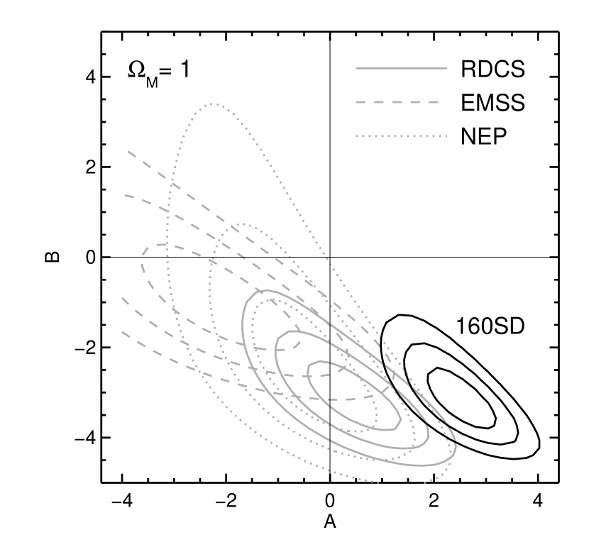
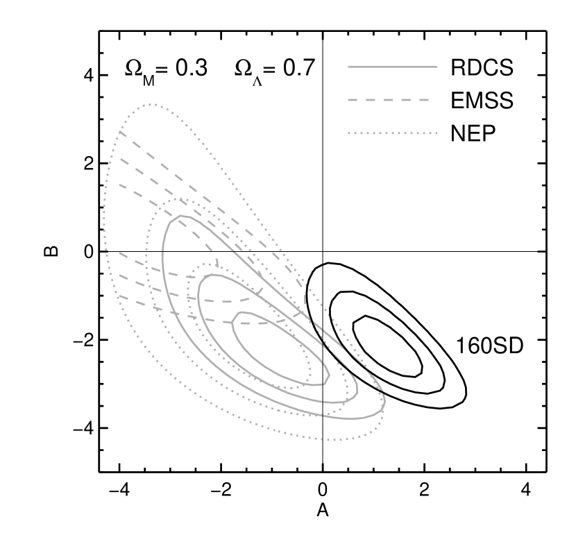
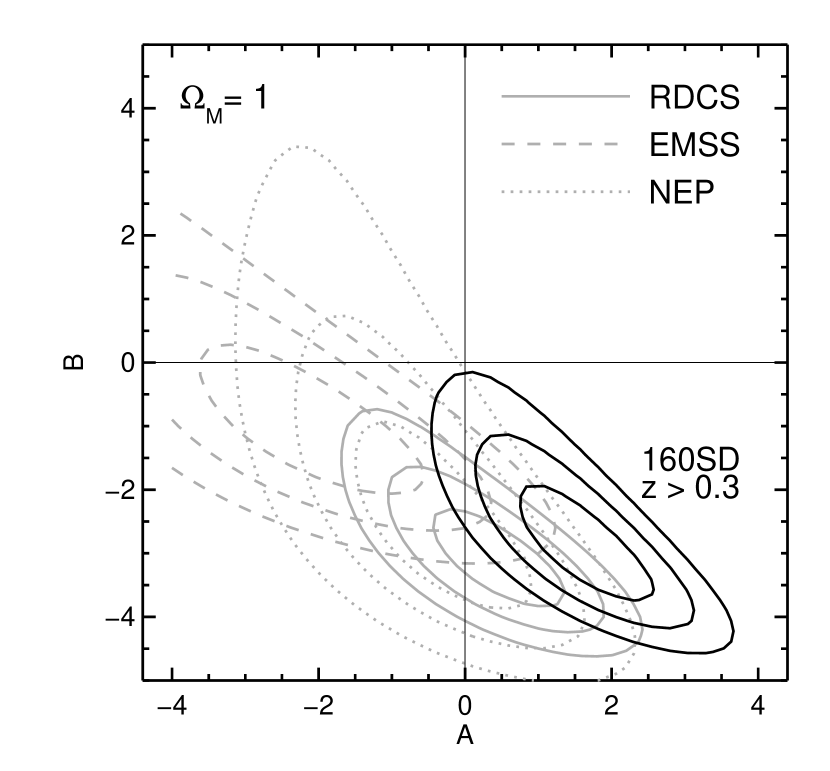
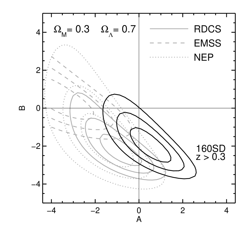
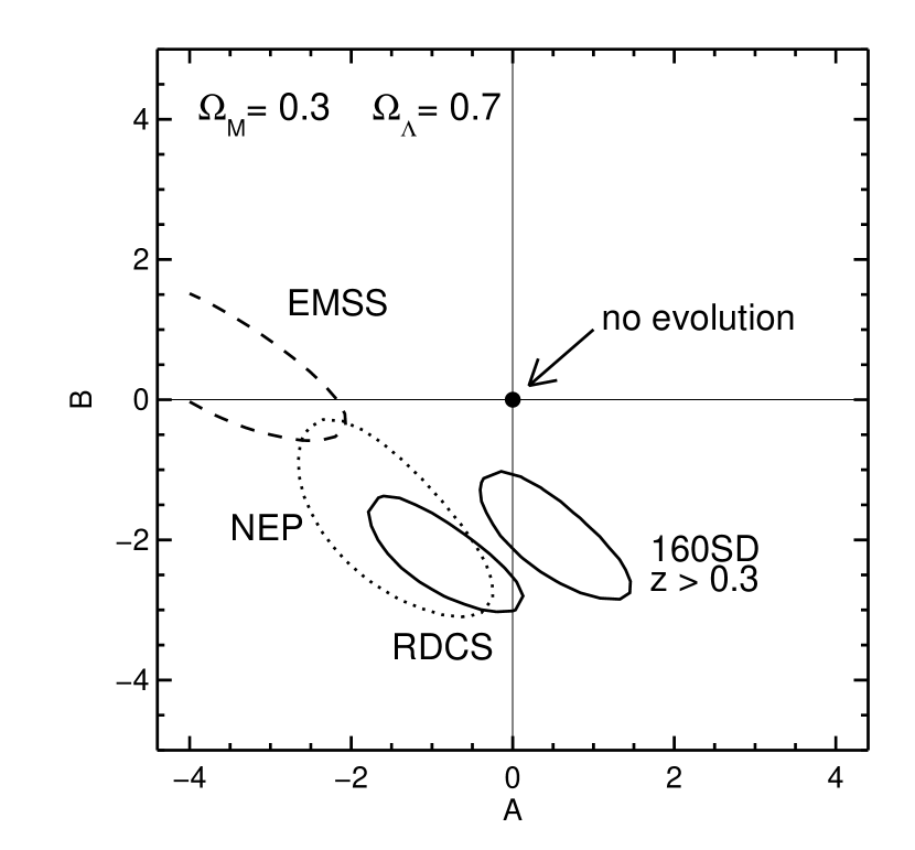
Figure 8.— Maximum-likelihood contours for the parameters A and B characterizing the evolution of the cluster XLF where $\phi^{\star}\propto\phi^{\star}_{0}(1+z)^{A}$ and $L_{\rm X}^{\star}\propto L_{{\rm X},0}^{\star}(1+z)^{B}$ based on four independent surveys. Plotted are the results from our analysis of the 160SD and NEP samples, plus similar data for the EMSS and RDCS from Rosati et al. (2002). The no-evolution scenario corresponds to $A=B=0$. Confidence regions in the left column are computed in an Einstein–de-Sitter universe, whereas those in the right column are for a $\Lambda$-dominated universe. TOP PANELS: One, two, and three $\sigma$ contours with the 160SD results based on the entire sample. MIDDLE PANELS: One, two, and three $\sigma$ contours with the 160SD results based on the $z>0.3$ sample. BOTTOM PANELS: Same as the middle panels except only $1\sigma$ contours are shown for clarity.

We use the maximum-likelihood procedure to estimate the evolutionary parameters for a model XLF that best reproduces the observed cluster luminosity-redshift distribution. For the local parameters of the XLF ($\phi^{\star}_{0}$, $L_{{\rm X},0}$, and $\alpha$) we adopt the values from the BCS. This permits comparisons to previous work and assumes a conservative position since the BCS has the lowest normalization of the three local references. We estimated the baseline redshift, $z_{0}(L_{\rm X}$), by calculating the median redshifts in seven luminosity intervals of the BCS sample and interpolating across these points ($z_{0}$ = 0.018, 0.028, 0.040, 0.061, 0.103, 0.171, 0.236 at $L_{\rm X,EdS}$/10⁴⁴ = 0.054, 0.139, 0.303, 0.938, 2.283, 5.771, 12.929 ergs s^-1). The top panels of Figure 8 indicate the constraints using the entire 160SD sample of 177 clusters ($0.02<z<0.80$, 10${}^{42}<L_{\rm X}<10^{46}$, $f_{\rm X}>4\times 10^{-14}$) in two different cosmologies: $A=2.6^{+0.6}_{-0.7}$, $B=-3.2^{+0.8}_{-0.6}$ (EdS), $A=1.3^{+0.6}_{-0.7}$, $B=-2.3^{+0.8}_{-0.6}$ ($\Lambda$-cosmo). In either case, no evolution ($A=B=0$) is strongly excluded at $>3\sigma$.

To examine the evolution “signal” in the 160SD sample at higher redshifts corresponding to the XLFs in Figures 6 & 7, we repeat the maximum-likelihood analysis using the 66 clusters at $z>0.3$. The resulting contours are shown in the middle panels of Figure 8 and the best-fit values are: $A=1.6^{+1.0}_{-0.8}$, $B=-2.9^{+1.0}_{-0.8}$ (EdS), $A=0.6^{+0.9}_{-1.0}$, $B=-2.1^{+1.0}_{-0.8}$ ($\Lambda$-cosmo). Relative to the full sample analysis, the best-fit $A$ is about $1\sigma$ lower while the best-fit $B$ is effectively unchanged, being a few tenths of $\sigma$ lower. Apparently, the $A\/$ parameter in the full analysis is elevated to fit an enhancement of clusters at $z<0.3$ which can be seen at $\sim 3\times$ 10⁴³ ergs s^-1 in the low-redshift XLF. We adopt the less-biased $z>0.3$ results as representative of the 160SD in subsequent discussions.

For comparison purposes, we also show in Figure 8 the constraints from three additional datasets — the NEP, EMSS, and RDCS. One, two and three $\sigma$ contours are shown in the top and middle panels, whereas only $1\sigma$ contours are plotted in bottom panels. The degree of agreement amongst the four surveys is reasonably good but certainly not perfect. It is not immediately clear how much of this is due to potential systematics in the individual datasets or the appropriateness of the model XLF used in the maximum-likelihood fit. These issues will be addressed in a forthcoming paper focused on the joint analysis of the available samples (J. P. Henry et al. 2004, in preparation; preliminary results discussed in Henry, 2003).

Considering the ensemble of data from four independent cluster samples, the no-evolution scenario ($A=B=0$) is strongly ruled out at $\gg 3\sigma$ at $z\lesssim 0.8$ regardless of cosmology. In an Einstein–de-Sitter universe, the change in the cluster population is consistent with pure luminosity evolution ($A\approx 0,B\approx-2.5$), whereas it may be a combination of luminosity and density evolution ($A\approx-1,B\approx-2$) in a $\Lambda$-dominated universe. Given the lack of clusters with $L_{\rm X}>10^{45}$ ergs s^-1 in the analyzed samples, caution is warranted if these results are extrapolated to predict the cluster abundance at very high luminosities. Nonetheless, we show in Figure 9 that our characterization of cluster evolution is consistent with a direct measurement of the comoving volume density of clusters at $L_{\rm X}>10^{45}$ from the eBCS+MACS surveys (H. Ebeling et al. 2004, in preparation).

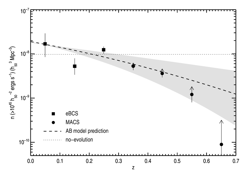
Figure 9.— Comoving volume density of very X-ray luminous clusters with $L_{\rm X}>10^{45}$ ergs s^-1  (0.1–2.4 keV; equivalently $>$6.2 $\times$ 10⁴⁴, 0.5–2.0 keV). The data points are derived from the eBCS and the MACS samples as reported by H. Ebeling et al. (see Figure 5 in Ellis, 2002, and H. Ebeling et al. 2004, in preparation) in an Einstein–de-Sitter universe. The dashed line and shaded region indicate the prediction based on our ensemble best-fit model XLF ($A=0,B=-2.5\pm 1$); not a fit to the eBCS+MACS data. The dotted line marks the no-evolution expectation derived from the BCS Schechter function fit to the local XLF which is dominated by $z\sim 0.2$ clusters at these luminosities.

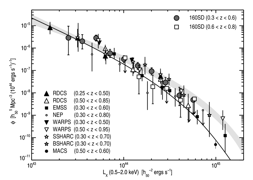
Figure 10.— Compilation of high-redshift XLFs as measured by eight independent X-ray flux-limited surveys (Einstein–de-Sitter universe). References are 160SD (this paper), RDCS (Rosati et al., 2000), EMSS (Henry et al., 1992), NEP (Gioia et al., 2001), WARPS (Jones et al., 2000b), SSHARC (Burke et al., 1997), BSHARC (Nichol et al., 1999), and MACS (H. Ebeling 2003, private communication). The shaded region delineates the regime of the local XLF whereas the heavy solid line is an evolving model XLF ($A=0$, $B=-2.5$) at $z=0.7$.

5. Conclusions

We have used the 160SD sample of 201 X-ray selected galaxy clusters to track the volume density of these systems at local, intermediate and high redshifts. Nonparametric measurements of the cluster XLF suggest there is effectively no detectable evolution in the population out to $z\sim 0.6$ at luminosities less than a few times 10⁴⁴ $h_{50}^{-2}$ ergs s^-1. However, data in the redshift interval $0.6<z<0.8$ indicate a mild but significant ($>3\sigma$) change in volume densities above luminosities of approximately 10⁴⁴ $h_{50}^{-2}$ ergs s^-1. Our findings demonstrate a deficit of high-luminosity clusters at high redshift relative to the present-day levels. For example, we observe only 3 clusters at $0.6<z<0.8$ where an integral over the local XLF predicts we should find at the very least 16 clusters. A maximum-likelihood analysis of the observed luminosity-redshift distribution further underscores that the no-evolution scenario is entirely inconsistent with 160SD data. Modelling the XLF with an evolving Schechter function, we have demonstrated that the 160SD, NEP, RDCS and EMSS clusters samples all reject a model lacking evolution. Further our evolving XLF model derived from datasets at $L_{\rm X}<10^{45}$ successfully predicts the observed volume densities at $L_{\rm X}>10^{45}$.

A composite view of the high-redshift cluster population is shown in Figure 10. Here we plot the latest compilation of distant XLFs as measured by eight X-ray flux-limited surveys. From these data six independent teams have concluded there is measurable cluster evolution — EMSS: Gioia et al. (1990a); Henry et al. (1992), BSHARC: Nichol et al. (1999), RDCS: Rosati et al. (2000), NEP: Gioia et al. (2001), 160SD: this work, and MACS (H. Ebeling 2004, in preparation). Conversely, SSHARC (Burke et al., 1997) and WARPS (Jones et al., 2000a) draw the opposite conclusion. Note however that the sky coverage of the SSHARC survey (17.7 deg²) is inadequate to measure evolutionary changes at the very bright end of the XLF, as studied in the large solid angle EMSS (735 deg²) and the 160SD surveys.

Measurements of the cluster X-ray luminosity function are consistent with a population whose comoving volume density evolves as a function of both redshift and luminosity (mass). For a sample of distant clusters in a fixed luminosity interval, the difference in volume density for this sample relative to the present-day population increases with increasing redshift (e.g., Figure 9). Considering a sample of clusters in a distant redshift interval, the difference in volume density for this sample and the present-day population increases with increasing luminosity (e.g., Figure 10). Visualizing this on the luminosity-redshift plane, the cluster deficit is maximal at high redshift and high luminosity (i.e., the upper-right corner of Figure 1). The maximum-likelihood results in Figure 8 demonstrate that the EMSS, 160SD, RDCS, and NEP surveys all reject the no-evolution scenario and generally agree on the character of the evolution (e.g., AB contours overlap at 1–2 $\sigma$). The EMSS was able to detect a statistically significant cluster deficit in the $0.3<z<0.6$ redshift shell because of their sensitivity to very luminous clusters. Surveys such as the 160SD probe lower luminosities where the evolution “signal” is intrinsically weaker and thus have to push to higher redshifts (e.g., $0.6<z<0.8$) before the deficit grows large enough for a significant detection.

The preponderance of observational data requires mild evolution in the bright end of the cluster XLF as measured out to $z\sim 0.8$, whereas the volume densities of the bulk of the population (low and intermediately massive systems) do not change appreciably. In the context of hierarchical structure formation, we are probing sufficiently large mass aggregations at sufficiently early times where the Universe has yet to assemble these clusters to present-day volume densities. Cosmological constraints derived from the RDCS and 160SD samples (Borgani et al., 2001; Vikhlinin et al., 2003) demonstrate the observed evolution is consistent with structure growth in a flat universe with $\Omega_{\rm M}\sim 0.3$.

A decade after the first evidence for negative cluster evolution reported by the Einstein EMSS survey (Gioia et al., 1990a; Henry et al., 1992), we are now witnessing the fruition of the ROSAT era cluster surveys: 1) the robust determination of the local cluster X-ray luminosity function, and 2) multiple, independent confirmations of the EMSS results on cluster evolution. Further work remains to assimilate the available cluster samples in a detailed, joint analysis to produce maximal constraints on the evolution phenomenon. Furthermore, additional inputs are expected in the near term from two on-going surveys — BMW-HRI (Panzera et al., 2003) and MACS (Ebeling et al., 2001). The BMW-HRI has a sky coverage rather similar to the 160SD, and hence will likely provide similar XLF measures. The final results from MACS should prove particularly interesting because this program probes extremely high luminosities ($L_{\rm X}\gtrsim 10^{45}$ ergs s^-1) at high redshift exactly where the evolution signature should be strongest. Finally, on longer timescales, searches with XMM-Newton and possibly a new dedicated X-ray survey satellite should reveal substantial numbers of $z>1$ clusters which will provide powerful leverage in the study of cluster evolution.

References

- Avni (1976) Avni, Y. 1976, ApJ, 210, 642
- Avni & Bahcall (1980) Avni, Y. & Bahcall, J. N. 1980, ApJ, 235, 694
- Bahcall et al. (1999) Bahcall, N. A., Ostriker, J. P., Perlmutter, S., & Steinhardt, P. J. 1999, Science, 284, 1481
- Böhringer et al. (2002) Böhringer, H., Collins, C. A., Guzzo, L., Schuecker, P., Voges, W., Neumann, D. M., Schindler, S., Chincarini, G., De Grandi, S., Cruddace, R. G., Edge, A. C., Reiprich, T. H., & Shaver, P. 2002, ApJ, 566, 93
- Böhringer et al. (2001) Böhringer, H., Schuecker, P., Guzzo, L., Collins, C. A., Voges, W., Schindler, S., Neumann, D. M., Cruddace, R. G., De Grandi, S., Chincarini, G., Edge, A. C., MacGillivray, H. T., & Shaver, P. 2001, A&A, 369, 826
- Borgani & Guzzo (2001) Borgani, S. & Guzzo, L. 2001, Nature, 409, 39
- Borgani et al. (2001) Borgani, S., Rosati, P., Tozzi, P., Stanford, S. A., Eisenhardt, P. R., Lidman, C., Holden, B., Della Ceca, R., Norman, C., & Squires, G. 2001, ApJ, 561, 13
- Burke et al. (1997) Burke, D. J., Collins, C. A., Sharples, R. M., Romer, A. K., Holden, B. P., & Nichol, R. C. 1997, ApJ, 488, L83
- Burke et al. (2003) Burke, D. J., Collins, C. A., Sharples, R. M., Romer, A. K., & Nichol, R. C. 2003, MNRAS, 341, 1093
- Cash (1976) Cash, W. 1976, A&A, 52, 307
- Cash (1979) —. 1979, ApJ, 228, 939
- Castander et al. (1995) Castander, F. J., Bower, R. G., Ellis, R. S., Aragon-Salamanca, A., Mason, K. O., Hasinger, G., McMahon, R. G., Carrera, F. J., Mittaz, J. P. D., Perez-Fournon, I., & Lehto, H. J. 1995, Nature, 377, 39
- De Grandi et al. (1999a) De Grandi, S., Böhringer, H., Guzzo, L., Molendi, S., Chincarini, G., Collins, C., Cruddace, R., Neumann, D., Schindler, S., Schuecker, P., & Voges, W. 1999a, ApJ, 514, 148
- De Grandi et al. (1999b) De Grandi, S., Guzzo, L., Böhringer, H., Molendi, S., Chincarini, G., Collins, C., Cruddace, R., Neumann, D., Schindler, S., Schuecker, P., & Voges, W. 1999b, ApJ, 513, L17
- Ebeling et al. (2000a) Ebeling, H., Edge, A. C., Allen, S. W., Crawford, C. S., Fabian, A. C., & Huchra, J. P. 2000a, MNRAS, 318, 333
- Ebeling et al. (1998) Ebeling, H., Edge, A. C., Bohringer, H., Allen, S. W., Crawford, C. S., Fabian, A. C., Voges, W., & Huchra, J. P. 1998, MNRAS, 301, 881
- Ebeling et al. (1997) Ebeling, H., Edge, A. C., Fabian, A. C., Allen, S. W., Crawford, C. S., & Boehringer, H. 1997, ApJ, 479, L101
- Ebeling et al. (2001) Ebeling, H., Edge, A. C., & Henry, J. P. 2001, ApJ, 553, 668
- Ebeling et al. (2000b) Ebeling, H., Jones, L. R., Perlman, E., Scharf, C., Horner, D., Wegner, G., Malkan, M., Fairley, B. W., & Mullis, C. R. 2000b, ApJ, 534, 133
- Ebeling et al. (2002) Ebeling, H., Mullis, C. R., & Tully, R. B. 2002, ApJ, 580, 774
- Edge et al. (1990) Edge, A. C., Stewart, G. C., Fabian, A. C., & Arnaud, K. A. 1990, MNRAS, 245, 559
- Eke et al. (1998) Eke, V. R., Cole, S., Frenk, C. S., & Henry, J. P. 1998, MNRAS, 298, 1145
- Ellis (2002) Ellis, R. S. 2002, in ASP Conf. Ser. 268: Tracing Cosmic Evolution with Galaxy Clusters, 311
- Ellis & Jones (2002) Ellis, S. C. & Jones, L. R. 2002, MNRAS, 330, 631
- Gehrels (1986) Gehrels, N. 1986, ApJ, 303, 336
- Gioia et al. (1990a) Gioia, I. M., Henry, J. P., Maccacaro, T., Morris, S. L., Stocke, J. T., & Wolter, A. 1990a, ApJ, 356, L35
- Gioia et al. (2003) Gioia, I. M., Henry, J. P., Mullis, C. R., Böhringer, H., Briel, U. G., Voges, W., & Huchra, J. P. 2003, ApJS, 149, 29
- Gioia et al. (2001) Gioia, I. M., Henry, J. P., Mullis, C. R., Voges, W., Briel, U. G., Böhringer, H., & Huchra, J. P. 2001, ApJ, 553, L105
- Gioia & Luppino (1994) Gioia, I. M. & Luppino, G. A. 1994, ApJS, 94, 583
- Gioia et al. (1990b) Gioia, I. M., Maccacaro, T., Schild, R. E., Wolter, A., Stocke, J. T., Morris, S. L., & Henry, J. P. 1990b, ApJS, 72, 567
- Henry (2000) Henry, J. P. 2000, ApJ, 534, 565
- Henry (2002) Henry, J. P. 2002, in ASP Conf. Ser. 257: AMiBA 2001: High-Z Clusters, Missing Baryons, and CMB Polarization, 151
- Henry (2003) Henry, J. P. 2003, in ASP Conf. Ser. 301: Matter and Energy in Clusters of Galaxies, 5
- Henry et al. (1992) Henry, J. P., Gioia, I. M., Maccacaro, T., Morris, S. L., Stocke, J. T., & Wolter, A. 1992, ApJ, 386, 408
- Henry et al. (2001) Henry, J. P., Gioia, I. M., Mullis, C. R., Voges, W., Briel, U. G., Böhringer, H., & Huchra, J. P. 2001, ApJ, 553, L109
- Jones et al. (2000a) Jones, L. R., Ebeling, H., Scharf, C., Perlman, E., Horner, D., Fairely, B., Wegner, G., & Malkan, M. 2000a, in Large Scale Structure in the X-ray Universe, Proceedings of the 20-22 September 1999 Workshop, Santorini, Greece, eds. Plionis, M. & Georgantopoulos, I., Atlantisciences, Paris, France, 35
- Jones et al. (2000b) Jones, L. R., Ebeling, H., Scharf, C., Perlman, E., Horner, D., Fairley, B. W., Ellis, S., Wegner, G., & Malkan, M. 2000b, in Constructing the Universe with Clusters of Galaxies
- Kaiser (1986) Kaiser, N. 1986, MNRAS, 222, 323
- Lewis et al. (2002) Lewis, A. D., Stocke, J. T., Ellingson, E., & Gaidos, E. J. 2002, ApJ, 566, 744
- Maccacaro et al. (1994) Maccacaro, T., Wolter, A., McLean, B., Gioia, I. M., Stocke, J. T., della Ceca, R., Burg, R., & Faccini, R. 1994, ApJ, 29, 267
- Marshall et al. (1983) Marshall, H. L., Tananbaum, H., Avni, Y., & Zamorani, G. 1983, ApJ, 269, 35
- Mason et al. (2000) Mason, K. O., Carrera, F. J., Hasinger, G., Andernach, H., Aragon-Salamanca, A., Barcons, X., Bower, R., Brandt, W. N., Branduardi-Raymont, G., Burgos-Martín, J., Cabrera-Guerra, F., Carballo, R., Castander, F., Ellis, R. S., González-Serrano, J. I., Martínez-González, E., Martín-Mirones, J. M., McMahon, R. G., Mittaz, J. P. D., Nicholson, K. L., Page, M. J., Pérez-Fournon, I., Puchnarewicz, E. M., Romero-Colmenero, E., Schwope, A. D., Vila, B., Watson, M. G., & Wonnacott, D. 2000, MNRAS, 311, 456
- Moretti et al. (2001) Moretti, A., Guzzo, L., Campana, S., Covino, S., Lazzati, D., Longhetti, M., Molinari, E., Panzera, M. R., Tagliaferri, G., & dell’Antonio, I. 2001, in ASP Conf. Ser. 234: X-ray Astronomy 2000, 393
- Mullis (2001) Mullis, C. R. 2001, Ph.D. Thesis, Univ. of Hawaii
- Mullis et al. (2003) Mullis, C. R., McNamara, B. R., Quintana, H., Vikhlinin, A., Henry, J. P., Gioia, I. M., Hornstrup, A., Forman, W., & Jones, C. 2003, ApJ, 594, 154
- Nichol et al. (1997) Nichol, R. C., Holden, B. P., Romer, A. K., Ulmer, M. P., Burke, D. J., & Collins, C. A. 1997, ApJ, 481, 644
- Nichol et al. (1999) Nichol, R. C., Romer, A. K., Holden, B. P., Ulmer, M. P., Pildis, R. A., Adami, C., Merrelli, A. J., Burke, D. J., & Collins, C. A. 1999, ApJ, 521, L21
- Oukbir & Blanchard (1992) Oukbir, J. & Blanchard, A. 1992, A&A, 262, L21
- Page & Carrera (2000) Page, M. J. & Carrera, F. J. 2000, MNRAS, 311, 433
- Panzera et al. (2003) Panzera, M. R., Campana, S., Covino, S., Lazzati, D., Mignani, R. P., Moretti, A., & Tagliaferri, G. 2003, A&A, 399, 351
- Perlman et al. (2002) Perlman, E. S., Horner, D. J., Jones, L. R., Scharf, C. A., Ebeling, H., Wegner, G., & Malkan, M. 2002, ApJS, 140, 265
- Piccinotti et al. (1982) Piccinotti, G., Mushotzky, R. F., Boldt, E. A., Holt, S. S., Marshall, F. E., Serlemitsos, P. J., & Shafer, R. A. 1982, ApJ, 253, 485
- Raymond & Smith (1977) Raymond, J. C. & Smith, B. W. 1977, ApJS, 35, 419
- Romer et al. (2000) Romer, A. K., Nichol, R. C., Holden, B. P., Ulmer, M. P., Pildis, R. A., Merrelli, A. J., Adami, C., Burke, D. J., Collins, C. A., Metevier, A. J., Kron, R. G., & Commons, K. 2000, ApJS, 126, 209
- Rosati et al. (2000) Rosati, P., Borgani, S., della Ceca, R., Stanford, A., Eisenhardt, P., & Lidman, C. 2000, in Large Scale Structure in the X-ray Universe, Proceedings of the 20-22 September 1999 Workshop, Santorini, Greece, eds. Plionis, M. & Georgantopoulos, I., Atlantisciences, Paris, France, 13
- Rosati et al. (2002) Rosati, P., Borgani, S., & Norman, C. 2002, ARA&A, 40, 539
- Rosati et al. (1995) Rosati, P., della Ceca, R., Burg, R., Norman, C., & Giacconi, R. 1995, ApJ, 445, L11
- Rosati et al. (1998) Rosati, P., della Ceca, R., Norman, C., & Giacconi, R. 1998, ApJ, 492, L21
- Scharf et al. (1997) Scharf, C. A., Jones, L. R., Ebeling, H., Perlman, E., Malkan, M., & Wegner, G. 1997, ApJ, 477, 79
- Schechter (1976) Schechter, P. 1976, ApJ, 203, 297
- Schmidt (1968) Schmidt, M. 1968, ApJ, 151, 393
- Stocke et al. (1991) Stocke, J. T., Morris, S. L., Gioia, I. M., Maccacaro, T., Schild, R., Wolter, A., Fleming, T. A., & Henry, J. P. 1991, ApJS, 76, 813
- Trümper (1993) Trümper, J. 1993, Science, 260, 1769
- Vikhlinin et al. (1998a) Vikhlinin, A., McNamara, B. R., Forman, W., Jones, C., Quintana, H., & Hornstrup, A. 1998a, ApJ, 502, 558
- Vikhlinin et al. (1998b) —. 1998b, ApJ, 498, L21
- Vikhlinin et al. (1999) Vikhlinin, A., McNamara, B. R., Hornstrup, A., Quintana, H., Forman, W., Jones, C., & Way, M. 1999, ApJ, 520, L1
- Vikhlinin et al. (2000) Vikhlinin, A., McNamara, B. R., Quintana, H., Mullis, C., Gioia, I. M., Henry, J. P., Hornstrup, A., Forman, W., & Jones, C. 2000, in Large Scale Structure in the X-ray Universe, Proceedings of the 20-22 September 1999 Workshop, Santorini, Greece, eds. Plionis, M. & Georgantopoulos, I., Atlantisciences, Paris, France, 31
- Vikhlinin et al. (2003) Vikhlinin, A., Voevodkin, A., Mullis, C. R., VanSpeybroeck, L., Quintana, H., McNamara, B. R., Gioia, I., Hornstrup, A., Henry, J. P., Forman, W. R., & Jones, C. 2003, ApJ, 590, 15
- Voges (1992) Voges, W. 1992, Proceedings of Satellite Symposium 3, EAS ISY-3, 9