Complex Structure of Galaxy Cluster Abell 1689:
Evidence for a Merger from X-ray data?

Abstract

Abell 1689 is a galaxy cluster at $z=0.183$ where previous measurements of its mass using various techniques gave discrepant results. We present a new detailed measurement of the mass with the data based on X-ray observations with the European Photon Imaging Camera aboard the XMM-Newton Observatory, determined by using an unparameterized deprojection technique. Fitting the total mass profile to a Navarro-Frenk-White model yields halo concentration $c=7.2^{+1.6}_{-2.4}$ and $r_{200}=1.13\pm 0.21~{}h^{-1}~{}\mathrm{Mpc}$, corresponding to a mass which is less than half of what is found from gravitational lensing. Adding to the evidence of substructure from optical observations, X-ray analysis shows a highly asymmetric temperature profile and a non-uniform redshift distribution implying large scale relative motion of the gas. A lower than expected gas mass fraction $f_{gas}=0.072~{}\pm~{}0.008$ (for a flat $\Lambda$CDM cosmology) suggests a complex spatial and/or dynamical structure. We also find no signs of any additional absorbing component previously reported on the basis of the Chandra data, confirming the XMM low energy response using data from ROSAT.

1. Introduction

Galaxy clusters are the largest known gravitationally bound systems in the Universe. The detailed analysis of the mass distribution of clusters is thus important in the process of understanding the large scale structure, and the nature of dark matter. The three main methods of measuring galaxy cluster masses: virial masses from velocity dispersions of cluster galaxies, X-ray imaging and spectroscopy of the intra-cluster medium (ICM) emission, and the gravitational lensing of background galaxies, have been found in recent years to be in disagreement for some clusters. Generally, the X-ray estimates are in good agreement with gravitational lensing for clusters with a high concentration of central X-ray emission (the so-called “cooling flow” clusters) but seemingly in disagreement for other, less centrally peaked objects (Allen, 1998). To obtain the estimate of the total mass (including that due to dark matter) of a galaxy cluster from its X-ray emission – commonly assumed to be from optically thin, hot plasma that subtends the space between galaxies – it is necessary to make the assumption of hydrostatic equilibrium. This is appropriate of course only for clusters that have had time to relax into equilibrium and have not experienced any recent merger events. Generally, it is assumed that clusters with circular isophotes meet this criterion.

Cold dark matter (CDM) hierarchal clustering is the leading theory describing the formation of large scale structure quite well. In particular, the numerical simulations such as Navarro, Frenk, & White (1997) (NFW) successfully reproduce the observed dark matter halo profiles, which appear be independent of the halo mass, initial power spectrum of fluctuations, and cosmological model. However, observations often disagree with the numerical models. For instance, one disagreement regards the rotation curves of dwarf elliptical galaxies which appear to be the result of a constant-density core whereas numerical simulations predict cuspy dark matter halo profiles (Moore et al, 1999a). In addition, observations show fewer Milky Way satellites than predicted by the models (Kauffman, White, & Guiderdoni, 1993; Moore et al, 1999a). Clearly, to understand the nature of galaxy clusters and the dark matter they consist of, it is important to measure the matter distribution in clusters via all available means. Fortunately, there are two superb X-ray observatories, Chandra and XMM-Newton, featuring excellent angular resolution and exceptional effective area coupled with good spectral resolution, and those are well suited for detailed analysis of the X-ray emitting gas of galaxy clusters

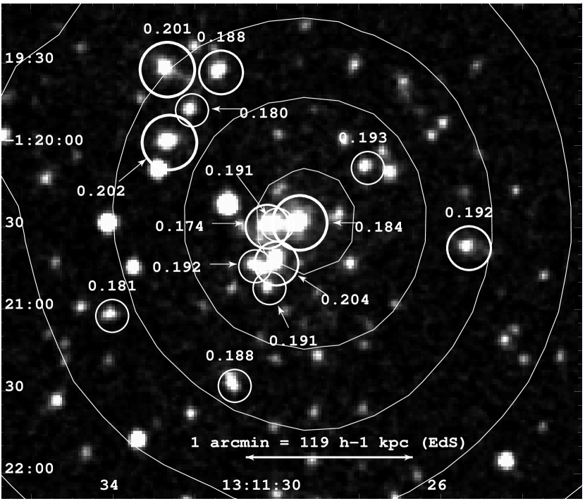
Figure 1.— R magnitude image of Abell 1689 from the STScI Digitized Sky Survey with all magnitude $R<18$ cluster members within the central $2^{\prime}$ region plotted over logarithmic X-ray contours from XMM Mos. The bump toward northeast is due to a foreground point source. Circle sizes are proportional to galaxy R magnitudes.

Abell 1689 is a cluster showing a large discrepancy among various mass determinations, and we chose it for a detailed study. It is a rich cluster, $R=4$, without a pronounced cooling flow but with an approximately circular surface brightness distribution suggesting a relatively relaxed structure. The large mass, $\sim 10^{15}~{}\mathrm{M_{\sun}}$ (Tyson & Fischer, 1995), and apparent symmetric distribution of Abell 1689 make it a suitable cluster for gravitational lensing measurements as well as X-ray measurements. However, the type of clusters that are believed to be the most relaxed have a cool central component of enhanced surface brightness. The absence of such a component in Abell 1689 suggests that the cluster is not fully relaxed. Also, the galaxy content of the cluster is unusually spiral rich for a cluster with high spherical symmetry and richness, with a galaxy type ratio E : S0 : Sp of approximately 22 : 22 : 28 plus 25 unidentified galaxies (Duc et al., 2002). Teague, Carter, & Gray (1990) measure a velocity dispersion of $\sigma_{1D}=2355^{+238}_{-183}~{}\mathrm{km~{}s^{-1}}$ for 66 cluster members, unusually high for a cluster of this temperature. Positions and redshifts from Duc et al. (2002) for all cluster members with red magnitude $R<18$ and within $2^{\prime}$ of the brightest central galaxy are shown in Fig. 1 together with logarithmic X-ray intensity contours from XMM Mos 1.

The gravitational lensing estimate from 6000 blue arcs and arclets calibrated by giant arcs at the Einstein radius of Abell 1689 gives a best fit power-law exponent of $n=-1.4\pm 0.2$ for the projected density profile from $200~{}h^{-1}~{}\mathrm{kpc}$ to $1~{}h^{-1}~{}\mathrm{Mpc}$ (Tyson & Fischer, 1995). (Unless otherwise stated, we assume an Einstein-deSitter (EdS) cosmology with $\Omega_{M}=1.0,\Omega_{\Lambda}=0.0$ and $H_{0}=100~{}h~{}\mathrm{km~{}s^{-1}~{}Mpc^{-1}}$.) This is steeper than the profile of an isothermal sphere $(n=-1)$. The strong lensing analysis of two giant arcs directly gives $M_{2D}(<0.10~{}h^{-1}~{}\mathrm{Mpc})=1.8\pm 0.1\times 10^{14}~{}h^{-1}~{}\mathrm{M_{\sun}}$ (Tyson & Fischer, 1995).

The mass profile derived from the deficit of lensed red galaxies behind the cluster due to magnification and deflection of background galaxies suggests a projected mass profile of $M_{2D}(<R)\approx 3.5\times 10^{15}(R~{}/~{}h^{-1}\mathrm{Mpc})^{1.3}~{}h^{-1}~{}\mathrm{M_{\sun}}$ for $R<0.32~{}h^{-1}~{}\mathrm{Mpc}$, close to that of an isothermal sphere $(M_{2D}\propto R)$. The mass interior to $0.24~{}h^{-1}~{}\mathrm{Mpc}$ from this method is $M_{2D}(<0.24~{}h^{-1}~{}\mathrm{Mpc})=1.8\pm 0.1\times 10^{14}~{}h^{-1}~{}\mathrm{M_{\sun}}$ (Taylor et al., 1998). Measurement of the distortion of the luminosity function due to gravitational lens magnification of background galaxies gives $M_{2D}(<0.25~{}h^{-1}~{}\mathrm{Mpc})=0.48\pm 0.16\times 10^{15}~{}h^{-1}~{}\mathrm{M_{\sun}}$ (Dye et al., 2001). Finally, the weak gravitational shear of galaxies in a ESO/MPG Wide Field Imager $33^{\prime}\times 33^{\prime}$ image gives a mass profile with best fit NFW profile with $r_{200}=1.14~{}h^{-1}~{}\mathrm{Mpc}$ and $c=4.7$ or a best fit SIS with $\sigma_{1D}=1028^{+35}_{-42}~{}\mathrm{km~{}s^{-1}}$ (Clowe & Schneider, 2001; King, Clowe, & Schneider, 2002).

There is a good indication from the optical data that the cluster consists of substructures. Miralda-Escudé & Babul (1995) suggest a strong lensing model with two clumps in order to reproduce the positions of the brightest arcs. A larger mass clump $(\sigma_{r}=1450~{}\mathrm{km~{}s^{-1}})$ is centered on the brightest cluster galaxy while a smaller clump $(\sigma_{r}=700~{}\mathrm{km~{}s^{-1}})$ is located $1^{\prime}$ northeast of the main clump. They arrive at a mass a factor 2 - 2.5 lower for their X-ray estimate compared to their gravitational lensing model. Girardi et al. (1997) identify two distinct substructures centered on redshifts $z=0.175$ and $z=0.184$ using positional and redshift data of cluster galaxies from Teague et al. (1990), providing further evidence that the cluster is not relaxed. These clumps are also aligned in the southwest – northeast direction but the locations do not agree with the ones of Miralda-Escudé & Babul (1995). Both structures are found to have $\sigma_{r}\sim 300-400~{}\mathrm{km~{}s^{-1}}$ yielding virial masses several times smaller than those derived from lensing and X-ray estimates.

Can the X-ray observations provide any evidence for a substructure in Abell 1689, and what are the implications on the mass inferred from the X-ray data? In an attempt to answer this, we analyze XMM-Newton EPIC pn and EPIC Mos data to measure the mass profile of A1689 and to investigate the spatial structure of the cluster. §2 contains the details of the observations and data reduction with the XMM-Newton as well as with summary of the ROSAT, Asca and Chandra data; §3 covers the methods of spectral fitting of the XMM data and presents the analysis of cluster asymmetry; §4 derives the mass and the slope of the mass distribution in the core; and §5 presents the inferences about the structure of the cluster inferred from the spatial analysis. The paper concludes with the summary in §6.

2. Abell 1689 X-ray observations

2.1. XMM-Newton observation

2.1.1 Data preparation

Abell 1689 was observed with XMM-Newton for 40 ks on December 24th 2001 during revolution 374. For imaging spectroscopy we use data from the European Photon Imaging Camera (EPIC) detectors Mos1, Mos2 and pn. Both Mos cameras were operating in the Full Frame mode whereas pn was using the Extended Full Frame mode. The Extended Full Frame mode for pn is appropriate for studying diffuse sources since it has lower time resolution and so it is less sensitive to contamination from photons being detected during readout of the CCDs. These events (so called Out-Of-Time events) show up as streaks across the X-ray image and are especially bothersome when the goal of an observation is spatially resolved spectroscopy of diffuse sources. All cameras used the Thin filter during the observation.

EPIC background is comprised mainly of three components. The external particle background consists primarily of soft protons $(E_{p}<100~{}\mathrm{keV})$ being funneled through the mirrors and causing a time variable flaring signal in the detector. The internal particle background is mainly due to high energy particles interacting with the detector material and causing a roughly flat spectrum with flourescent emission-lines characteristic to the detector material. This component varies over the detector surface. The third source of background is the cosmic X-ray background (CXB) which is roughly constant in time but varies over the sky.

For all data reduction we use the software and calibration data implemented in XMM Science Analysis Software (SAS) 5.4.1. To exclude the events contaminated by proton flares, we produce light curves in the $10-15~{}$keV band where the true X-ray signal is low. We screen the data using a constraint on the total count rate of less than 1.5 ct s^-1 for Mos and 1.1 ct s^-1 for pn in this band, leaving an effective exposure time of 37 ks for Mos and 29 ks for pn. This screening corresponds to a limit on the count rate of approximately $2\sigma$ above the quiescent period in the $0.3-10~{}$keV band.

2.1.2 Vignetting correction

The effective mirror collecting area of XMM-Newton is not constant across the field of view: it decreases with increasing off-axis angle and this decrease is energy dependent. This results in a position dependent decrease in the fraction of detected events and when doing imaging spectroscopy for extended sources, we need to account for this effect. By generating an Ancillary Response File (ARF) for each source spectrum region, using XMM SAS 5.4.1 command arfgen we calculate an average effective area for each region considered by us (see below).

2.1.3 Background subtraction

In order to correctly account for particle-induced and Cosmic X-ray Background, it would be optimal to extract a background spectrum from the same detector region collected at the same time as the source spectrum. This is of course impossible, and the background can be taken from a source-free region of the detector (other than the target, but near it), or can be estimated using blank sky data. We adopt the former method, noting that the background is not entirely constant over the field of view; however, it can be assumed to be approximately constant with the exception of the fluorescent Cu line at $8~{}\mathrm{keV}$ in pn which is the strongest contaminant emission line. Using this assumption, we can effectively subtract the particle background by extracting a spectrum in a source free region in the same exposure. For pn data in the $7.8-8.2~{}\mathrm{keV}$ range is excluded due to the strong spatial dependence of the Cu internal emission.

Using an ARF generated for a source region on a background subtracted spectrum will not take into account that the spectrum used as background was extracted from a different region where the vignetting was higher, due to the larger off-axis distance of the background region. This will have the effect that the CXB component in our source spectrum will be under-subtracted and the net spectrum will contain some remnant of the CXB. The particle induced background however is not vignetted and therefore should leave no remnant.

To estimate the CXB component in our exposure we take the events outside of the field-of-view to be the particle background. Another spectrum is then extracted from a large source free area, located away from the cluster. The particle background is normalized and removed from this spectrum. The resulting spectrum is fitted to a broken power law model to determine the CXB flux. The incorrect vignetting correction of the CXB is found to cause an at most 2 % over-estimation of the flux which is the case in the outermost annulus in our analysis (see below). However since the vignetting is energy-dependent, the incorrect vignetting may cause a small ($\sim 0.3$ keV) shift in temperature for the outermost region. The overall uncertainty in the background is estimated to be at most a few percent.

We compare our background subtraction method with the method of using XMM standard blank sky data compiled by Lumb (2002); we find that both methods give similar fit parameters. However, given the difficulty of normalizing the CXB, the different high-energy leftovers from proton-flare subtraction and the different internal particle background which occurs when using background data from a different exposure, we chose to use in-field (rather than blank-sky) background. We find this is more robust in keeping the overall shape of the source spectrum uncontaminated. In all our analysis we use a background region of a circular annulus with inner and outer radii of $6^{\prime}$ and $8^{\prime}$ respectively. In fact, recent work by Lumb et al. (2003) suggests that the in-field background method is probably more accurate. The clusters in the above paper, however, have smaller apparent angular size which makes the background method more reliable.

Figure 2.— Best fit MEKAL models for the XMM Mos (Left) and pn (Right) data from the central $3^{\prime}$ region of Abell 1689. The absorbing column was fixed at the galactic value (Dickey & Lockman, 1990).

2.1.4 Spectral fitting

In analyzing the vignetting corrected, background subtracted radial count-rate profile, we fit it to a conventional beta model, $S(r)\propto(1+r/r_{c})^{-3\beta+0.5}$, where $S(r)$ is the source surface brightness at radius $r$. The fit gives $r_{c}=91.2\pm 0.7~{}h^{-1}~{}\mathrm{kpc}$ and $\beta=0.72\pm 0.01$ with $\chi^{2}/dof.=46$ using data out to $700~{}h^{-1}~{}\mathrm{kpc}$. Clearly this model is not a very good fit; we show it here only for completeness and comparison with previous work, and note that it is not used in the subsequent analysis. The bad fit above results from the fact that the cluster emission is more peaked in the core than the best fit beta model. To obtain a general idea of the properties of the cluster and compare this with previous results, we extracted spectra for the central $3^{\prime}$ $(356~{}h^{-1}~{}\mathrm{kpc})$ region, centered on the X-ray centroid at $13^{h}11^{m}29^{s}.4$ $-01^{\circ}20^{\prime}28^{\prime\prime}$. This radius corresponds to $0.32~{}r_{200}$ or $3.9~{}r_{c}$. Background spectra were extracted from source-free regions from the same exposure. For XMM pn we use single and double pixel events only whereas for XMM Mos we also use triple and quadruple pixel events.

For spectral fitting we use the XSPEC (Arnaud, 1996) software package. We fit the data in the $0.3-10.0~{}\mathrm{keV}$ range using the MEKAL (Mewe, Gronenschild, & van den Oord, 1985; Mewe, Lemen, & van den Oord, 1986; Kaastra, 1992; Liedahl, Osterheld, & Goldstein, 1995) model for the optically thin plasma and galactic absorption. With the absorption fixed at the Galactic value, $N_{H}=1.8\times 10^{20}$ cm^-2 (Dickey & Lockman, 1990), and assuming a redshift $z=0.183$ we arrive at a temperature of $9.35\pm 0.17~{}\mathrm{keV}$ and a metal abundance of $0.27\pm 0.03$ Solar for both Mos cameras with $\chi^{2}/\mathrm{dof.}=951/824$. From the pn camera we get $8.25\pm 0.15~{}\mathrm{keV}$ and $0.23\pm 0.03$ Solar with $\chi^{2}/\mathrm{dof.}=1424/863$. The best fit models with residuals can be seen in Fig. 2 for Mos (Left) and pn (Right). The pn temperature is in disagreement with Mos data and the reason for this effect can be seen from the residuals below 1 keV for pn (Fig. 2 (Right)). Fitting the pn data above 1 keV we get $9.33\pm 0.20~{}\mathrm{keV}$ and $0.24\pm 0.03$ Solar with $\chi^{2}/\mathrm{dof.}=892/722$, in better agreement with Mos. The temperature from Mos is in agreement with that found by Asca, $9.02^{+0.40}_{-0.30}~{}\mathrm{keV}$ (Mushotzky & Scharf, 1997). This observation does not suffer from pile-up, nor is the low energy spectrum sensitive to background subtraction. The background uncertainties below 1 keV for this pn spectrum are less than 1 % whereas the pn soft excess is sometimes higher than 10 %. The excess is certainly not background related. It is possible that the pn low-energy discrepancy can be due to incorrect treatment of charge collection at lower energies (S. Snowden, priv. comm.). To resolve the discrepancy between Mos and pn we decided to compare with Asca GIS/SIS, ROSAT PSPC and Chandra ACIS-I data.

Figure 3.— The ratio of the XMM Mos (Left) and pn (Right) spectra of Abell 1689 to the best fit model determined from the ROSAT and Asca analysis.

2.2. ROSAT, Asca and Chandra observations

Besides the discrepancy regarding the softest X-ray band for the Abell 1689 data between the Mos and pn detectors aboard XMM-Newton, the spectral fits to the Chandra data presented by Xue & Wu (2002) imply a higher absorbing column, $6.7\pm 1.5\times 10^{20}$ cm^-2 than the Galactic value of $1.8\times 10^{20}$ cm^-2 (Dickey & Lockman, 1990). Since such excess absorption is not commonly detected in X-ray data for clusters, this requires further investigation. To determine if there is indeed any additional component of absorption beyond that attributable to the Galactic column – and assess the reliability of the softest energy band of the pn vs. Mos data – we used the most sensitive soft ($<1$ keV) X-ray data for this cluster obtained prior to the XMM-Newton observations, collected by the ROSAT PSPC. The ROSAT observation conducted during July 18-24, 1992 (available from HEASARC) yielded 13.5 ks of good data. We extracted the ROSAT PSPC counts from a region $3^{\prime}$ in radius, centered on the nominal center of X-ray emission. For background, we selected a source-free region of the same PSPC image. Using these data over the nominal energy range 0.15 - 2.1 keV with the standard PSPC response matrix applicable to the observation epoch, we performed a spectral fit to a simple, single-temperature MEKAL model with soft X-ray absorption due to gas with Solar abundances, using the XSPEC package as above. In the fit we use metal abundances of 0.27 Solar obtained in the XMM Mos fit above. While the limited bandpass of ROSAT PSPC precludes an accurate determination of the temperature (the best fit value is $kT=4.3^{+1.2}_{-0.8}$ keV, 90% confidence regions quoted), the PSPC data provide a good measure of the absorbing column: the best value is $1.9\pm 0.3\times 10^{20}$ cm^-2, certainly consistent with the Galactic value. We note that the difference between the temperature inferred from the PSPC fit and that obtained from the XMM-Newton data as above is a result of the limited bandpass of the PSPC, located much below the peak of the energy distribution of the cluster photons. The measurement of the absorbing column, however, clearly indicates that the column inferred from the Chandra observation by Xue & Wu (2002) is not correct, and might be due to instrumental effects. We conclude that the absorbing column is consistent with the Galactic value.

To obtain further constraints on the absorbing column, we also used the Asca GIS and SIS data together with the PSPC data for an independent constraint on the continuum radiation in the fitting process. We performed standard extraction of data from all Asca detectors, also from a region from a region $3^{\prime}$ in radius for the source, and a source-free region of the same image for background. We performed a spectral fit simultaneously to data from the PSPC and four Asca detectors. To account for possible flux calibration differences, we let the normalization among all the different detectors run free. We used the energy range of $0.7-9.0~{}\mathrm{keV}$ and $0.5-8.5~{}\mathrm{keV}$ for the Asca GIS and SIS cameras respectively. Since Asca detectors (and in particular, the SISs) often return spectral fits with excess intrinsic absorption (Iwasawa, Fabian, & Nandra, 1999) we also let the absorbing column be fitted independently for the GIS, SIS and PSPC detectors. Temperature and metal abundances were tied together for all datasets in the fit. The optical redshift $z=0.183$ was used. The joint fit of ROSAT and Asca data gives us the best fit temperature of $9.1\pm 0.5$ keV and abundances of $0.25\pm 0.06$ Solar, in agreement with the values quoted by Mushotzky & Scharf (1997), and the absorption (for the PSPC data) $1.75\pm 0.08\times 10^{20}$ cm^-2, in agreement with the Galactic HI 21 cm data. We shall use this value for the absorption in the subsequent analysis.

This best fit ROSAT/Asca model was compared with the data from the same region in the XMM-Newton cameras giving an unfitted reduced $\chi^{2}$ of 1.39 for pn and 1.06 for both Mos cameras combined. The ratio of these spectra to the ROSAT/Asca model can be seen in Fig. 3. From this result we conclude that Mos low energy response is more consistent with previous data and subsequently, we choose to ignore all pn data below $1.1~{}\mathrm{keV}$. Re-fitting the XMM data from the above region using $0.3-10.0~{}\mathrm{keV}$ for Mos data and $1.1-10.0~{}\mathrm{keV}$ for pn leaving the absorbing column as a free parameter yields $n_{H}=1.08\pm 0.16\times 10^{20}$ cm^-2, a temperature of $9.43^{+0.16}_{-0.15}~{}\mathrm{keV}$ and metallicity of $0.26\pm 0.02$ Solar. While this fitted value of absorption is formally inconsistent with the Galactic and ROSAT-inferred values, this is a relatively small difference, which might be due to the slightly imperfect calibration of the Mos detectors or the assumption of isothermality made by us for this fit (since $T$ and $n_{H}$ are correlated in the fitting procedure). We note that using the ROSAT value for absorption will give us a somewhat lower measure on the temperature (see below).

Finally, we reduced the Chandra data for Abell 1689 using the most recent release of data reduction software; specifically, due to the degradation of the Chandra ACIS-I low-energy response correction for the charge transfer inefficiency (CTI) is necessary, and we applied this to the Chandra data. As of Chandra data analysis software package CIAO ver. 2.3 this correction can be applied in the standard event processing. It is also necessary to account for the ACIS excess low-energy absorption due to hydrocarbon contamination. We used the acisabs code for the correction to the auxiliary response function. The event grades used in the ACIS analysis were GRADE=0,2,3,4 and 6.

Figure 4.— The ratio of the Chandra ACIS-I spectra of Abell 1689 to the best fit model determined from the ROSAT and Asca analysis, before (Left) and after (Right) the acisabs correction. Data used for the spectrum include events with ACIS grades 0, 2, 3, 4, and 6.

The cluster was observed with the Chandra ACIS-I detector array at two separate occasions for $10~{}$ks each on 2000-04-15 and 2001-01-07. Spectra were extracted for the central $3^{\prime}$ region centered on the X-ray centroid at $13^{h}11^{m}29^{s}.4$ $-01^{\circ}20^{\prime}28^{\prime\prime}$ following the CIAO 2.3 Science Threads for extended sources. Fig. 4 shows the ratio of the combined Chandra data to the best fit model determined from ROSAT and Asca above. The left spectrum is before and the right after the acisabs correction. Fitting the corrected spectrum to an absorbed MEKAL model in the energy range 0.3 - 7.0 keV yields absorption of $1.7\pm 0.6\times 10^{20}$ cm^-2, a temperature of $12.4\pm 1.1$ keV and abundances of $0.34\pm 0.10$ Solar using the optical redshift z=0.183. The discrepant absorption found by Xue & Wu (2002) (using data 0.7 - 9.0 keV) is apparently corrected for by acisabs and the value is in agreement galactic absorption. However there is still a large discrepancy in temperature, which also can be seen from the high energy ends of Fig. 4. Part of this effect can possibly be attributed to the high energy particle background but more likely to uncorrected instrumental effects. Repeating all above steps for single pixel events only (GRADE=0) in order to achieve higher spectral accuracy gives us a best fit temperature of $7.2\pm 0.4$ keV. We cannot account for the differences between the two Chandra data sets (using GRADE=0 vs. GRADE=0,2,3,4 and 6 events) nor between the results of the Chandra and XMM spectral fits. We note here that the photon statistics resulting from the XMM observation is superior to that in the Chandra data, and since our analysis does not require the superior angular resolution of the Chandra mirror, we limit the analysis below to the XMM data.

3. Spectral analysis

3.1. Temperature and metallicity distribution for a spherically symmetric model

To obtain a radial profile of cluster gas temperature, abundance, and density, we first make the assumption that the cluster is spherical and that above properties are only functions of radius. For this, we divide the image of the cluster into 11 concentric annuli out to $5^{\prime}50^{\prime\prime}$ $(693~{}h^{-1}~{}\mathrm{kpc})$ centered on the X-ray centroid. For each annulus, we extract spectra from all EPIC cameras, and we set the inner and outer radii of each region by requiring that each annulus contains at least 9000 counts per each Mos camera and 13000 for pn. This allows us to derive a reliable estimate of temperature in each region. Point sources with intensities greater than $3\sigma$ over the average are excluded. The outer radii of the annuli are as follows: $15^{\prime\prime}$, $25^{\prime\prime}$, $35^{\prime\prime}$, $47.5^{\prime\prime}$, $60^{\prime\prime}$, $75^{\prime\prime}$, $95^{\prime\prime}$, $125^{\prime\prime}$, $165^{\prime\prime}$, $230^{\prime\prime}$ and $350^{\prime\prime}$.

Average cluster properties were determined using all annular spectra simultaneously out to $693~{}h^{-1}~{}\mathrm{kpc}$ ($0.61~{}r_{200}$, $7.6~{}r_{c}$) using the same spectral fitting procedures as in Section 2.1.4. We use the optical redshift of $z=0.183$ (Teague et al., 1990) and the line of sight absorption of $N_{H}=1.75\times 10^{20}~{}\mathrm{cm^{-2}}$ as measured from ROSAT data, and also consistent with the Galactic column density (Section 2.2). The mean temperature of the cluster is found to be $kT=9.00^{+0.13}_{-0.12}~{}\mathrm{keV}$ and the mean abundance $0.25\pm 0.02$ Solar. We note that leaving the redshift as a free parameter gives a best fit redshift $z=0.173\pm 0.003$ (90% confidence range) which is considerably less than measured via optical observations. Considering Mos and pn data separately gives $z=0.171\pm 0.002$ and $z=0.178\pm 0.003$ respectively.

In order to take into account the three-dimensional nature of the cluster we consider the spectrum from each of the 11 annuli to be a superposition of spectra from a number of concentric spherical shells intersected by the same annulus. The spherical shells have the same spherical radii as the projected radii of the annuli. We assume that each shell has a constant temperature, gas density and abundance. The volume for each annulus/shell intersection is calculated to determine how large a fraction of emission from each shell should be attributed to each annulus. Assigning a spectral model to each spherical shell we can simultaneously fit the properties of all spherical shells.

In practice we use the method of Arabadjis, Bautz, & Garmire (2002) where we have a matrix of $11\times 11$ MEKAL models with absorption in XSPEC. In the process of fitting the data in XSPEC, each datagroup (consisting of three data files: pn, Mos1 and Mos2 spectra for each annulus) is fitted using the same set of models. For the central annulus (the one with zero inner radius so it’s actually a circle), which will intersect all 11 spherical shells, we will need to apply 11 MEKAL models to represent these. This means that we have to apply 11 MEKAL models to each datagroup (annulus) with absorption where each model represents the properties of one spherical shell. The normalization of each shell model is set to be the ratio of the volume that shell occupies in the cylinder that is the annulus/shell intersection to the volume it occupies in the central annulus. Abundance and temperature are tied together for the models representing the same spherical shell. Of course not all annuli intersect every shell, and for those shells not intersected by the annulus to which they are attributed, the model normalization will be zero. The matrix of MEKAL models is thus triangular and can be fitted directly to the spectra we have extracted from annular regions in the data. This approach allows for all data to be fitted simultaneously, and we do not have the problem with error propagation which occurs when starting to fit the outermost annulus and propagating inward subtracting contributions from each previous shell.

Figure 5.— The radial metallicity distribution of Abell 1689 as derived from the spectral deprojection fitting.

The metallicity profile (Fig. 5) from the deprojection shows signs of increasing abundance toward the center of the cluster. In temperature (Fig. 6) we find an apparent decrease for large radii ($kT<8~{}\mathrm{keV}$), an effect that has been seen in analysis of other clusters with XMM (see e.g. Pratt & Arnaud (2002)). Gas dynamic simulations of the formation of galaxy clusters also show a decline of temperature at large radii (Evrard & Metzler, 1996). We do not find a significant cooling in the cluster core with the highest temperature ($kT\sim 9.5~{}\mathrm{keV}$) near the core radius: in fact, we will show in section 3.2 that the temperature profile is not symmetric around the cluster center. We note that for completeness, we also performed the above analysis with the best-fit value of the redshift inferred from the X-ray data alone, and while the exact values of temperature and elemental abundances are slightly different, about 0.2 keV lower for temperature, the general trends in the radial runs of the parameters are the same.

Figure 6.— The radial temperature distribution of Abell 1689 as derived from the spectral deprojection fitting.

The limited point spread function (PSF) of the XMM mirrors is a potential problem especially for the annuli located close to the center since those are not much larger than the PSF FWHM of $\sim 6^{\prime\prime}$. Some of the flux incident on the central (circular) region will be distributed over the outer annuli and vice versa. This flux redistribution will have the effect of smoothing out the measured temperature profile since all annuli will have some flux that originally belong in other annuli. This effect has been studied in detail by e.g. Pratt & Arnaud (2002) who find that correcting for the PSF redistribution gives a profile that is consistent with an uncorrected profile. Abell 1689 has a temperature profile without large temperature variations and no large central flux concentration. We conclude that the effect of flux redistribution in our case will be small and we do not attempt to correct for this. The PSF is also weakly energy dependent, and to quantify its possible effect on the observed temperature profile, we calculate the energy dependent flux loss from the central annulus and the effect on the central temperature. The difference in flux loss between various energy bands (ranging from 1.5 to 7.5 keV) for the on-axis PSF is $\sim 3\%$. We find that for a cluster with an assumed temperature of 9 keV, this could give an error of the central temperature by at the most $0.5~{}\mathrm{keV}$. We note that this is a maximum difference since in practice, the flux gained from outer annuli could somewhat reduce this effect by working in the opposite manner.

The luminosity of the cluster in the $0.5-10.0~{}\mathrm{keV}$ band, calculated from the best fit model above (with $z=0.183$) gives $L_{X~{}(EdS)}=1.02\times 10^{45}~{}h^{-2}~{}\mathrm{ergs~{}s^{-1}}$ for an EdS ($\Omega_{M}=1.0$, $\Omega_{\Lambda}=0.0$) Universe or $L_{X~{}(CDM)}=1.21\times 10^{45}~{}h^{-2}~{}\mathrm{erg~{}s^{-1}}$ for a CDM ($\Omega_{M}=0.3$, $\Omega_{\Lambda}=0.7$) Universe. This corresponds to a bolometric luminosity of $L_{bol~{}(EdS)}=1.63\times 10^{45}~{}h^{-2}~{}\mathrm{erg~{}s^{-1}}$ or $L_{bol~{}(CDM)}=1.94\times 10^{45}~{}h^{-2}~{}\mathrm{erg~{}s^{-1}}$. All above values should include 10% as the absolute calibration error of XMM. From Chandra analysis, Xue & Wu (2002) find $L_{bol(EdS)}=1.66\pm 0.64\times 10^{45}~{}h^{-2}~{}\mathrm{ergs~{}s^{-1}}$ whereas Mushotzky & Scharf (1997) find $L_{bol(EdS)}=1.77\times 10^{45}~{}h^{-2}~{}\mathrm{ergs~{}s^{-1}}$ from Asca data, both in agreement with our results. This does not provide any new information regarding the location of Abell 1689 in the Luminosity-Temperature (Mushotzky & Scharf, 1997) relation and it is still in a close agreement with the trend suggested by other clusters.

Table 1Comparison of the position of the cluster center of Abell 1689 from member galaxies, gravitational lensing and X-ray data

Method	Center		Ref.
	R.A. (J2000.)	Dec. (J2000.)
X-ray (ROSAT)	$13^{h}11^{m}29^{s}.1$	$-01^{\circ}20^{\prime}40^{\prime\prime}$	1
X-ray (Chandra)	$13^{h}11^{m}29^{s}.45$	$-01^{\circ}20^{\prime}28^{\prime\prime}.06$	2
Lensing	$13^{h}11^{m}29^{s}.6$	$-01^{\circ}20^{\prime}29^{\prime\prime}$	1
Optical	$13^{h}11^{m}29^{s}.44$	$-01^{\circ}20^{\prime}29^{\prime\prime}.4$	3
X-ray (XMM)	$13^{h}11^{m}29^{s}.4$	$-01^{\circ}20^{\prime}28^{\prime\prime}$	4

References. — (1) Allen (1998) ; (2) Xue & Wu (2002); (3) Duc et al. (2002); (4) This study.

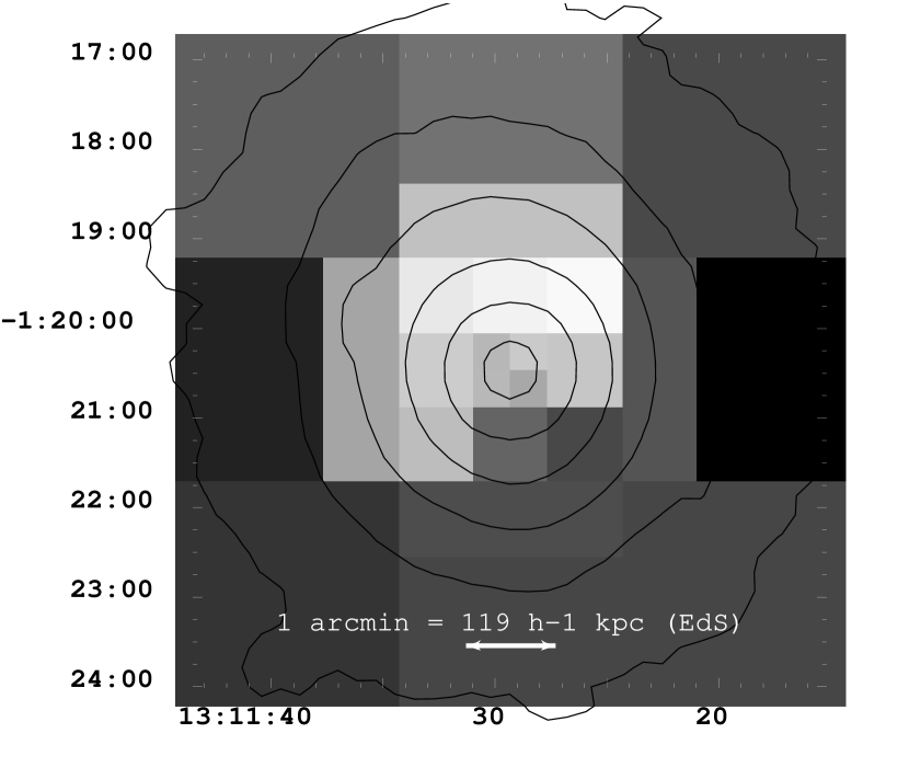
Figure 7.— Spatial distribution of spectral fit temperatures (6-10 keV) with superimposed logarithmic X-ray contours for A1689. 6 keV is marked as black, 10 keV is white, and intermediate temperatures are various shades of gray.

3.2. Asymmetry analysis

With the good quality XMM data, it is possible to verify the result of Xue & Wu (2002) that there is no discrepancy between the optical and X-ray centers of the cluster. We determine the center of X-ray emission for Abell 1689 using XIMAGE command centroid. We also include a measurement of the lensing center from Duc et al. (2002) and the X-ray measurement from ROSAT by Allen (1998) (Table 3.1). We find that all values agree within $3^{\prime\prime}$ except the ROSAT estimate, the offset of which we attribute to uncertainties in ROSAT HRI astrometry. This apparently perfect agreement among X-ray, lensing, and optical centers leads us to conclude that the ICM density peak and the central dominant galaxy is probably located at the bottom of the dark matter potential well. Still, the apparent non-uniformity of the ICM radial temperature distribution as well as the offset of optical and X-ray redshifts prompted us to analyze the spatial structure of the cluster. In Fig. 7 we show the spatial temperature distribution. Spectra were extracted in rectangular regions and fitted using the same method as in Section 2.1.4. The temperature in the figure scales linearly from 6 keV (black) to 10 keV (white). The errors on the temperature of the inner 16 regions are $\sim 0.5~{}\mathrm{keV}$, while the errors on the outer 8 regions are $\sim 1.0~{}\mathrm{keV}$. We clearly see an asymmetry in the temperature around the cluster center with an overall increase toward the northeast.

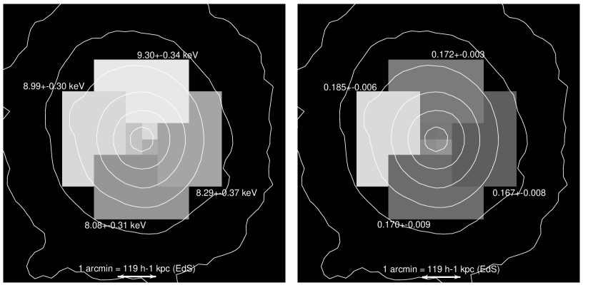
Figure 8.— The spatial distribution of temperature (left) and redshift (Right) in the central region of Abell 1689 with 90% confidence intervals.

To check the consistency of these results and to increase our accuracy, we re-group the data in larger spatial regions and perform a fit using the same above procedure. We first fit the data keeping the redshift frozen at the optical value. Temperatures derived from this fit are shown in Fig. 8 (Left). Thereafter, we leave the redshift as a free parameter and re-fit the data. The fitted redshifts for these regions are shown in Fig. 8 (Right). All errors in Fig. 8 are 90% confidence limits. In the temperature map, we see a clear discrepancy between the northern and southern part of the cluster with a hint of a temperature gradient in the southwest – northeast direction. The redshift map reveals a high redshift structure to the east at $z=0.185\pm 0.006$ separated from the rest of the cluster at $z\sim 0.17$. Analyzing the Mos and pn data separately for this high redshift region gives a broad minimum in $\chi^{2}$ at $z=0.187\pm 0.008$ for Mos whereas pn shows several minima in the $z=0.165-0.200$ range.

This region may indicate a subcluster falling inward away from the observer. This is further supported by the optical data, indicating that there are also high-redshift giant elliptical galaxies in this region (Fig. 1): it is interesting to speculate if this is actually the remains of a cluster core? Especially intriguing is the apparent coincidence between the smaller subcluster as suggested by strong lensing (Miralda-Escudé & Babul, 1995) and our high redshift gas region approximately $1^{\prime}$ northeast of the main cluster. Another possibility is that the redshift variation is due to large bulk motions of the intra-cluster gas. It has been shown in gas dynamic simulations that clusters with apparently relaxed X-ray profiles can have complex gas-velocity fields and be far from relaxed (Evrard & Metzler, 1996). This kind of motion could give rise to non-thermal emission from shocks etc. In our analysis we cannot distinguish between the two possibilities of bulk motion and subclustering.

This measurement of non-uniform redshift distribution of the X-ray emitting gas is important, and to verify if it could be due to instrumental effects, we investigated this in more detail. The data in the regions above are from different CCD chips in the pn data whereas for Mos all data are from the same chip. Since the pn camera provides about half of the data, we want to verify that there are no gain shifts between the CCDs, which, if present, could easily cause such an effect. Most of the cluster emission is on the CCD chips 4 and 7. To test for any possible gain offset, we extracted the data from each of the chips individually to verify the position of the internal fluorescent $\mathrm{CuK}\alpha$ line, with the dominant component at $8.0478~{}\mathrm{keV}$. The spectra in the range $7.8-8.2~{}\mathrm{keV}$ are fitted to a Gaussian profile: both datasets yield essentially the same peak position of $8.051\pm 0.001~{}\mathrm{keV}$. This corresponds to a possible artificial redshift offset of maximum $\Delta z=0.0005$. To explain the difference in the offset measured by us as an instrumental effect, we would have to have an offset (say at the Fe K line at 6.7 keV) of 62 eV, and not on the order of 1 eV, as inferred from the Cu K instrumental line. Hence we conclude that there is no gain shift that could alter our redshift measurements between pn CCDs 4 and 7. According to XMM calibration documentation (Kirsch, 2003) the magnitude of calibration errors for pn & Mos should be no larger than 10 eV.

4. Mass Profile

4.1. Mass calculation

If we assume that the cluster is spherical with a smooth static gravitational potential and that the intra-cluster medium is a pressure-supported plasma, we can employ the hydrostatic equilibrium equation. The circular X-ray isophotes (Fig. 1) generally indicate that a cluster is in dynamical equilibrium. The hydrostatic equation can be written as (Sarazin, 1988) :

$$M(r)=-\frac{kT_{g}(r)~{}r}{Gm_{p}\mu}\left(\frac{\mathrm{d}~{}ln~{}T_{g}(r)}{\mathrm{d}~{}ln~{}r}+\frac{\mathrm{d}~{}ln~{}\rho_{g}(r)}{\mathrm{d}~{}ln~{}r}\right)$$ (1)

where $M(r)$ is the enclosed total gravitating mass enclosed within a sphere of a radius $r$, $T_{g}(r)$ and $\rho_{g}(r)$ are temperature and density of the ICM at $r$, $\mu$ is the mean particle weight and $m_{p}$ is the proton mass. Using the temperature and normalizations from the spectral deprojection fitting we calculate the total gravitating mass. Errors are treated by error propagation.

The mass distribution is fitted to a singular isothermal sphere (SIS)

$$M(r)=\frac{2\sigma_{r}^{2}r}{G}$$ (2)

where $\sigma_{r}$ is the 1-dimensional velocity dispersion, which is used here for a comparison with previous mass estimates.

The predicted density profile from CDM hierarchal clustering according to Navarro et al. (1997) for dark matter halos is

$$\frac{\rho(r)}{\rho_{crit}(z)}=\frac{\delta_{c}}{(r/r_{s})(1+r/r_{s})^{2}}$$ (3)

where $\rho_{crit}(z)$ is the critical energy density at halo redshift $z$ and $\delta_{c}$ is characteristic density defined by

$$\delta_{c}=\frac{200}{3}\frac{c^{3}}{[ln(1+c)-c/(1+c)]}$$ (4)

where $c=r_{200}/r_{s}$ is the concentration of the halo defined as the ratio of the virial radius $r_{200}$ to $r_{s}$, which in turn is a characteristic radius in the NFW model. The critical density at redshift $z$ for a flat ($\Omega_{0}=1$) Universe is

$$\rho_{crit}(z)=\frac{3H_{0}^{2}}{8\pi G}[\Omega_{M}(1+z)^{3}+\Omega_{\Lambda}]$$ (5)

where $H_{0}$ is the Hubble constant, $\Omega_{M}$ and $\Omega_{\Lambda}$ are the current contributions of matter and vacuum energy respectively to the energy density of the Universe.

More recent numerical studies suggest a steeper core slope and a sharper turn-over from small to large radii (Moore et al, 1999). Both models can be generalized as

$$\rho(r)=\frac{\rho_{0}}{(r/r_{s})^{\gamma}[1+(r/r_{s})^{\alpha}]^{(\beta-\gamma)/\alpha}}$$ (6)

(Zhao, 1996), where $\gamma$ and $\beta$ characterize the density slope at small and large radii respectively whereas $\alpha$ determines the sharpness in the turn-over. Most studies agree on $\beta=3$ but the value of $\gamma$ is still being debated. The NFW and Moore profiles fit into the parameter space $(\alpha,\beta,\gamma)$ as $(1,3,1)$ and $(1.5,3,1.5)$ respectively.

We choose to fit our data to the NFW model (Eq. 3) which, when integrated over $r$, yields

$$M(r)=M_{0}\times[\ln(1+r/r_{s})+(1+r/r_{s})^{-1}-1]$$ (7)

where $M_{0}=4\pi\rho_{c}\delta_{c}r_{s}^{3}$. We find that the data give the best fit for the NFW model with $c=7.2^{+1.6}_{-2.4}$ and $r_{200}=1.13\pm 0.21~{}h^{-1}~{}\mathrm{Mpc}$ whereas the SIS fit gives $\sigma_{r}=918\pm 27~{}\mathrm{km~{}s^{-1}}$. The total mass data and models are shown in Fig. 9 together with the mass of the X-ray emitting gas $M_{gas}$. Model parameters are summarized in Table 2. For a cosmology with $\Omega_{M}=0.3$ and $\Omega_{\Lambda}=0.7$, the best fit NFW model changes to $c=7.7^{+1.7}_{-2.6}$ and $r_{200}=1.31\pm 0.25~{}h^{-1}~{}\mathrm{Mpc}$.

Figure 9.— Spherical mass profile of Abell 1689 (pluses) with best fit NFW model (solid line) and singular isothermal sphere model (dot-dashed). The singular isothermal sphere is clearly not a very good fit to the data (see also Table 2). For comparison, the mass of the intra-cluster gas is included (asterisks).

Another cosmologically important quantity for clusters is the fraction of the total mass that is in the X-ray emitting gas, $f_{gas}=M_{gas}/M_{TOT}$. Allen et al. (2003) analyze data from the Chandra Observatory for 10 dynamically relaxed clusters between $z=0.09$ and $z=0.46$ and measure an average redshift independent $f_{gas}=0.108\pm 0.014$ at the $r_{2500}$ radius (where the total mass density is 2500 times the critical density at the redshift of the cluster). The cosmology where this is valid is a flat $\Lambda\mathrm{CDM}$ cosmology with $\Omega_{M}=0.291^{+0.040}_{-0.036}$ assuming $\Omega_{b}~{}h^{2}=0.0205\pm 0.0018$ and $h=0.72\pm 0.08$. The error on $f_{gas}$ above is the rms dispersion of the Allen et al. (2003) sample which is comparable to the individual errors on $f_{gas}$. With our best fit NFW model in the above cosmology we find $f_{gas}=0.072\pm 0.008$ for Abell 1689 at the $r_{2500}$ radius. This is lower than all the clusters in the Allen et al. (2003) sample and significantly lower than the mean. We find that in our estimate $f_{gas}$ has not converged to a constant and this might help explain part of the discrepancy. However, it may be the case that for many clusters $f_{gas}$ does not converge until well beyond $r_{2500}$.

Table 2Best fit models for the total mass profile of Abell 1689

Model	Range $[h^{-1}\mathrm{kpc}]$	Parameters	$\chi^{2}$ (dof.)
$\mathrm{NFW}_{EdS}$	$20-500$	$c=7.2~{}r_{200}=1.13~{}h^{-1}~{}\mathrm{Mpc}$	7.64 (8)
$\mathrm{NFW}_{CDM}$	$20-500$	$c=7.7~{}r_{200}=1.31~{}h^{-1}~{}\mathrm{Mpc}$	7.64 (8)
SIS	$20-500$	$\sigma=918~{}\mathrm{km~{}s^{-1}}$	61.4 (9)
POW	$20-90$	$\gamma=1.73\pm 0.34$
POW	$200-500$	$\gamma=0.72\pm 0.32$

Note. — The singular isothermal sphere (SIS) and powerlaw (POW) models are not quoted for different cosmologies since they are independent of cosmological parameters.

Comparing the mass and temperature at $r_{2500}$ of Abell 1689 to the M-T relation derived for a set of relaxed clusters (Allen & Fabian, 2001) shows a low mass for the temperature of Abell 1689. The M-T relation predicts $H(z)/H_{0}\times M_{2500}=4.5\times 10^{14}\mathrm{M_{\sun}}(\pm 10\%)$ for a $9~{}\mathrm{keV}$ cluster where $H(z)$ is the Hubble constant at the redshift of the cluster. For Abell 1689 we find $H(z)/H_{0}\times M_{2500}=2.4\times 10^{14}\mathrm{M_{\sun}}(\pm 15\%)$, significantly lower. The above values were derived assuming a flat $\Lambda\mathrm{CDM}$ cosmology with $\Omega_{M}=0.3$, $\Omega_{\Lambda}=0.7$ and $h=0.7$. The unusually low mass may be due to the fact that the mass of Abell 1689 seems to increase steadily beyond $r_{2500}$. However, we note that a lower mass (than would be predicted by the M-T relation) is not an uncommon feature for unrelaxed clusters (cf. Smith et al. (2003)).

For completeness, we note that the calculated total mass includes the ICM and galaxy mass contributions as well as the dark matter. The proper way of fitting the NFW model would be to subtract these contributions prior to performing the fit. The NFW model for the actual dark matter halo is not used in this paper; we only calculate the total mass profile.

4.2. Core slope

The mass data were fitted to a simple power law ($M(<r)\propto r^{\gamma}$) in the ranges $20-90~{}h^{-1}~{}\mathrm{kpc}$ and $200-500~{}h^{-1}~{}\mathrm{kpc}$. We find the best fit of the slope of the matter profile to to be $1.73\pm 0.34$ and $0.72\pm 0.32$ for small and large radii, respectively. This corresponds to total mass density slopes ($\rho\propto r^{\alpha}$) of $\alpha=-1.27\pm 0.34$ and $\alpha=-2.28\pm 0.32$, in good agreement with what is expected from numerical simulations of CDM hierarchal clustering. We note here that Bautz & Arabadjis (2002) have measured the density profile of Abell 1689 for $r<100~{}h^{-1}~{}\mathrm{kpc}$ using Chandra data and found $\alpha\sim-1.3$.

We do not observe a flattening of the core density profile but find a slope close to the core to be somewhere in between the preferred Moore and NFW profiles. Thus we do not claim to be able to detect nor dismiss any kind of modification to standard cold dark matter. Nonetheless, the X-ray data imply an upper limit on the self-interaction of dark matter; see, e.g., the discussion in Arabadjis et al. (2002). Such comparisons are more meaningful for cooling-flow clusters which are presumably more relaxed objects.

5. Discussion

5.1. Comparison with Lensing

To compare our results with those obtained from gravitational lensing, we reprojected our derived mass distribution into a two dimensional distribution by summing up the contributions from each shell along the line-of-sight. Of course this method assumes that the outermost shell is the absolute limit of the cluster, and we recognize that this will not be entirely accurate. Therefore we also include our projected best-fit NFW model which has an analytic expression. Reprojected mass and NFW model are shown in Fig. 10 where pluses with error bars are the reprojected mass, the solid line is our NFW model, the triangle is the strong lensing result (Tyson & Fischer, 1995), the asterisks are lensing magnification results measured by the distortion of the background galaxy luminosity function (Dye et al., 2001), the dot-dashed lines are lensing magnification results measured by the deficit of red background galaxies (Taylor et al., 1998), and the dashed line is the best fit NFW model from weak gravitational shear analysis (Clowe & Schneider, 2001; King et al., 2002). The comparison of our results with measurements from gravitational lensing is summarized in Table 5.1.

Figure 10.— Unparameterized projected mass distribution, assuming that our the outermost shell is the limit of the cluster mass (pluses with errorbars), plotted with reprojected best fit NFW model (solid line). Also shown are gravitational lensing results from strong lensing (triangle), distortion of background galaxy luminosity function (asterisks), deficit in number counts of red background galaxies (dot-dashed lines) and projected best fit NFW model from weak gravitational shear (dashed line).

The X-ray mass appears to be in good agreement with that derived from weak gravitational shear but cannot be reconciled with the strong lensing data nor with the data from gravitational lens magnification. This discrepancy in lensing was noted earlier by Clowe & Schneider (2001) as well as King et al. (2002) who cannot find an agreement using any realistic corrections. The high velocity dispersion measured by Teague et al. (1990) and the apparent grouping of galaxies along the line of sight (Girardi et al., 1997) may indicate that this cluster is not as regular as we expect from its smooth circular surface intensity. The two component model of Miralda-Escudé & Babul (1995) also strongly suggests non-uniformity. This might explain the discrepancies between mass estimates from gravitational lensing and from X-rays. A possibility could be that this is a cluster undergoing a major merger, where a sub-clump close to or along the line-of-sight is being stripped from gas or just has very low X-ray luminosity.

Table 3Comparison of previous mass estimates from gravitational lensing to our X-ray estimate of Abell 1689

$M_{2D}~{}[10^{15}~{}h^{-1}~{}\mathrm{M_{\sun}}]$	Radius $[h^{-1}~{}\mathrm{Mpc}]$	Ref.	Type of Measurement
$0.18\pm 0.01$	$<0.10$	1	Strong lensing
$0.082\pm 0.013$	$<0.10$	4	X-ray
$0.50\pm 0.09$	$<0.24$	2	Weak lensing magnification
$0.48\pm 0.16$	$<0.25$	3	Weak lensing magnification
$0.20\pm 0.03$	$<0.25$	4	X-ray

References. — (1) Tyson & Fischer (1995) ; (2) Taylor et al. (1998); (3) Dye et al. (2001); (4) This study.

5.2. Large scale configuration

To illustrate the possible explanation that a merger might be taking place in this cluster and motivate why the X-ray derived mass should be lower than expected we employ a simple model. We assume that we have two perfectly spherical clusters aligned exactly along the line of sight having identical mass ($M_{1}$) and gas density ($n_{1}$). Since the thermal bremsstrahlung emissivity scales as $n^{2}$ we will measure a surface intensity $S(r)\propto n^{2}(r)$ and from this infer a gas density $n(r)$. In this example however we have $S(r)=2S_{1}(r)\propto 2n_{1}^{2}(r)$ and hence we will conclude that $n(r)=\sqrt{2}~{}n_{1}(r)$. This means that we underestimate the total mass of the X-ray emitting gas by a factor $\sqrt{2}$.

From the hydrostatic equation (Eq. 1) we can write $M(r)\propto\mathrm{d}(ln~{}n)/\mathrm{d}(ln~{}r)\propto n^{-1}~{}\mathrm{d}n/\mathrm{d}r$. From the gradient of the measured surface brightness $\mathrm{d}S/\mathrm{d}r\propto n(r)~{}\mathrm{d}n/\mathrm{d}r$ we infer a gradient on the gas density. In our scenario it is true that $\mathrm{d}S/\mathrm{d}r=2~{}\mathrm{d}S_{1}/\mathrm{d}r$ which yields $\mathrm{d}n/\mathrm{d}r=\sqrt{2}~{}\mathrm{d}n_{1}/\mathrm{d}r$. For the total mass we will measure $M(r)\propto n^{-1}~{}\mathrm{d}n/\mathrm{d}r=n_{1}^{-1}~{}\mathrm{d}n_{1}/\mathrm{d}r$. The actual mass of the cluster pair is of course $2~{}M_{1}$ which is twice what we measure. We have underestimated the total gravitating mass by a factor $2$. This is in agreement what we find in our comparison with gravitational lensing derived masses which would be able to measure the total mass accurately in this example.

While this exact scenario is not very probable it shows that a close configuration of clusters will underestimate the X-ray mass, maybe by a factor as large as 2. In the above example the gas mass fraction would actually be overestimated which is the opposite of what we find. However if a merger was in fact taking place the hydrostatic equation would probably be quite inaccurate estimation of the mass. There would be other sources of pressure and probably the cluster would not be in equilibrium: examples here might be magnetic fields, or additional pressure support from non-thermal particles, likely to be accelerated in shocks that arise during a merger. Also since we do not detect two separate peaks in the surface intensity map, it is much more likely we have a lower density companion cluster or one merging irregular system.

5.3. The dynamical state of Abell 1689

There is a good evidence suggesting that Abell 1689 is undergoing a merger. We find that the X-ray measurement yields the value of mass that is low in comparison to gravitational lensing and the M-T relation for relaxed clusters, both by about a factor 2. We have shown that this may be the result of grouping or elongation along the line of sight. The cluster has a low gas mass fraction compared to other clusters, which is perhaps the result of large scale gas motion. The velocity dispersion of the member galaxies is very high and there are hints of subgroupings in the redshift space. The high number of spiral galaxies is unusual for a rich cluster and suggests a lower density region, where the spiral fraction would be higher, perhaps in front of or behind the main cluster. A state of complex dynamics is supported by the non-uniform temperature distribution and maybe most importantly by the variation in redshift of the X-ray emitting gas across the cluster. Finally, recent measurements of the Sunyaev-Zeldovich effect by Benson et al. (2004) indicate that the inferred optical depth of the Comptonizing gas might actually be higher than one would infer from the simple spherically symmetric model obeying hydrostatic equilibrium, and a clumpy or elongated structure (aligned along the line of sight) would alleviate the discrepancy.

Clearly, this cluster deserves further detailed studies; it is a very interesting potential target for the Astro-E2 mission, where the X-ray calorimeter will provide an unprecedented spectral resolution, capable of clearly confirming the complex redshift structure of the intra-cluster gas, hinted by the XMM data. If the cluster is indeed undergoing a merger, this might provide an environment where at least some fraction of the gas is accelerated (for instance, via shocks) to form a non-thermal distribution of particles, which might produce radiation detectable in radio (via synchrotron emission), in hard X-rays (by Comptonizing the Cosmic Microwave Background), and in gamma rays, potentially detectable by the future mission GLAST.

6. Summary

The superior effective area of the XMM-Newton telescope has allowed us to perform a detailed analysis of Abell 1689. Comparing with the data from ROSAT, Asca and Chandra we verified that the data are consistent with earlier observations. Importantly, there is no indication of any additional absorbing component in the XMM data, attributing the low-energy excess absorption found by Xue & Wu (2002) in the Chandra data to uncorrected instrumental effects. The now available acisabs code successfully corrects for these effects. We confirm earlier findings that there is a large discrepancy, of a factor 2 or more, between mass estimates from gravitational lensing and X-ray derived mass using an unparameterized deprojection technique. Our analysis indicates that this discrepancy is true for the central part of the cluster, but also might be the case for the entire observable cluster; our finding is in contrast to Xue & Wu (2002), who conclude that at large radii, there is no disagreement between the X-ray and lensing masses. Although the X-ray determined mass appears to be discrepant from the values determined from most lensing techniques, it seems to be in good agreement with that derived from weak gravitational shear. We compare the gas mass of the cluster with the total mass, and find that for Abell 1689, $f_{gas}=M_{gas}/M_{TOT}$ is $0.072\pm 0.008$, significantly less than $0.108\pm 0.014$, the value derived by Allen et al. (2003) for 10 dynamically relaxed clusters. Our calculation of the asymmetric temperature distribution of the cluster provides further evidence that this cluster is not in a relaxed state: the lower than expected gas mass fraction is yet another piece of evidence. We also present the first measurement of asymmetries in redshift for different regions of the ICM in the cluster determined from the X-ray data alone. A similar analysis was done by Dupke & Bregman (2001) who claim a 3-$\sigma$ detection of bulk motion from Asca observations of the Centaurus cluster. We argue that the redshift variation detected here might be either due to line-of-sight clustering or possibly due to large bulk motions of the gas. Even though this cluster is clearly not as relaxed as might be expected from its apparent spherical form, we find the slope of the total mass in the central region to be in good agreement with what is expected from numerical simulations of structure formation. The density slope for $r<90~{}h^{-1}~{}\mathrm{kpc}$ is $-1.3$. While our current understanding of the structure and dynamics of galaxy clusters is insufficient to put limits on the self-interaction of dark matter, better data and more accurate simulations appear promising for the future.

References

- Allen (1998) Allen, S. W. 1998, MNRAS, 296, 392
- Allen & Fabian (2001) Allen, S. W, & Fabian, A. C. 2001, MNRAS, 328, L37
- Allen et al. (2003) Allen, S. W., Schmidt, R. W., Fabian, A. C., & Ebeling, H. 2003, MNRAS, 342, 287
- Arnaud (1996) Arnaud, K. A. 1996, in ASP Conf. Ser. 101, Astronomical Data Analysis Software and Systems V, ed. G. H. Jacoby & Jeannette Barnes (San Francisco: ASP), 17
- Arabadjis et al. (2002) Arabadjis, J. S., Bautz, M. W., & Garmire, G. P. 2002, ApJ, 572, 66
- Bautz & Arabadjis (2002) Bautz, M. W., & Arabadjis, J. S. 2002, AAS, 201, 0303A
- Benson et al. (2004) Benson, B., et al. 2004, submitted to ApJ
- Clowe & Schneider (2001) Clowe, D., & Schneider, P. 2001, A&A, 379, 384
- Dickey & Lockman (1990) Dickey, J. M., & Lockman, F. J. 1990, ARA&A, 28, 215
- Duc et al. (2002) Duc, P.-A., Poggianti, B.M., Fadda, D., Elbaz, D., Flores, H., Chanial, P., Franceschini, A., Moorwood, A., & Cearsky, C. 2002, A&A, 382, 60
- Dupke & Bregman (2001) Dupke, R. A., & Bregman, J. N. 2001, ApJ, 562, 266
- Dye et al. (2001) Dye, S., Taylor, A. N., Thommes, E. M., Meisenheimer, K., Wolf, C., & Peacock, J. A. 2001, MNRAS, 321, 685
- Evrard & Metzler (1996) Evrard, A. E., & Metzler, C. A. 1996, ApJ, 469, 494
- Girardi et al. (1997) Girardi, M. et al. 1997, ApJ, 490, 56
- Smith et al. (2003) Smith, G. P., Edge, A. C., Eke, V. R., Nichol, R. C., Smail, I., & Kneib, J.-P. 2003, ApJ, 590, L79
- Iwasawa, Fabian, & Nandra (1999) Iwasawa, K., Fabian, A. C., & Nandra K. 1999, MNRAS, 307, 611
- Kaastra (1992) Kaastra, J. S. 1992, An X-Ray Spectral Code for Optically Thin Plasmas (Internal SRON-Leiden Report, updated version 2.0)
- Kauffman, White, & Guiderdoni (1993) Kauffman, G., White, S. D. M., & Guiderdoni, B. 1993, MNRAS, 264, 201
- King et al. (2002) King, L. J., Clowe, D. I., & Schneider, P. 2002, A&A, 383, 118
-
Kirsch (2003)
Kirsch, M. 2003, EPIC status of calibration and data analysis, XMM-SOC-CAL-TN-0018, available from
http://xmm.vilspa.esa.es/docs/documents/ - Liedahl, Osterheld, & Goldstein (1995) Liedahl, D. A., Osterheld, A. L., & Goldstein, W. H. 1995, ApJ, 438, L115
-
Lumb (2002)
Lumb, D.H. 2002, EPIC Background Files, XMM-SOC-CAL-TN-0016, available from
http://xmm.vilspa.esa.es/docs/documents - Lumb et al. (2003) Lumb D. H., Bartlett, J. G., Romer, A. K., Blanchard, A., Burke, D. J., Collins, C. A., Nichol, R. C., Giard, M., Marty, P., Nevalainen, J., Sadat, R., & Vauclair, S. C. 2003, astro-ph/0311344.
- Mewe, Gronenschild, & van den Oord (1985) Mewe, R., Gronenschild, E. H. B. M., & van den Oord, G. H. J. 1985, A&AS, 62, 197
- Mewe, Lemen, & van den Oord (1986) Mewe, R., Lemen, J. R., & van den Oord, G. H. J. 1986, A&AS, 65, 511
- Miralda-Escudé & Babul (1995) Miralda-Escudé, J., & Babul, A. 1995, ApJ, 449, 18
- Moore et al (1999a) Moore, B., Ghigna, S., Governato, F., Lake, G., Quinn, T., Stadel, J., & Tozzi, P. 1999a, ApJ, 524, L19
- Moore et al (1999) Moore, B., Quinn, T., Governato, F., Stadel, J., & Lake, G. 1999, MNRAS, 310, 1147
- Mushotzky & Scharf (1997) Mushotzky, R. F., & Scharf, C. A. 1997, ApJ, 482, L13
- Navarro et al. (1997) Navarro, J. F., Frenk, C. S., & White, S. D. M. 1997, ApJ, 490, 493
- Pratt & Arnaud (2002) Pratt, G. W., & Arnaud, M. 2002, A&A, 394, 375
- Sarazin (1988) Sarazin, C. L. 1988, X-Ray Emission from Clusters of Galaxies (Cambridge Astrophysics Ser. 11; Cambridge: Cambridge Univ. Press)
- Taylor et al. (1998) Taylor, A. N., Dye, S., Broadhurst, T. J., Benítez, N., & van Kampen, E. 1998, ApJ, 501, 539
- Teague et al. (1990) Teague, P. F., Carter, D., & Gray P. M. 1990, ApJS, 72, 715
- Tyson & Fischer (1995) Tyson, J. A., & Fischer, P. 1995, ApJ, 446, L55
- Xue & Wu (2002) Xue, S. -J., & Wu, X. -P. 2002, ApJ, 576, 152
- Zhao (1996) Zhao, H. S. 1996, MNRAS, 278, 488
- Arabadjis, Bautz, & Garmire (2002)
- King, Clowe, & Schneider (2002)
- Navarro, Frenk, & White (1997)
- Teague, Carter, & Gray (1990)