Chandra/ACIS Subpixel Event Repositioning. II. Further Refinements and Comparison between Backside and Front-side Illuminated X-ray CCDs

Abstract

We further investigate subpixel event repositioning (SER) algorithms in application to Chandra X-ray Observatory (CXO) CCD imaging. SER algorithms have been applied to backside illuminated (BI) Advanced CCD Imaging Spectrometer (ACIS) devices, and demonstrate spatial resolution improvements in Chandra/ACIS observations. Here a new SER algorithm that is charge split dependent is added to the SER family. We describe the application of SER algorithms to frontside illuminated (FI) ACIS devices. The results of SER for FI CCDs are compared with those obtained from SER techniques applied to BI CCD event data. Both simulated data and Chandra/ACIS observations of the Orion Nebular Cluster were used to test and evaluate the achievement of the various SER techniques.

1 Introduction

Subpixel event repositioning (SER) algorithms can be used to improve the spatial resolution of Chandra X-ray imaging with the Advanced CCD Imaging Spectrometer (ACIS), by reducing photon impact position (PIP) uncertainties to subpixel accuracy. Utilizing the extra information provided by the observation, — in particular, event charge split morphologies and the telescope pointing history — SER techniques essentially change the shape and decrease the size of the detector pixel. Therefore the image quality degradation due to pixelization is reduced. Tsunemi et al. (2001) first introduced SER methods for ACIS imaging, describing a technique to reposition corner-split events. In Li et al. 2003 (hereafter, paper I), SER algorithm modifications were presented for back-illuminated (BI) devices, by including single pixel events and 2-pixel split events to increase the statistical accuracy as well as to improve detection efficiency (from using $\sim$25% of events to $\sim$95% of events). In this (static SER; hereafter SSER) formulation, the repositioned event landing locations do not depend on energy.

Employing a high fidelity BI CCD model (Prigozhin et al. 2003), we further modified SER by determining event PIPs according to photon energies (energy-dependent SER; hereafter EDSER). Both CCD simulations and real CXO observations demonstrate the improved performance for SSER and EDSER compared to the Tsunemi et al. 2001 model (TSER), with EDSER displaying the best performance (Li et al. 2003).

In paper 1 SER algorithms were discussed only for the BI devices. Similar ideas can be applied to the FI devices, the details of the implementation, though, are not same. The reason for that is that photon absorption and charge spreading mechanisms differ significantly for the two types of CCDs, especially at low X-ray energies.

The collection of signal charge occurs near the front surface, the same one that is illuminated by the incoming photons in the FI CCD. Much larger fraction of photons interact close to the surface of the device where electric potentials are influenced by the grounded channel-stop layer, resulting in a very different charge splitting pattern compared to the one in the BI devices. On average charge clouds are formed closer to the collecting potential wells and travel shorter distances, therefore having less time to expand. Smaller charge clouds reduce the possibility of forming split events.

A thicker dead layer covering vertical charge-splitting pixel boundaries of FI CCD is another factor contributing to reduction of the share of split events. As a result TSER technique for FI devices suffers seriously from low detection efficiency.

Mori et al. (2001) effectively modified TSER to SSER, by adding single pixel and 2-pixel split events. However, they assume that 2-pixel events land on the center of split boundary, for both BI and FI devices. In Paper I we showed that this assumption for 2-pixel split events impact position is inappropriate for BI CCDs, and it follows that this assumption likely is not satisfactory either for FI devices.

Here we describe modifications to SSER and EDSER algorithms for FI devices. These modifications are based on a physical model of FI CCDs (Prigozhin et al. 1998), as well as CXO observations with FI ACIS CCDs. In addition, we describe a new SER technique that is dependent on charge split proportion (CSDSER), and we apply this method to both CCD types.

2 Static SER for FI CCDs

In the FI static SER method, as for static BI SER, single pixel events and 2-pixel split events were added to corner split events, in order to improve photon counting statistics. FI devices generate far fewer corner split events, compared to BI devices (see table 1). Because the charge cloud has a relatively small size, only photons that interact with silicon close to boundaries result in split events in the case of FI devices. Using detailed CCD model (Prigozhin et al. 1998b), we simulated a distribution of events across the pixel and found that for FI devices, single pixel events can occur almost everywhere within a pixel except areas very close to corners and boundaries, i.e., are constrained within an area only slightly smaller than a CCD pixel. Two-pixel split events are generated by photons that are absorbed in areas restricted to the pixel boundaries, while the impact positions of corner split events are limited to the diamond-shaped areas, diagonally oriented and heavily populated towards pixel corners. Because the charge cloud size is very small compared with ACIS pixel size, single-pixel events will have the biggest position uncertainty in both dimensions, and corner split events have the smallest uncertainty among all the events in both dimensions. Two-pixel split events have relatively small landing position uncertainties in the direction perpendicular to the split boundary, and have uncertainties similar to those of single-pixel events in the direction parallel to the split boundary. Thus, properly repositioning both corner and 2-pixel split events will essentially decrease the ACIS pixel size.

Table 1: Event branching ratios for CXO Orion Nebula Cluster observations^a.

ACIS CCD type	Corner-split events	2-pixel split events	Single pixel events	Total split events
BIb	20.8-38.8%	38.4-50.3%	10.9-25.2%	69.6-83.8%
FIc	1.0-5.7%	15.0-23.3%	70.5-83.3%	16.5-29.0%

Notes.—
a). Table values are calculated from 20 and 32 individual bright sources with Gaussian shapes for BI and FI observations, respectively.
b). CXO ObsID 04.
c). Chandra Orion Ultrdeep Project data (see sec. 5)

In our initial FI SER implementation, we assume that corner split events take place at the split corners instead of event pixel centers, and 2-pixel split events occur at the centers of split boundaries, 0.47 pixel away from the pixel centers. Single pixel event PIPs remain at the event pixel centers. Note that the 0.47 pixel offset for 2-pixel split events here is different from BI SSER, in which the shift is 0.366 pixel. These 2-pixel split event shifts for FI and BI SSER were determined from FI and BI CCD model simulations, respectively. As in Paper I, we refer to this modified algorithm as “static” (energy-independent) SER. The algorithm’s schematics can be found in Figure 1 of Paper I.

Simulations for BI CCDs show that a given type of event can be formed in a fairly large area, and the mean offset of this event type from pixel center is determined by the charge cloud size, which is energy dependent. The same principles hold for FI devices too, but differences exist; in particular, split events are much less probable and occur closer to split boundaries, as shown in Figure 1 for 1740 eV photons.

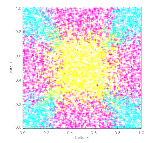
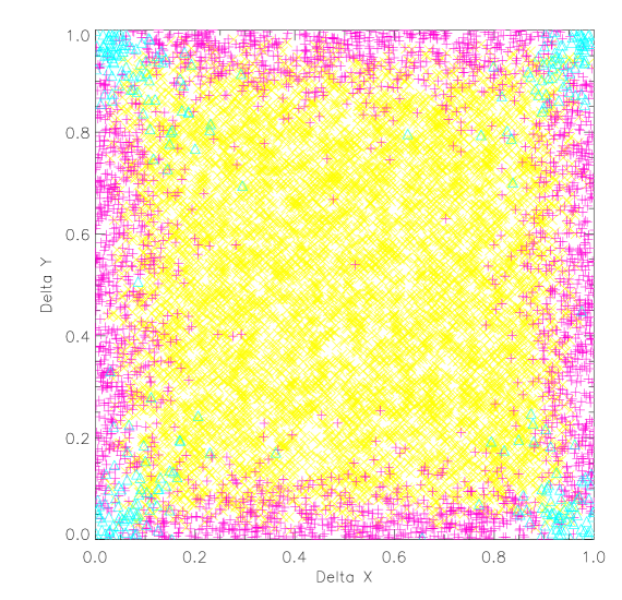
Figure 1: The photon impact positions for 3 subgroups of 13 “viable” event grades for BI (top) and FI (bottom) devices. Plus signs stand for the PIPs of 2-pixel events within a pixel, while triangles represent the PIPs of corner (3- or 4- pixel) split events. The crosses are the PIPs of single pixel events. All the photons have energy of 1.74 keV.

The first three panels in Figure 2 show the improvement in determination of PIPs enabled by the modified SER, using FI CCD simulated data at an energy of 1740 eV. For comparison, the BI simulated data of same energy photons (shown in Paper I) is included. In each panel, we show the differences between actual PIPs and repositioned PIPs from various models in chip coordinates, for all three subgroups of events. The plot axes are in ACIS pixel units, i.e., 0.5 difference represents 12 $\mu$m, and indicates photons that interacted near the pixel boundaries. The first panel from left shows the difference of actual PIPs for a random spatial distribution of events with unrandomized, standard-processed PIPs which are assumed to lie at the event pixel centers; one can see the expected uniform random distribution within the pixel. The second panel is the difference after applying TSER, in which only corner split events were repositioned. A big improvement for the small fraction of events that occur near corners can be seen. However, due to the small proportion of corner split events, there is no correction for most events. This fact is more obvious for the FI simulations. The third panel shows the difference after the static SER correction, in which the 2-pixel split events also were repositioned. For FI devices, SSER results in a “#”-shape structure, because the uncertainty of 2-pixel events can only be minimized in one direction. However, the smaller PIP differences of the SSER method relative to the Tsunemi et al. (2001) method are apparent, with the improvement more obvious for BI devices. The other two panels in the Figure will be discussed later.

Essentially, the PIP differences plotted in figure 2 represent the corrected PIP uncertainty (or probability distribution) within a pixel, and therefore can be considered as representing the ACIS pixel shape and size after SER correction. Adopting this concept, one sees that the far left panel reflects the ACIS pixel after standard CXO/ACIS processing, i.e., a square pixel with 24 $\mu$m width. After TSER and SSER correction, the effective ACIS pixel becomes smaller in size, and no longer has uniform spatial response.

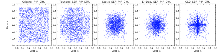
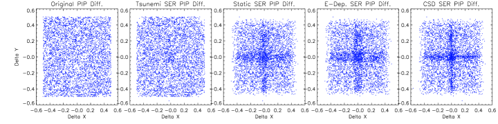
Figure 2: Differences between actual photon impact positions and processed event assumed locations for 1.74 keV events, in Chip coordinates. $1^{st}$ panel (from left): ACIS assumed PIP; $2^{nd}$ panel: correction using corner events only (Tsunemi et al. 2001); $3^{rd}$ panel: static SER correction; $4^{th}$ panel: EDSER correction; $5^{th}$ panel: CSDSER correction. The panels are in units of pixels. The top row panels are for BI devices, while the bottom row panels are for FI devices, for 4000 (BI) and 5000 (FI) photons with uniformly random landing positions.

3 Further Modifications to SER Based on ACIS CCD Simulations

3.1 Energy-dependent SER for FI CCDs

In Paper I, an energy-dependent SER method was proposed for BI devices, based on simulations for a BI CCD model. The advantages of this method were demonstrated from both simulated data and real observations. Figures 3 and 4 show the motivation for ED SER from the simulation, i.e., the branching ratio and the mean offset of the split event position, and, hence, the mean shifts for each subgroup of split events are strongly energy dependent. Therefore, adjusting assumed PIPs according to energy should significantly improve SER performance.

Figure 3 shows the percentage of events of a given split morphology as a function of photon energy, while Figure 4 shows the mean shift in position for different split event types, for FI devices. For comparison, we include the same plots for BI CCDs that were published in Paper I. Note the differences between BI and FI devices. For BI CCDs, both subgroup event percentage and mean PIP shift depends sensitively on energy, at low energy (E $<$ 2 keV). The 3 subgroups of split event percentages and PIP shifts are insensitive to energy for E $>$ 6 keV. This reflects the fact that, for photons with energy exceeding 6 keV, the characteristic penetration depth becomes comparable to or larger than the thickness of the ACIS BI CCD, which is only 45 microns. In contrast, ACIS FI CCDs are much thicker, with larger depletion depth ($\sim$ 70 $\mu$m, Prigozhin et al. 1998a). Therefore, the branching ratios and PIP shifts depend sensitively on energy over most of the CXO/ACIS bandwidth.

EDSER consists of repositioning the split event PIPs by event grade, using the mean PIP offset look-up table as a function of photon energy derived from data shown in figure 4. PIP determination benefits from applying the mean energy-dependent shifts for different split event groups. The fourth panels (from left) of Figure 2 demonstrate the PIP differences after EDSER for BI and FI devices. Compared with static SER, the EDSER BI data displays a more concentrated structure in the center, indicating the split events were relocated more accurately, and the energy dependent SER method will improve SER performance, via better PIP determination. However, due to narrower confinement of split events to pixel boundaries, one doesn’t see the same improvement for FI data in Figure 2, indicating that EDSER may not yield much gain over SSER, for FI CCDs.

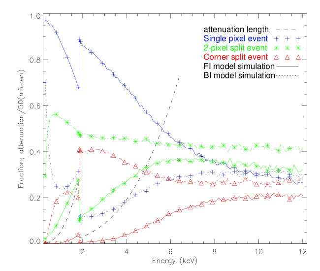
Figure 3: The fraction of different event grades versus photon energy. Results from simulations of FI (solid line) and BI (dotted line) CCD model. The X-ray attenuation length in silicon is overplotted, in units of 50 microns.

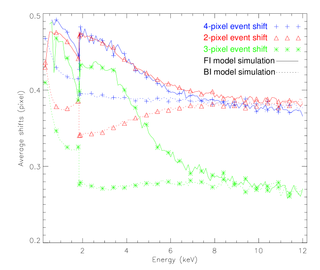
Figure 4: The mean shifts from pixel centers of the 3 subgroups of split events, according to the photon energy. FI CCD model simulations are plotted with solid line, while BI simulations with dotted line.

3.2 Charge Split Dependent SER

Simulations show that, for a split event, the proximity to the split boundary of a photon impact position is related to the proportion of the charge deposited in split pixels relative to the total charge generated by the photon. This fact provides motivation for an SER algorithm that is both energy and charge split proportion dependent. Figure 5 shows distances of PIPs (relative to split boundaries) as a function of the charge split proportion, for three types of split events. ACIS CCD models were used for these simulations, at a photon energy of 1740 eV. The simulated results are shown in the left and right columns, for BI and FI devices respectively. The measured fraction is the proportion of charge within a split pixel relative to the total charge generated by the event, including all split charge that exceeds the split threshold. For 3- and 4-pixel split events, the charge fraction in both horizontal and vertical split pixels was measured independently. The charge fraction in the diagonal split pixel of the 4-pixel split events was not measured, since the fractions from the other two split pixels already provide information about photon landing locations.

The plot shows that, with only energy information, the PIP uncertainty is relatively big since it includes all “local” uncertainties. By including charge split proportion information, one can divide the uncertainty into local uncertainties, i.e., the uncertainty at each split fraction. For example, for a 3-pixel split in BI device (the middle panel of the left column), the total uncertainty is about 0.4 pixel, while the local uncertainty at 0.4 split fraction is only about 0.03 pixel. Therefore, including charge split information, CSDSER will greatly reduce PIP uncertainties. The function describing PIP offset in terms of split charge fraction for horizontal and vertical directions is assumed indistinguishable, for a given split-event subgroups, at the same energy.

The rightmost panels in figure 2 show the simulated PIP uncertainties after CSDSER correction for BI and FI devices, at the energy of 1740 eV. The improvement in PIP determination for those panels can be seen, especially for BI devices, compared with EDSER correction. Figure 2 suggests an increasing degree of image quality improvement can be achieved, by using SSER, EDSER and CSDSER.

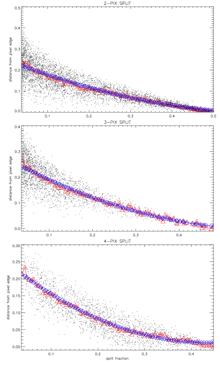
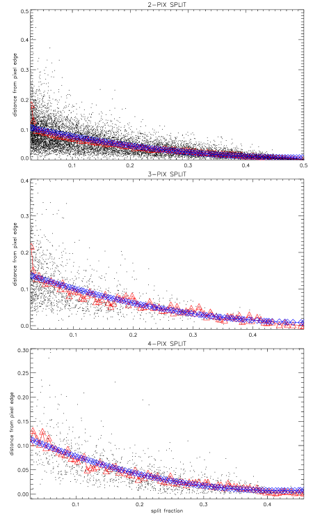
Figure 5: The distance of photon landing locations from the split boundaries as a function of charge split proportion for three split event types. The photons have energies of 1740 eV. Simulations were performed with MIT BI (left column) and FI (right column) ACIS models. The dots in the panels represent the PIP relative to split boundaries, while the red triangles are the local averages of the PIPs, and the blue lines are the polynomial regression curves of the local averages.

4 Testing SER: End-to-end Simulations

MARX (Model of AXAF Response to X-rays) is a program suite that can run in sequence to simulate Chandra on-orbit performance, with FITS file and image output (MARX technical manual). The built-in instrument models, including HRMA (High Resolution Mirror Assembly) and focal plane detectors, enable MARX to perform a ray-trace and thereby simulate Chandra CCD imaging spectroscopy of a variety of astrophysical sources. Post-processing routines can simulate aspect movement and ACIS photon pile up. However, ACIS simulations within recent versions of MARX do not include a high-fidelity CCD model. Therefore, SER related simulations must rely on CCD models (such as those described in sections 2 and 3) to analyze the CCD charge distribution and event grade formation and, therefore, SER implementation.

To test the extent to which various SER techniques should improve image performance for BI and FI CCDs, we have carried out simulations combining MARX with MIT BI/FI CCD models. We performed simulations of 50 point sources with realistic spectral distributions at positions ranging from on-axis to $160^{\prime\prime}$ off-axis, in steps of $3^{\prime\prime}.2$ (see figure 6 and 7). The MARX telescope “internal dither” model was used, with standard (default) values of 1000 and 707 second dither periods in RA and DEC directions, respectively, and an 8 arcsec dither amplitude in both directions.

The BI and FI simulation spectra are based on the averaged spectra of BI and FI ONC observations, respectively. The BI simulation spectrum was calculated from 20 point-like sources of BI ONC (obsID 4), while the FI simulation spectrum was calculated from an average spectrum of 32 well-shaped X-ray sources from a deep CXO/ACIS-I observation (see section 5). These 32 sources were also used in sections 2 and 5, for source split event branching ratios (table 1) and various SER method evaluations (figures 8 and 9), respectively. The BI and FI spectra are plotted in figure 6 and 7, respectively.

The degree of improvement due to the SER algorithms was evaluated numerically by calculating source FWHM before and after applying SER. Tsunemi et al. (2001) and Paper I give the definition of improvement; i.e., by assuming that $\mit F_{B}$ and $\mit F_{A}$ are the FWHMs of a source before and after applying SER, respectively, then the improvement $\Delta$ is defined as:

$$\Delta\,=\,\sqrt{{\mit F_{B}^{2}\,-\,F^{2}_{A}}}/F_{B}$$

The results of the simulations are shown in Figures 6 and 7 for BI and FI models, respectively. The progressively better performance of SSER , EDSER, and CSDSER is apparent in BI simulations, as expected, due to better PIP determination from addition photon and charge split information (see table 2). However, the performance of SSER, EDSER and CSDSER is very comparable in the case of FI devices, even though we might expect to see the improvement (e.g., of CSDSER relative to SSER) theoretically. In comparison to BI devices, the lack of improvement in imaging performance under the refined SER approaches for FI CCDs is most likely due to the following factors:

1. FI devices generate fewer split events than BI devices, especially corner split events. Therefore single pixel events dominate over the better repositioned split events.

2. For soft sources, such as those simulated here, the charge cloud size is relatively small. Therefore most split events in FI CCDs are very close to the split boundaries, not widespread as in BI devices. As a result, the positional uncertainties of two-pixel split events forms a long arm cross structure after applying SER. The uncertainty in the direction parallel to the split boundary is larger and remains unchanged.

3. Because of the small charge cloud, the PIP determinations of EDSER and CSDSER do not provide significant advantages over the static method, as for BI devices.

4. The slight potential improvement offered by CSDSER is degraded by telescope PSF, which includes contaminations from both HRMA PSF and aspect blurring.

Table 2: Comparison of various BI and FI SER methods.

			Degree of improvement
	Off-axis range	CCD type	CSD $>$ EDa	CSD $>$ SSERb	ED $>$ SSERc
50 sources	0—$158^{\prime\prime}.7$	BI	$68\%$	$86\%$	$80\%$
		FI	$56\%$	$52\%$	$56\%$
25 sources	0—$78^{\prime\prime}.5$	BI	$64\%$	$96\%$	$88\%$
		FI	$56\%$	$60\%$	$64\%$

Notes. —
a). Percentage of sources for which CSDSER FWHM improvement is larger than that of EDSER.
b). Percentage of sources for which CSDSER FWHM improvement is larger than that of SSER.
c). Percentage of sources for which EDSER FWHM improvement is larger than that of SSER..

Figures 6 and 7 show that SER algorithms are highly source location dependent, i.e., all SERs have better performance for on-axis sources, and the improvement decreases when off-axis angle increases. This is because the telescope PSF increases in size with off-axis angle and, therefore, the influence of the event repositioning decreases.

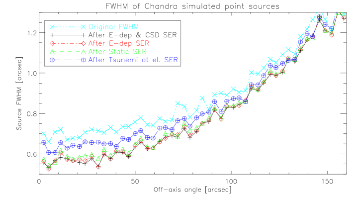
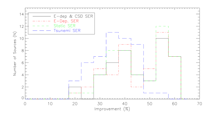
Figure 6: Improvement comparison of different BI SER algorithms, from BI CXO/ACIS point-source simulations. Top: spectrum used in the simulations (see text). Middle: improvement in source FWHM as function of source off-axis angle. Bottom: histogram of FWHM improvements.

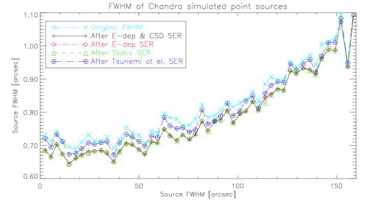
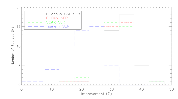
Figure 7: As in Fig. 6, improvement comparison of different FI SER algorithms from FI CXO/ACIS point-source simulations.

5 Application of the SER Algorithms to X-ray sources in Orion

The steps involved in implementing SER on real Chandra observations were discussed in paper I, and BI SER algorithms (TSER, SSER and EDSER) were evaluated from data obtained for the ONC (Orion Nebula Cluster, Schulz et al. 2001). Here we compare CSDSER with other SER algorithms for BI data (top panels in figures 8 and 9). The same implementation steps hold for FI CCDs, except the chip orientation differences within eight FI chips. Similar plots for applications of SER methods on FI Chandra Orion Ultradeep Project (COUP) data are shown in the bottom panels.

The Chandra Orion Ultradeep Project combines six consecutive observations of the Orion Nebula Cluster taken in January 2003 with the Advanced CCD Imaging Spectrometer on board the Chandra X-ray Observatory (Weisskopf et al. 2002). The total exposure time of $0.84$ Ms and over 1600 sources are detected.

COUP data reduction started with the Level 1 event files provided by the Chandra X-ray Center. Only events on the four CCDs of the ACIS I-array were considered. Event energies and grades were corrected for charge transfer inefficiency (CTI) using the procedures developed by Townsley et al. (2001 ApJL). The data were cleaned from a various potential problem events with the grade, status, and good-time intervals filters as described in the Appendix of Townsley et al. (2003). Sequences of single pixel cosmic ray afterglow events were identified but not removed from the dataset at this time. Bad pixel columns with the energies $<700$ eV and the background events with the energies $>10500$ eV were removed.

Event positions were adjusted slightly in three ways. First, individual corrections to the absolute astrometry of each of the six COUP exposures was applied based on several hundred matches between a preliminary catalog of Chandra sources and near-infrared sources in a forthcoming catalog from the ESO Very Large Telescope. Second, the sub-arcsecond broadening of the PSF produced by the Chandra X-ray Center’s pipeline randomization of positions was removed. Third, the tangent planes of five COUP exposures were re-projected to match the tangent plane of the first observation (ObsID 4395). The six exposures were then merged into the single data event file used in this paper.

5.1 Results

Based on the above steps, we have plotted the FWHM of 22 bright point-like sources in BI ONC data, obtained by Chandra/ACIS-S3. The sources were selected to represent a range in off-axis angle from $2^{\prime\prime}.72$ to $136^{\prime\prime}.8$, and in count rate from $0.0052$ to $0.2791$ s^-1 (Paper I). The top panel in figure 8 shows that after applying SER technique to these data, all SER algorithms (sec. 3) improved the FWHM for every source (except that source 1 has no improvement after applying the Tsunemi et al. [2001] method). The bottom panel displays 32 point-like sources (could be different with BI sources) chosen from Chandra/ACIS-I COUP observation, with count rate from $0.0027$ to $0.0799$ s^-1, and in off-axis angle from $0^{\prime\prime}.35$ to $125^{\prime\prime}.8$. Both abscissa axes are source number, sorted with the FWHM of original point sources, before applying SER but after removing randomization. Furthermore, COUP data process includes CTI correction (Townsley et al. 2002), to reduce charge transfer problem in ACIS-I CCDs and to recover event grade information.

The source size, represented by FWHM, was apparently smaller after applying SER approaches on BI devices, from TSER to SSER, then to EDSER and to CSDSER, as predicted by BI simulation, demonstrating the capability to improve the spatial resolution of BI Chandra/ACIS imaging. At the same time, FI devices illustrate more modest improvements, by applying SER techniques. The better performance of static SER than TSER is evident, but from SSER to EDSER and CSDSER, the improvement is less clear, for the reasons discussed in section 4. However, a small improvements in effective FI Chandra/ACIS PSF still can be seen after application of SER techniques.

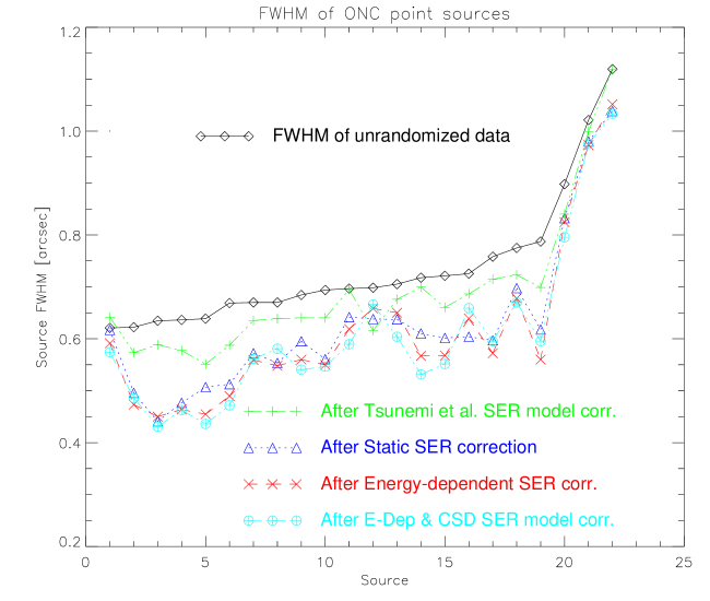
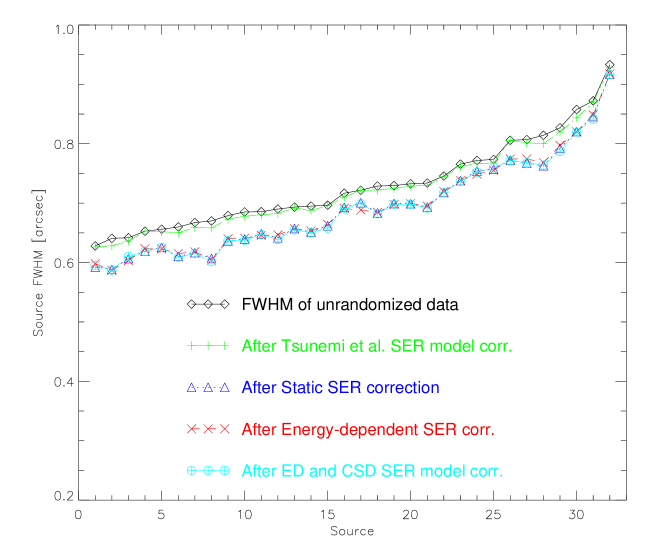
Figure 8: FWHM of BI and FI ONC point like sources before and after applying various SER algorithms described in this paper.

Using the definition of improvement given in section 4, we quantitatively evaluate the performance of different SER methods on ONC data. The top and bottom part of figure 9 shows this metric of the improvement for all SER algorithms for BI and FI Chandra/ACIS sources, respectively. As expected from MARX simulations, BI data shows superior improvement for CSDSER and EDSER, while FI data only shows improvement for modified SERs, and there is no favorite among the three modified methods. Improvement for most sources in FWHM range is from 40% to 70%, and from 20% to 50%, for BI and FI CCDs, respectively, with the improvement statistically dependent on off-axis angle.

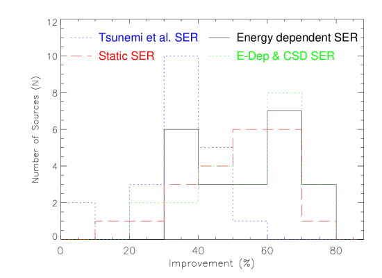
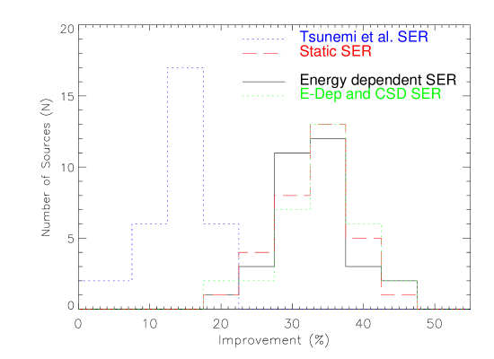
Figure 9: Comparison of image FWHM improvements using Tsunemi et al. (2001) model, static, energy-dependent SERs, ED and CSD SER on BI and FI CXO ONC data.

6 Summary

A study of potential improvements to subpixel event repositioning (SER) for CXO/ACIS data was conducted here, for BI and FI devices. We formulate modified SER algorithms at three levels of improvement for both CCD types: (1) inclusion of single-pixel events and two-pixel split events (“static” SER); (2) in addition to event grade/split morphology, accounting for the mean energy dependence of differences between apparent and actual photon impact positions, based on the results of CCD simulations (“energy-dependent” SER); (3) dependence of the actual PIPs according to the split charge proportion in the split pixel(s), event type, and event energy, based on CCD model simulation results ”charge split dependent” SER).

All three modified SER methods produce improvements in spatial resolution over those possible using a static SER algorithm employing only corner-split events (Tsunemi et al. 2001), for both BI and FI devices. BI and FI CCDs exhibit different performance and, overall, BI applications benefit more from angular resolution improvement after applying SER techniques. In addition, BI data demonstrate the superiority of energy and/or charge split dependent SER methods, while FI data show only marginal differences between the various modified SER methods.

References

- (1)
- (2) Kastner J., Li J., Vrtilek S., Gatley I., Merrill K., & Soker N. 2002, ApJ, 581, 1225
- (3)
- (4) Li J., Kastner J., Prigozhin G., & Schulz N. 2003, ApJ, 590, 586
- (5)
- (6) Mori K., Tsunemi H., Miyata E., Baluta C., Burrows D., Garmire G., & Chartas G. 2001, in ASP Conf. Ser. 251, New Century of X-ray Astronomy, ed. H. Inoue & H. Kunieda (San Francisco:APS), 576
- (7)
- (8) Prigozhin G., Bautz M., & Ricker G. 2003, Proc. SPIE 4851
- (9)
- (10) Prigozhin G., Gendreau K., Bautz M., Burke B., & Ricker G. 1998a, “The Depletion Depth of High Resistivity X-ray CCDs”, IEEE Transactions on Nuclear Science, vol.45, No.3, pp. 903-909
- (11)
- (12) Prigozhin G., Rasmussen A., Bautz M., & Ricker G. 1998b, “A model of the X-ray response of the ACIS CCD”, SPIE Proceedings, vol. 3444, pp. 267-275
- (13)
- (14) Schulz N., Canizares C., Huenemoerder D., Kastner J., Taylor S., & Bergstrom E. 2001, ApJ, 549, 441
- (15)
- (16) Townsley L., Broos P., Nousek J., & Garmire G. 2002, NIM-A 486, 751
- (17)
- (18) Townsley L., Feigelson E., Montmerle T., Broos P., Chu Y., & Garmire G. 2003, ApJ, 593, 874T
- (19)
- (20) Tsunemi H., Mori K., Miyata E., Baluta C., Burrows D.N., Garmire G.P., & Chartas G. 2001, ApJ, 554, 496
- (21)
- (22) Weisskopf M., Brinkman B., Canizares C., Garmire G., Murray S., & Van Speybroeck L. 2002, PASP, v114, 791