A Strategy for Finding Near Earth Objects with the SDSS Telescope

Abstract

We present a detailed observational strategy for finding Near Earth Objects (NEOs) with the Sloan Digital Sky Survey (SDSS) telescope. We investigate strategies in normal, unbinned mode as well as binning the CCDs 2$\times$2 or 3$\times$3, which affects the sky coverage rate and the limiting apparent magnitude. We present results from 1 month, 3 year and 10 year simulations of such surveys. For each cadence and binning mode, we evaluate the possibility of achieving the Spaceguard goal of detecting 90% of 1 km NEOs (absolute magnitude H $\leq$ 18 for an albedo of 0.1). We find that an unbinned survey is most effective at detecting H $\leq$ 20 NEOs in our sample. However, a 3$\times$3 binned survey reaches the Spaceguard Goal after only seven years of operation. As the proposed large survey telescopes (PanStarss; LSST) are at least 5-10 years from operation, an SDSS NEO survey could make a significant contribution to the detection and photometric characterization of the NEO population.

key words: solar system: general — minor planets, asteroids — surveys

1. Introduction

Collisions with Near Earth Objects (NEOs) pose a devastating threat to the safety of the Earth. (An NEO is an asteroid or comet with perihelion distance $q\leq$ 1.3 AU and aphelion distance $Q\geq$ 0.983 AU.) Current estimates of the global impact threat suggest that a collision with an object of 1 km diameter is likely to cause global disaster in the form of massive loss of food crops and tsunami-generated flooding, while larger asteroid (10 km) impacts would likely result in near-global extinction of the majority of advanced life forms (Morrison, Spaceguard Survey report, 1992). Discovering and characterizing large NEOs is therefore a high priority from a hazard viewpoint. To address this hazard, Congress and NASA developed the Spaceguard goal, first stated in 1995 and implemented in 1998, to discover 90% of NEOs larger than 1 km in diameter within ten years (Shoemaker, NEO Survey Workgroup report, 1995). The Sloan Digital Sky Survey (SDSS) 2.5m telescope and camera system (York et al. 2000) are uniquely positioned to contribute to this initiative, with an ecliptic imaging survey that is complementary to current NEO programs.

Operating in “drift scan (time delay and integrate)” mode, SDSS has been shown to be very effective at detecting and characterizing Solar System objects (Ivezić et al. 2001, 2002; Jurić et al. 2002) using the movement of the objects between the five filters in a single scan to discriminate them from the stationary background. Most of the asteroids observed in this way are new detections, because moving objects can be found over a wider field at fainter magnitudes than the completeness limits of currently available asteroid catalogs. However, the main survey strategy results in only one imaging scan for a given region of sky, and therefore orbits have not been obtained for these objects.

Matching the SDSS moving objects catalog against asteroids with known orbits has demonstrated that asteroid colors in the SDSS passbands are tightly correlated with orbital parameters (Ivezić et al. 2002). This work has contributed significantly to the study of asteroid families, which are thought to be the remnants of disrupted larger bodies, and therefore to the study of the origin of the Solar System. The asteroid colors are also important for assessing the impact hazard, as there is a factor of 4 difference in the albedos of different asteroid taxonomic classes, and the uncertainty in albedo translates directly into an uncertainty in size and therefore potential hazard. SDSS multicolor photometry will greatly improve our ability to classify asteroids and to determine their spectral reflectivity. While other NEO projects have restricted themselves to a single wide-band filter or no filter at all, the SDSS system produces excellent photometry in 5 colors.

Jedicke et al (2003) simulated the discovery of NEOs as a function of time, in order to assess the current prospects for reaching the Spaceguard Goal of identifying 90% of NEOs larger than 1 km by 2008. They assume an observing cadence typical of LINEAR (LIncoln Near Earth Asteroid Research – the most prolific NEO survey that is currently operational), and account for actual observing conditions by assuming only nighttime observing, avoiding bright time and avoiding the Galactic Plane. They find that the LINEAR survey cannot meet the Spaceguard goal. Proposed surveys with limiting magnitudes $\sim$ 24 (LSST, Pan-Starrs) are not likely to be operational for 5-10 years. The only prospect for achieving the Spaceguard goal is therefore a dedicated survey in the V=21.5 magnitude range. As we will show in the following sections, the V=21.5 simulation corresponds closely to an NEO survey using the SDSS 2.5m telescope and imaging system.

In this paper, we simulate the detection of NEOs with the SDSS telescope using a detailed cadence and observing strategy, which attempts to maximize the detection and orbital characterization of NEOs. We place the results of these simulations in the context of the predictions of Jedicke et al. (2003) to assess the possible contribution of an SDSS NEO survey toward achieving the Spaceguard goal. We also perform 10 year simulations of NEO detection to evaluate in more detail the potential of an SDSS NEO survey.

2. The SDSS camera and telescope

The SDSS camera system (Gunn et al. 1998) consists of six columns of five photometric CCDs, with a CCD for each of the five SDSS filters (u, g, r, i, z) in each column. The system is designed to image the sky by driftscanning along great circles. In this mode, the telescope is driven in three axes so that the sky moves past the field of view along one dimension of the CCDs. The camera shifts the accumulating image along the same dimension at the same rate, and the data is read out when it reaches the edge of each CCD. In this way, a continuous image is built up in the scan direction.

The field of view of the camera is 2.5 degrees, each column of CCDs being 13.5 arc minutes wide. Two interleaved scans cover a given area completely, with 10% overlap. The apparent magnitude limits for which the SDSS system is 50% complete are 22.5 (u filter), 23.2 (g), 22.6 (r), 21.9 (i) and 20.8 (z).

Normally the SDSS driftscans at the sidereal rate, so that an object is first detected by the r filter, and subsequently by the i, u, z and g filters at intervals of 72 seconds. Moving objects can be detected by their apparent motion during the 5 minute time baseline between the r and g filters, as demonstrated in Ivezić et al. (2001), who detected moving objects with apparent motion between 0.025 and 1 degrees per day. Most asteroids are detected in the g, r and i filters.

The SDSS telescope and camera can be used to driftscan faster than the sidereal rate. The camera has a minimum readout time per pixel very close to sidereal, set by the design of the CCD controller and the charge transfer characteristics of the detectors themselves. Therefore, faster scanning is done by binning the CCDs, thereby reducing the readout time of the detectors. In order to avoid smearing the images, the rate at which the image of a star moves across the CCDs must be equal to the readout rate of the CCDs. The CCD readout time does not scale linearly with the binning: in 2$\times$2 binned mode the minimum readout time is one third of its unbinned value, and in 3$\times$3 binned mode it is roughly one fourth. Therefore, in 2$\times$2 binned mode, the telescope can cover three times as much area as in unbinned mode. The apparent magnitude limit decreases by roughly one magnitude to 22.1 (g), 21.6 (r) and 21.0 (i). The limits on apparent motion scale roughly with the scan rate (modulo the astrometric precision, which also varies with scan rate), and are roughly 0.1 – 1.5 deg day^-1 in 2$\times$2 binned mode.

Note that the magnitude limits given are 5$\sigma$ detections (S/N $\geq$ 5). More relevant to the detection of moving objects is the apparent magnitude for which some fraction of moving objects is detected. Jedicke et al. (2003) define V_50%, the V magnitude for which 50% of moving objects are detected. Ivezić et al. (2001) and Jurić et al. (2002) demonstrated that $\sim$ 90% of moving objects are detected in unbinned mode to 21.5 magnitudes in r. The main difficulty in detecting fainter moving objects is the large number of false positives. We propose to detect $>$50% of moving objects to the 5$\sigma$ magnitude limit. It should be much easier to remove false positives with a dedicated survey such as we are proposing, because any given patch of sky will be observed multiple times.

3. NEO Model Population

Our simulations are based on the theoretical NEO population of Bottke et al (2002). Their model assumes that the NEO population is in a steady state, being populated by small bodies from five source regions: (i) the $\nu_{6}$ secular resonance in the main asteroid belt (37% $\pm$ 8%), (ii) the 3:1 Jupiter mean motion resonance at 2.5 AU (25% $\pm$ 3%), (iii) the Intermediate Mars Crossing region (23% $\pm$ 8%), (iv) the outer main asteroid belt (8% $\pm$ 1%), and (v) Jupiter Family Comets (JFCs) (6% $\pm$ 4%), low-inclination comets with origins in the Kuiper Belt (Levison & Duncan, 1997). The only population of solar system objects not included in this model which poses a threat to the Earth are the Nearly Isotropic Comets (NICs), which originate in the Oort Cloud and make infrequent passages to the inner solar system.

The sample distribution we used (obtained from W. Bottke, private communication) contains 4668 NEOs with absolute magnitude H $\leq$ 20 (diameter D $\geq$ 400m assuming an albedo of 0.1), including 961 NEOs larger than 1 km (H $<$ 18). The population has orbital eccentricities centered near e=0.6, orbital inclinations peaking near 10-20 degrees but with a significant tail to higher inclination, and semimajor axes ranging from 0.5 AU to past 4 AU with a broad peak near 2 AU. The distributions of the NEO model population in each of these parameters are shown with the black lines in Figure 1. The red lines indicate the distributions of the currently known NEO population (from the Minor Planet Center database, as of May, 2003).

It is clear from Figure 1 that a significant number of asteroids with d $>$ 1 km remain to be found.

4. Simulation Parameters

We use the Bottke NEO model as an underlying population, and sample it using the SDSS imaging system at various binning, cadence, position, etc. to optimize the number of NEO detections that lead to orbital solutions. The simulations are guided by the following information:

Weather: Weather statistics for Apache Point Observatory (APO) were compiled from two sources. Data from the Astronomy Research Consortium (ARC) 3.5m telescope averaged over several years show that approximately 35% of the available observing time is lost to weather, 15% of the time is photometric, and 50% is “spectroscopic”, i.e. the dome is open and data are being obtained, but the conditions are not photometric. SDSS spectroscopic observing logs, scaled to include bright time, indicate that $\sim$ 45% of the available time is used for spectroscopy. This NEO survey was intended to be conducted in parallel with other science programs requiring photometric conditions. We therefore adopt the “spectroscopic” time for our simulations. This amounts to an average of 15 nights per month. If this survey were the sole program using the SDSS telescope, it would average 19-20 usable nights per month, and would improve the results in the upcoming sections.

Ecliptic Latitude: Figure 2 (top panel) shows that the Bottke model is roughly approximated by a Gaussian distribution with a FWHM of about 10 degrees. The bright, nearby, “detectable” population (r $<$ 21.5) has a broader distribution, similar to a Gaussian with a FWHM of about 20 degrees. This suggests that an NEO survey should not concentrate entirely on the ecliptic equator, but should extend in latitude on each side of the equator. However, the marginal gains decrease at latitudes past $\pm$20-30^∘. Note that at any given time, roughly 1000 of the 4668 NEOs in our sample are detectable. Thus, any survey must operate for several years in order to detect a sizeable fraction of NEOs, with a survey length that correlates inversely with limiting magnitude. Note that survey length does not scale linearly with detectability, as it takes far longer to detect the second 50% of an NEO population than the first 50%. We return to this issue in sections 7 and 8.

Solar Elongation: Figure 2 (bottom panel) plots the detectability of NEOs as a function of solar elongation in the ecliptic plane (i.e. geocentric ecliptic longitude at zero geocentric latitude, as measured on March 21). A solar elongation of 180 degrees corresponds to opposition, while 0 (and 360) degrees is the position of the Sun. Competing effects conspire to give the three peaks in the diagram. Objects at opposition are completely illuminated by the Sun, and therefore have brighter apparent magnitudes, and also have observable velocities favorable for detection. However, the volume inhabited by the NEO population which is encompassed within the solid angle of the detector is a minimum at opposition, which reduces the density of objects on the sky.

The peaks at solar elongations of roughly $\pm$ 60 degrees (i.e. near 60 degrees and 300 degrees; called the “sweet spots”) also result from competing effects. The density of NEOs on the sky is highest in the direction of the Sun, as most NEOs are farther away from the Earth, and a larger volume is being sampled in that direction than away from the Sun, at opposition. However, observing within about 45 degrees of the Sun is very difficult, especially for ground-based telescopes. NEOs which lie between the Earth and Sun will show large phases, and therefore be faint. The holes in the distribution near elongations of 120 and 240 degrees are the places in the orbits where the velocities are not favorable for detection (i.e. the apparent velocities drop below 0.1 deg day^-1). The sweet spots arise as a balance between these effects, and are a prime location for detecting and characterizing NEOs.

The above reasoning argues for an observing strategy that targets specific solar elongations on a given night, that is breaking the night up into several short scans – see Figure 4 – rather than obtaining a single scan that covers the entire observable ecliptic plane.

5. Observing Strategy

We investigated unbinned (1$\times$1), binned (2$\times$2) and binned (3$\times$3) scans, extending to $\pm$10-40 degrees in ecliptic latitude, and with various ecliptic longitude sampling. Our results are as follows:

Binned vs. Unbinned: As mentioned above, unbinned observations scan the sky at the sidereal rate, 2$\times$2 binned observations scan the sky three times faster, and 3$\times$3 binned observations four times faster. The approximate limiting magnitudes for unbinned, 2$\times$2 and 3$\times$3 binned scans in the r band are 22.5, 21.5 and 21.1, respectively. The limits on apparent velocity are determined by the time between exposures in the r and g filters, and are roughly 0.025-1 deg day^-1, 0.1-3 deg day^-1 and 0.15 - 4 deg day^-1 for the three cases. This trade-off between sky coverage and depth of coverage is investigated in the upcoming sections.

Calculation of Observables: We used the JPL “Horizons” program (Giorgini et al 1996) to generate ephemerides for each object in our NEO population each night for a period of three years. From our knowledge of the position of each object in space we calculate the relevant parameters: phase angle, solar elongation, heliocentric and geocentric distances. We calculate the size distribution of NEOs, assuming all NEOs have an albedo of 0.1. The apparent magnitude is calculated following the method of Bowell et al (1989), assuming a slope parameter G of 0.23, which is typical for S type asteroids, and a reasonable, albeit slightly higher than average, value for NEOs (Morbidelli et al 2002). The result of these calculations is a (large) data table that gives us all the observable quantities for each NEO in the population at each time throughout the three year simulation.

Orbits: Previous efforts (Bowell et al. 2002) indicate that 3-4 observations spaced over a few up to 20 days will provide a good fit to a typical NEO orbit. To test our ability to recover orbits, we use the output of a given month of simulation as input to an orbit finding program (ORBFIT- Milani 1999). We used the detections on both the g and r chips (hence an instantaneous velocity vector) in the orbit fitting. Figure 3 shows that orbits are recovered at the 65-70% level if three observations are available, and that the spacing of the three observations is not critical for any of the individual parameters. As this represents only one of a number of methods for determining orbits, we consider this value to be a lower limit on the fraction of orbits accurately obtained.

This requirement for orbital determination, together with the weather statistics, constrains the frequency and number of revisits to a given field, and therefore the cadence.

Auxiliary Data: The possibility of obtaining auxiliary followup data on other telescopes would greatly increase the number of objects found with good orbits, allowing translation along the green curves in Figure 1 from the dotted line (1 detection) to the dashed line (2 detections) to the solid line (3 detections, and well determined orbit), giving roughly a factor of two increase in NEOs with orbits over those that could be found using the SDSS system alone. We note that detection of the objects is the primary requirement, and possible systematic differences in photometric calibration are not a major concern.

Cadence: In order to maximize the number of NEOs for which accurate orbits are determined, we devised a strategy whereby we observe two contiguous (in latitude) stripes (each stripe consists of two interleaved strips) on alternating nights until both have been observed three times. We then offset in latitude and observe two new stripes, again alternating. Experience with the simulations suggests that approximately 5-6 stripes can be observed in a given month. We find that since most of the ecliptic longitude imaged in a given month is still available in the following month (basically the opposition and eastern peaks in the solar elongation plot, Figure 2, are still available), we can increase the total area observed by adopting a bi-monthly strategy, with one month investigating latitudes north of the ecliptic, and the next month south. This strategy balances the competing requirements to obtain several (of order 3) observations of each object and to cover as much area as possible. Figure 4 is a representation of the first three stripes in the northern direction. Note that, although the stripes are shown as scans parallel to the ecliptic equator, these are great circles on the sky, so there is a slight curvature that is not depicted on the plot.

Airmass Constraints: The SDSS telescope is located at Apache Point Observatory (APO) in New Mexico, at a latitude of 32.8^∘ North. The minimum zenith angle of the ecliptic at local midnight therefore oscillates between 9.3^∘ on the (northern) winter solstice and 57.3^∘ on the summer solstice. An optimized NEO survey may want to avoid observations at airmasses larger than 2 (zenith angles $>$ 60^∘). In that case, we would not want to observe south of the ecliptic in the summer months. A strategy could be devised whereby scans on consecutive summer months would focus solely on northern ecliptic latitudes. Alternatively, the ecliptic latitude about which monthly scans are centered could shift to 10-20 degrees north during the summer months. This issue has not been addressed to date in our cadence, but the effect on the realism of our simulations is not large, particularly since the length of the observable night is at a minimum when the ecliptic is most difficult to observe, in the summer.

6. Results

Figures 5 and 6 show the results of a 1 month simulation, using the cadence from Figure 4, binned 2$\times$2. The assumed 15 observable nights are randomly spread throughout the month, and we assume 8 hours of observing per night . To account for the presence of the Moon, the apparent magnitude limit varies sinusoidally with a 28 day period between r magnitudes of 20.5 and 21.5, which are conservative 5$\sigma$ detection limits for the binned data (see Section 2). In this particular simulation, the 147 objects were detected at least once. The orbits of 58 NEOs were determined according to the criterion of Bowell (3 observations in 10 days), and 102 objects were detected at least twice. Single and double observations can be submitted to the Minor Planet Center for followup, and are valuable to the community and the Spaceguard effort even without precise orbital elements. However, note that few current NEO surveys are as sensitive as SDSS, so this survey would be largely responsible for its own followup observations.

Our cadence is designed to observe each NEO 2-3 times, but $\sim$ 1/3 of the total detected objects are seen only once. There are two ways in which an NEO can elude multiple detection. If it is very close to the Earth, and therefore moving very rapidly on the sky with a significant component of its velocity perpendicular to the ecliptic, it will not be picked up on successive scans of the same area. In addition, the apparent magnitude of NEOs in certain orbits can change by a significant amount within a few days, through changes in their apparent phases and distances from Earth.

Our 1 month scans are extended into a year-long strategy by alternating excursions in latitude North and South of the ecliptic. This cadence detects 10-20% more NEOs in a 3 year simulation than one which scans the same area each month, including roughly twice as many H $\leq$ 18 NEOs, the targets of the Spaceguard Goal.

We have run 3 year simulations using a variety of detailed cadences (i.e. the ordering of scans A, B, C, etc. from Figure 4). Figures 7 and 8 show the results of a 3 year simulation operating in 2$\times$2 binned mode, in which 1931 NEOs were detected at least once and 1552 at least twice. Accurate orbits were derived for 994 objects. Figure 7 demonstrates that the detection volume of NEOs is a function of the NEO size. Figure 8 shows the fraction of NEOs which are detected in a given field of view, thereby quantifying the fraction of the detection volume accessible for different-sized NEOs.

Table 1 shows a comparison between unbinned, 2$\times$2 binned and two 3$\times$3 binned simulations. Each simulation lasted three years, assumed 15 nights per month of observing, and 8 hours per night. In 1$\times$1 (unbinned) mode, 120 degrees of the ecliptic are scanned in a night, divided into three pieces: scans along the two sweet spots and opposition. The scans cannot be interleaved in the same night, so it takes two full nights to cover a 2.5^∘ wide stripe on the ecliptic, thereby limiting the range in ecliptic latitude that can be covered. In 2$\times$2 binned mode, the increase in scan rate means that two scans can be interleaved, each consisting of three similar pieces which focus on the sweet spots and opposition, as shown in figure 4. In 3$\times$3 binned mode, 480 degrees of the ecliptic are scanned in a night. We have simulated two different cadences in 3$\times$3 mode: (i) increasing the length of scans to be nearly continuous in ecliptic longitude, keeping roughly the same latitude coverage as in 2$\times$2 binned mode, and (ii) concentrating on the sweet spots and opposition, and increasing coverage in ecliptic latitude. Case (ii) produced more NEO detections, as shown in table 1.

All three modes of operation result in roughly the same number of 1 km NEOs detected. Unbinned mode is the most proficient at single detections, although a large number of these are smaller objects. 2$\times$2 binned mode is the best at characterizing the orbits of NEOs, although only slightly better than 3$\times$3(ii) mode, which detects slightly more 1 km NEOs. Although a vigorous followup program could attempt to re-observe the singly and doubly detected NEOs, 2$\times$2 binned mode is the most efficient at self-followup, whereas unbinned mode produces good orbits for only about one third of the NEOs it detects.

7. Comparison with Jedicke et al. (2003) results

As of May 2003, only 1405 NEOs with H $\leq$ 20 (d $\geq$ 400m assuming an albedo of 0.1) have been discovered (out of 2307 total NEOs discovered). In 3 years, our NEO simulations show that an SDSS NEO survey could come close to matching that number for objects with well-determined orbits. However, this number does not account for the fraction of known NEOs rediscovered by SDSS.

A detailed analysis by Jedicke et al (2003) demonstrated that a deep survey with a limiting magnitude of V $\sim$ 21.5 (similar to SDSS) would reach the Spaceguard goal 10-20 years faster than the current leading NEO survey, LINEAR, which has a limiting magnitude of V_50% $\sim$ 19. The Jedicke simulations assume a cadence which covers the entire observable sky each month, which is not directly comparable to our 2$\times$2 binned strategy that surveys only to ecliptic latitudes about $\pm$ 15 degrees.

Operating in 3$\times$3 binned mode, SDSS has a limiting magnitude in the r band of 21.1, which corresponds to V $\sim$ 21.4. The sky coverage rate is four times the sidereal rate, 60 degrees per hour. Assuming 8 hours of observing per night, SDSS covers 480 degrees of ecliptic longitude in a given night. To cover a given 2.5 degree-wide “stripe”, two “strips” must be interleaved. Therefore, SDSS can cover a 2.5${}^{\circ}\times$240^∘ patch each night. In 16-17 nights, SDSS can cover 10,000 deg² of sky, roughly one quarter of the entire sky. As the latitude distribution of NEOs is not uniform (see figure 2), a search program similar to the one described above could cover the ecliptic to roughly $\pm$ 20^∘ in ecliptic latitude each month, a region in which $\gtrsim$ 80% of NEOs are found. Alternatively, a two month strategy could reach ecliptic latitudes of $\pm$ 40^∘, and $\gtrsim$ 95% of NEOs. This implies that SDSS, operating in 3$\times$3 binned mode, would be roughly equivalent to a V_50% = 21.5 survey from Jedicke et al. (2003), and would be able to detect 90% of NEOs larger than 1 km by about the year 2010 if such a program were implemented starting in 2002. However, this is a very indirect argument. In the following section we present the simulated results of 10 year NEO surveys which include a realistic pre-detected population.

8. Long-Term Simulations

To better evaluate the performance of an SDSS NEO survey, we have performed long-term, 10 year simulations of NEO discovery using the different modes of operation discussed in the previous sections. We have included a realistic pre-detected population of NEOs by running a “pseudo-LINEAR” simulation of NEO detection as in Jedicke et al. (2003) on our sample of 4668 NEOs with H $\leq$ 20. The pre-detection simulation was run until it matched the 628 NEOs with H $\leq$ 18 known as of Jan 1, 2003. At the end of this simulation the total number of pre-detected NEOs was 1424, slightly more than the 1333 H $\leq$ 20 NEOs known as of 1/1/2003 (data from the Minor Planet Center). The distributions of the known and pre-detected populations are shown in Fig 9 and match up remarkably well, giving us confidence that our pre-detected population is realistic.

The results of four 10 year simulations are shown in Figures 10 and 11, including NEOs with 2 or more detections in a span of 10 days. An unbinned survey, described in Sections 5 and 6, detects the most NEOs in 10 years. The completeness of the pre-detected population is 30%, and reaches 62% after a 10 year survey in unbinned mode. Completenesses are calculated assuming the Bottke et al. (2003) model as an underlying NEO population, as described in Section 3.

If the goal of an NEO survey is to achieve the Spaceguard goal of detecting 90% of NEOs with H $\leq$ 18, then Figure 11 shows that the 3$\times$3(ii) binned survey, described in Sections 5 and 6, is most effective. The completeness of the pre-detected population is 60%, and reaches 91% by the end of a 10 year survey in 3$\times$3(ii) binned mode. The 90% mark is reached after seven years, in January 2010. Note that this is almost exactly the time predicted by Jedicke et al. (2003) for a survey with limiting magnitude of V${50\%}$ = 21.5, and determined independently.

It is interesting that the optimal survey strategy depends on the goal of the survey. The balance between magnitude limit and sky coverage is such that a 3$\times$3(ii) binned survey is able to achieve the Spaceguard goal the fastest, while an unbinned survey detects a significantly larger fraction of the total NEO population. A 2$\times$2 binned survey does moderately well in both regimes, detecting a total of 89.3% of NEOs after 10 years.

One can imagine a long-term NEO survey which begins operation in 3$\times$3(ii) binned mode, and transitions to unbinned mode after the completion of the Spaceguard goal. Such a hybrid survey would provide the appropriate balance between survey depth and sky coverage, and adapt to the current scientific need.

9. Conclusions

The detection of km-sized potentially hazardous asteroids is a high priority. We have demonstrated that the SDSS telescope and camera system has the ability to detect and characterize the orbits of NEOs at a fast rate. We have detailed four different cadences, which depend on the binning of the CCDs, the spatial distribution of NEOs, and observational restrictions.

In 3$\times$3 binned mode, the 5$\sigma$ detection limit corresponds to V $\sim$ 21.4. The 3$\times$3 areal coverage rate implies that an SDSS NEO survey in that mode would be roughly equivalent to a V_50% = 21.5 NEO survey from Jedicke et al (2003). Their results, in turn, imply that such a survey could reach the Spaceguard goal of detecting 90% of NEOs with H $\leq$ 18 by the year 2010, had such a survey begun in early 2002.

We have performed long term, 10 year simulations of SDSS NEO surveys with each of our four cadences. We find that an unbinned survey detects the largest number of NEOs, 62% of NEOs with H $\leq$ 20 in 10 years. Alternatively, the 3$\times$3(ii) binned survey reaches the Spaceguard Goal most quickly, in 2010 for a survey beginning in January, 2003. This is very close to the prediction of Jedicke et al. (2003).

The accurate, five-band photometry of the SDSS system would also be a huge benefit to NEO science, through the composition and albedo (and therefore potential hazard) determination of NEOs. A large side benefit to Solar System science would be the serendipitous discovery and compositional determination of a large number of small solar system bodies, main belt asteroids and Kuiper belt objects. An unbinned survey would be most beneficial in this regard, due to its deeper exposures and frequent scanning of the ecliptic.

10. Acknowledgments

We gratefully acknowledge extensive discussions with our colleagues in the SDSS/APO community. Our thanks to the SDSS Advisory Council and Management Committee for supporting this effort to investigate an NEO survey, to Bill Bottke for generating our NEO sample population, and to Ted Bowell and Al Harris for helpful discussions. CH thanks NSF grant AST-0098557 at the University of Washington for support. SR and TQ are grateful to the NASA Astrobiology Institute for support.

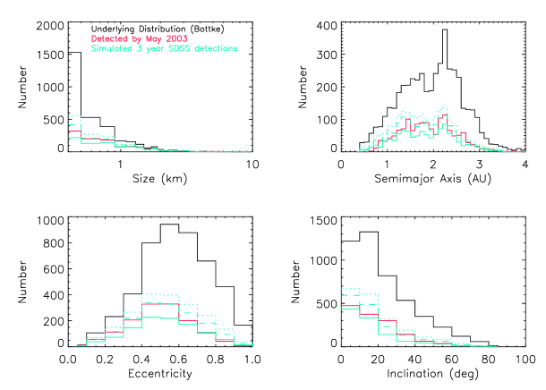
Figure 1.— The orbital parameter and size distributions of NEOs with H $\leq$ 20. The red line indicates known NEOs as of May 2003. The black line is the Bottke et al (2002) model, which we take as the underlying distribution. The number of currently known NEOs in this absolute magnitude range is 1405, where the Bottke model predicts 4668, including 961 larger than 1 km. The green lines are the NEOs detected by a 3 year simulation using our NEO strategy with the SDSS system. The dotted green line indicates NEOs detected once in our simulation (1933 objects), the dashed line indicates NEOs with multiple detections (1533 objects), and the solid green line indicates NEOs for which accurate orbits may be determined (3 detections in 10 days; 1023 objects) using only the 2.5m data. A followup program using the 3.5m and/or one of the smaller APO telescopes could provide orbits for the remaining NEOs that were detected only once or twice. Note that our model includes objects as small as 400 m, but the top left panel begins at 600 m to avoid overshadowing $\geq$ 1 km NEOs.

Figure 2.— The instantaneous distribution of NEOs from the Bottke et al (2003) model, as a function of geocentric ecliptic latitude (top) and longitude (bottom). The bottom panel shows the increased detectability of the NEO population at the sweet spots and opposition. See text for details.

Figure 3.— Results of fitting orbits with various sample cadences are illustrated. The cadences are:    2a = days 1 and 2    2b = 1,3    3a = 1,3,10    3b = 1,5,10    3c = 1,10,20    3d = 1,15,30    30a = all 30 days. The histograms show the fraction of objects in a one month simulation whose primary orbital parameters (eccentricity, semi-major axis, inclination, and the combination of all three of these parameters) can be reproduced within 1% of the input values, for each of these cadences.

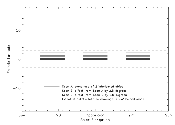
Figure 4.— Our NEO cadence for 2$\times$2 binning mode, focusing on the sweet spots and opposition. Each night consists of six 60-degree scans ($\pm$ 1.25 hours each), to fill a stripe (e.g. A). We observe the same stripe on consecutive nights, and shift in ecliptic latitude after a given stripe has been observed 3 times. Starting on the ecliptic, we shift to northern and southern latitudes in consecutive months, then repeat. A cadence for the 15 observing nights in one month is A, A, B, B, A, B, C, C, D, D, C, D, E, E, F, where each lettered stripe is offset from the previous one by 2.5 degrees. Stripes A, B and C are illustrated in the figure (not to scale). The stripes are great circles and will exhibit slight curvature in this coordinate system (not shown).

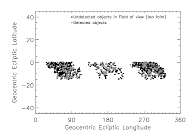
Figure 5.— The top panel shows detections (grey dots) in a 1 month simulation as a function of ecliptic latitude and geocentric ecliptic longitude. The month of March was used, so that opposition corresponds to longitude of 180 degrees at the vernal equinox. The black dots indicate objects which fell inside the camera’s field of view, but were too faint for a 5$\sigma$ detection. The parallelogram shape results from the movement of opposition and the sweet spots in the ecliptic coordinate system by 30 degrees through the month. The histogram on the bottom is made up solely of the detected objects, and shows the sweet spots expected from Figure 2.

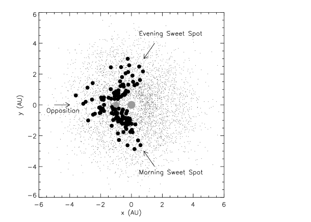
Figure 6.— Detections in the 1 month simulation from Figure 5, in x-y coordinates. The Sun is depicted in grey at the origin, and the Earth in grey at the appropriate location in its orbit and a distance of 1 AU. The large dots represent NEO detections, and the small dots represent the total instantaneous distribution of NEOs. The sweet spots and opposition are labeled, with the “evening sweet spot” being observed first after sunset.

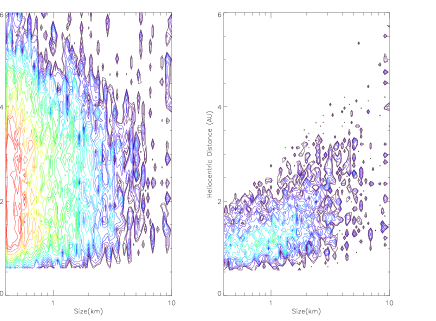
Figure 7.— The detection volume of NEOs in apparent magnitude - diameter space. The left panel shows the underlying distribution of detectable NEOs in a 3 year simulation, while the right panel shows the ones detected with our proposed 3 year NEO survey operating in 2$\times$2 binned mode. The fraction of detected objects increases with size, as their detection volume increases. The detection volume is a function of the size, albedo, and phase of an asteroid. Our distribution assumes an albedo of 0.1 for all objects. The contours are logarithmically spaced for clarity.

Figure 8.— The fraction of NEOs in our field of view which were detected as a function of size for the same 3 year simulation as in Figure 7. It is clearly much easier to detect larger objects which have correspondingly larger detection volumes. Note that, of our sample of 4668 NEOs, 961 are larger than 1 km (assuming an albedo of 0.1) , and the number of objects per bin is small past five km.

Figure 9.— A comparison between our pre-detected population (dashed lines) and the population of known NEOs (solid lines) as of Jan 1, 2003. The agreement between the samples indicates that this is a realistic representation of the known NEO population.

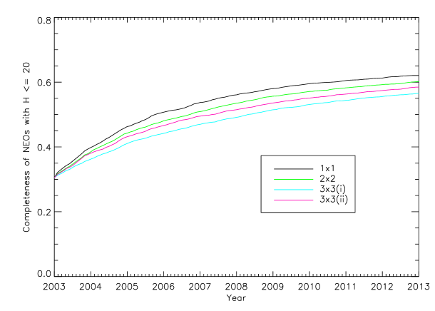
Figure 10.— Completeness of all NEOs with H $\leq$ 20 in our sample as a function of time, including the pre-detected population from Figure 9, labeled as in Table 1. An NEO survey in unbinned (1$\times$1) mode is the most efficient. A 10 year unbinned survey increases the completeness of H $\leq$ 20 NEOs from 30% to 62%.

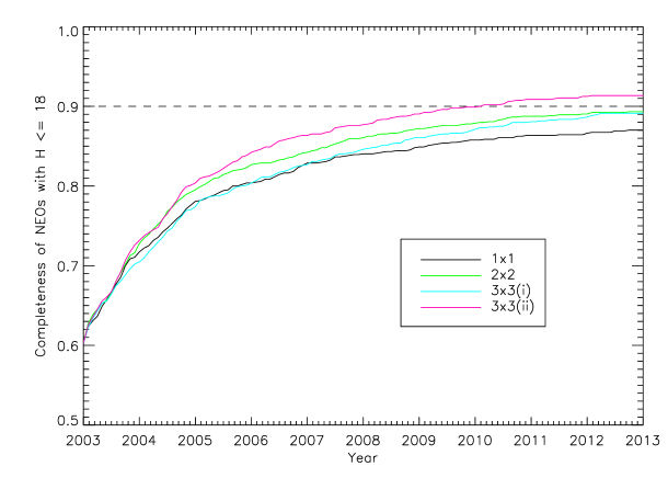
Figure 11.— Completeness of NEOs with H $\leq$ 18 (d $\geq$ 1 km for an albedo of 0.1) as a function of time, labeled as in the previous figure. The dashed line represents a completeness of 90%. A survey in 3$\times$3(ii) binned mode detects larger NEOs the fastest, in contrast with the previous figure which shows that an unbinned survey has the highest detection rate for all NEOs with H $\leq$ 20. A 3$\times$3(ii) binned survey could have achieved the Spaceguard goal of detecting 90% of H $\leq$ 18 NEOs by early 2010, had it begun in January 2003.

Table 1Results of 3-year NEO Simulations

	1$\times$1	2$\times$2	3$\times$3(i)	3$\times$3(ii)
Limiting r magnitude	22.5	21.5	21.1	21.1
Ecliptic Latitude Coverage	$\pm$10∘	$\pm$15∘	$\pm$20∘	$\pm$30∘
NEOs with 1+ detections	2184	1929	1671	1781
NEOs with 2+ detections	1641	1533	1341	1439
NEOs with orbits	699	1023	566	991
NEOs ($>$ 1 km)	756	758	735	774

References

- (1)
- (2) Bottke, W. F., Morbidelli, A., Jedicke, R., Petit, J., Levison, H. F., Michel, P., & Metcalfe, T. S. 2002, Icarus, 156, 399.
- (3) Bowell, E., Hapke, B., Domingue, D., Lumme, K., Peltoniemi, J., & Harris, A. W. 1989, in Asteroids II, ed. R. Binzel, T. Gehrels, & M. S. Matthews (Tucson, Ariz.: University of Arizona Press), 524
- (4) Bowell, E., & Muinonen, K. 1995, in Hazards Due to Comets and Asteroids, ed. T. Gehrels (Tucson, Ariz.: The University of Arizona Press), 285
- (5) Bowell, E., Virtanen, J., Muinonen, K., & Boattini, A. 2002, in Asteroids III, ed. W. F. Bottke Jr., A. Cellino, P. Paolicchi, & R. P. Binzel (Tucson, Ariz.: Univ. Arizona Press), 27
- (6) Giorgini, J.D. et al., 1996, BAAS, 28(3), 1158
- (7) Gunn, J. E.; Carr, M.; Rockosi, C.; Sekiguchi, M. et al., 1998, AJ 116, 3040.
- (8) Ivezić, Ž. et al., 2001, AJ, 122, 2749
- (9) Ivezić, Ž. et al., 2002 AJ, 124, 2943
- (10) Jedicke, R., Morbidelli, A., Spahr, T., Petit, J. M., & Bottke, W. F., 2003, Icarus, 161, 17
- (11) Jurić, M. et al., 2002, AJ, 124, 1776
- (12) Levison, H. F. & Duncan, M. J., 1997, Icarus, 127, 13.
- (13) Milani, A., 1999, Icarus, 137, 269
- (14) Morbidelli, A., Jedicke, R., Bottke, W. F., Michel, P., & Tedesco, E. F., 2002, Icarus, 158, 329
- (15) Morbidelli, A., & Vokrouhlický, D. 2003, Icarus, 163, 120
- (16) Morrison, D., Harris, AW, Sommer, G, Chapman, C. R., & Carusi, A. 2002, in Asteroids III, ed. W. F. Bottke Jr., A. Cellino, P. Paolicchi, & R. P. Binzel (Tucson, Ariz.: Univ. Arizona Press), 739
- (17) Morrison, D. et al. 1992, The Spaceguard Survey: report of the NASA International Near–Earth–Object Detection Workshop (Pasadena, Calif; Jet Propulsion Laboratory / California Institute of Technology)
- (18) Shoemaker, E. M. et al. “Report of the Near–Earth objects Working Group”, NASA, 1995, Washington DC
- (19) York, D. et al. 2000, AJ, 120, 1579
- (20)