MODELING THE DISRUPTION OF THE GLOBULAR CLUSTER PAL 5 BY GALACTIC TIDES

Abstract

The globular cluster Pal 5 is remarkable not only because of its extended massive tidal tails, but also for its very low mass and velocity dispersion and its size, which is much larger than its theoretical tidal radius. In order to understand these extreme properties, we performed more than 1000 $N$-body simulations of clusters traversing the Milky Way on the orbit of Pal 5. Tidal shocks at disk crossings near perigalacticon dominate the evolution of extended low-concentration clusters, resulting in massive tidal tails and often in a quick destruction of the cluster. The overlarge size of Pal 5 can be explained as the result of an expansion following the heating induced by the last strong disk shock $\sim 150$ Myr ago. Some of the models can reproduce the low observed velocity dispersion and the relative fractions of stars in the tails and between the inner and outer parts of the tails. Our simulations illustrate to which extent the observable tidal tails trace out the orbit of the parent object. The tidal tails of Pal 5 show substantial structure not seen in our simulations. We argue that this structure is probably caused by Galactic substructure, such as giant molecular clouds, spiral arms, and dark-matter clumps, which was ignored in our modeling.

Clusters initially larger than their theoretical tidal limit remain so, because, after being shocked, they settle into a new equilibrium near apogalacticon, where they are unaffected by the perigalactic tidal field. This implies that, contrary to previous wisdom, globular clusters on eccentric orbits may well remain super-tidally limited and hence vulnerable to strong disk shocks, which dominate their evolution until destruction. Our simulations unambiguously predict the destruction of Pal 5 at its next disk crossing in $\sim$ 110 Myr. This corresponds to only 1% of the cluster lifetime, suggesting that many more similar systems could once have populated the inner parts of the Milky Way, but have been transformed into debris streams by the Galactic tidal field.

1 Introduction

Amongst the globular clusters of the Milky Way galaxy, Pal 5 is exceptional in many respects. First, it is one of the faintest and least massive of these objects; its velocity dispersion is so small that it could only recently be determined, using high-resolution spectroscopy, to be below 1 km s^-1 (Odenkirchen et al., 2002, hereafter paper I). Second and most remarkable, it has been detected, using data from the Sloan Digital Sky Survey (SDSS; York et al., 2000), to possess a pair of tidal tails, which extend at least 4 kpc in opposite directions from the cluster and contain more stars then the cluster itself (Odenkirchen et al., 2001; Rockosi et al., 2002; Odenkirchen et al., 2003, hereafter paper II). Pal 5 is actually the first and only globular cluster so far for which such tails have been detected at a comparable level of significance. Thus, this is the first direct evidence that mass-loss induced by the Galactic tidal field can substantially affect the evolution of globular clusters, a process which is speculated to have destroyed many low-mass clusters of an initially much richer Galactic system of clusters (e.g., Vesperini & Heggie, 1997).

The tidal field generated by a smooth Galactic mass distribution stretches the cluster in a direction towards the Galactic center and weakly compresses it in tangential directions. The stretching creates drains through which stars from the outer parts of the cluster are carried away. This limits the bound part of a cluster which is in equilibrium with the tidal field to a tidal radius, $r_{\mathrm{tid}}$, whose size may be estimated by equating the outwardly directed stretching tidal force to the cluster’s internal gravitational attraction. For a cluster of mass $M$ orbiting at galactocentric radius $R$ in a galaxy with constant circular speed $v_{\mathrm{c}}$, we get

$$r_{\mathrm{tid}}^{3}\simeq\frac{GM}{v_{\mathrm{c}}^{2}}\,R^{2}.$$ (1)

For eccentric orbits, $r_{\mathrm{tid}}$ varies along the orbit, and is smallest at perigalacticon. The strong tidal force at perigalacticon acts only for a short fraction of the orbital period, and passages of the perigalacticon are often referred to as tidal shocks or ‘bulge shocks’.

The tidal field generated by the stellar disk with its steep vertical gradient is different. It is much stronger than that of the smooth halo and bulge, and it is compressive. The latter is because, whilst the cluster is crossing the disk, its stars feel the additional attraction of the disk stars within the cluster. However, the strong compression only acts for a short time. This allows to use the impulse approximation, which gives for the velocity change of a star at vertical distance $z$ from the cluster center (Ostriker, Spitzer & Chevalier, 1972; Spitzer, 1987)

$$\Delta v=-2g_{\mathrm{m}}\,z/V,$$

where $V$ is the vertical velocity of the cluster crossing the disk and $g_{\mathrm{m}}\approx 2\pi\,G\,\Sigma(R)$ the maximal vertical acceleration exerted by a (thin) disk with surface density $\Sigma(R)$. These changes in velocity result in relative changes of the specific energies of the stars of the order of

$$\frac{\langle|\Delta E|\rangle}{\langle|E|\rangle}\approx\frac{\sigma\,g_{\mathrm{m}}r_{\mathrm{h}}}{V\langle|E|\rangle}\approx\frac{2g_{\mathrm{m}}r_{\mathrm{h}}}{\sigma\,V},$$ (2)

where we have used $\langle|z|\rangle\approx r_{\mathrm{h}}/2$ with $r_{\mathrm{h}}$ denoting the cluster half-mass radius. Low-concentration systems tend to have large half-mass radii and low velocity dispersions, which makes them very susceptible to disk shocks, in particular at small galactocentric radii where $\Sigma(R)$ and hence $g_{\mathrm{m}}$ are large. Not surprisingly therefore, low-concentration clusters are hardly found in the inner Galaxy, where not only the shocks are much stronger but also occur much more frequently than for orbits in the Galactic halo.

The velocity changes also result in an average heating per star of $\langle\Delta E\rangle\approx 2g_{\mathrm{m}}^{2}r_{\mathrm{h}}^{2}/3V^{2}$ (Ostriker, Spitzer & Chevalier, 1972; Spitzer, 1987). One may use this result to estimate the “shock heating time” $t_{\mathrm{sh}}$, the time scale over which disk shocks significantly affect the cluster dynamics:

$$t_{\mathrm{sh}}=t_{\mathrm{disk}}\frac{-\langle E\rangle}{\langle\Delta E\rangle}=t_{\mathrm{disk}}\frac{3}{4}\frac{\sigma^{2}V^{2}}{g_{\mathrm{m}}^{2}r_{\mathrm{h}}^{2}}$$ (3)

(Gnedin, Lee & Ostriker, 1999). Here, $t_{\mathrm{disk}}$ is the time between strong disk shocks, which for eccentric orbits, such as that of Pal 5, equals the orbital period $P$.

Apart from tidal forcing, the evolution of globular clusters is also driven by internal processes, such as stellar mass loss, two-body relaxation and binary interactions. These internal processes cause the cluster to (eventually) undergo a core collapse and result in mass-segregation and evaporation of preferentially low-mass stars. While the evolution of isolated globular clusters has been the subject of many studies, the combined effects of these internal and the external processes have been rarely investigated. Gnedin & Ostriker (1997) used Fokker-Planck simulations including two-body relaxation, tidal limitation and disk and bulge shocks to investigate the dissolution of the individual Galactic globular clusters (though their adopted mass for Pal 5 is five times larger than our best current value). With the same method, Gnedin, Lee & Ostriker (1999) studied the evolution of globular clusters with various concentrations $c$, defined as $c\equiv\log(r_{\mathrm{lim}}/r_{\mathrm{core}})$ from the cluster’s limiting and core radius, and ratios $\beta\equiv t_{\mathrm{rh}}/t_{\mathrm{sh}}$ between the two-body relaxation time $t_{\mathrm{rh}}$ and the shock heating time (3). They considered clusters with $c\in[0.6,\,2.6]$ and $\beta\in[10^{-5},\,10^{2}]$ orbiting the Milky Way on the orbit of the cluster NGC 6254 and concluded that (i) for $\beta\gtrsim 0.1$ disk shocks dominate the cluster evolution and may lead to quick destruction, (ii) for smaller values of $\beta$ tidal forcing accelerates the two-body-relaxation driven evolution, but also that (iii), in response to disk shocking, the cluster compacts, substantially reducing $\beta$ and diminishing the further importance of disk shocks. Pal 5 has $c\sim 0.6$ (paper II) and $\beta\sim 10$ (section 2.4), which means that, according to Gnedin et al., the evolution of Pal 5 is entirely dominated by disk shocks.

Collisional $N$-body-simulation studies which investigate internal processes along with a time varying tidal field either ignore disk shocks (Baumgardt & Makino, 2003) or account for disk shocks but assume an otherwise constant tidal field (Vesperini & Heggie, 1997).

Unfortunately, neither of these studies is directly applicable to Pal 5, since they either exclude relevant external processes or do not cover the globular-cluster parameters relevant for Pal 5. Gnedin et al., for example, assumed in their study that disk shocks are slow and rare, i.e. the cluster-internal dynamical time is shorter than the duration of the shock and much shorter than $t_{\mathrm{disk}}$, whereas for Pal 5 shocks are fast and frequent (see section 2.4). Also, the orbit of Pal 5 differs significantly from that of NGC 6254, as adopted by these authors.

Moreover as far as we are aware, all studies of globular cluster evolution start with clusters limited by their (perigalactic) tidal radius, assuming that this limitation is quickly achieved by the tidal force field. As we will see below, this assumption is not justified, neither theoretically as our simulations will demonstrate, nor observationally, since Pal 5 is an excellent counterexample, see section 2.3.

The primary goal of the present paper is to study, via detailed $N$-body simulations, the effect of Galactic tides on a globular cluster moving on the orbit of Pal 5 and to quantitatively compare the observable properties of the models with those of the cluster in an attempt to understand its current dynamical state and to constrain the formation history of this object. As a byproduct, our simulations will also give valuable insights into the evolution of low-concentration globular clusters with $\beta\gg 1$ experiencing strong disk shocks in conjunction with a time varying tidal field.

In section 2 we summarize the observed structural and dynamical properties of Pal 5. The $N$-body simulations are presented in section 3. The dynamics of the simulated tidal tails are discussed in detail in section 4. In section 5, we compare our simulations directly to the data for Pal 5. The results of the $N$-body simulations and the implication for Pal 5 are discussed, respectively, in sections 6 and 7 and summarized in section 8.

2 The Observed Properties of Pal 5

We shall now summarize the structural and kinematic properties of the globular cluster Pal 5, which are relevant for the present study. Most of these properties have been presented and are discussed in papers I & II.

Fig. 1.—: Orbit of Pal 5, projected into the meridional plane, for the assumed Galactic potential. The current position of Pal 5 is indicated by the star; the trajectory is plotted for the last 2.95 Gyr (solid), corresponding to 10 radial periods, and the future 0.5 Myr (dotted).

2.1 The Orbit

As shown in paper II, the orbit of Pal 5 is rather tightly constrained by its position and radial velocity in conjunction with the observed orientation and curvature of the tidal tail. This is the case, because the tail stars deviate from the cluster orbit only very little, as is evident, for instance, for the simulated tidal tail in Figure 6 below. Figure 1 shows the meridional projection of that orbit obtained with our standard model for the Galactic gravitational potential (see section 3.1 for details). Different assumptions for the Galactic potential, e.g. different circular velocities, result in very similar orbits, except for their periods (paper II). In particular, the perigalactic and apogalactic radii are always at about $5.5$ and $19\,$kpc.

2.2 Mass and Velocity Dispersion

With a total luminosity of only $M_{V}=-4.77\pm 0.20$ (paper I) Pal 5 is one of the faintest Galactic globular clusters. It also has an unusually flat stellar luminosity function (Grillmair & Smith, 2001) implying that its mass-to-light ratio is atypically low. Together, this let us estimate in paper I the total mass to be $5200\pm 700\,M_{\odot}$, substantially less than previous estimates.

In paper I, we measured the line-of-sight velocity dispersion $\sigma_{\mathrm{los}}$ from high-resolution spectra of 18 giant stars within 6′ of the cluster center to be at most 1.1  km  s^-1. However, the line-of-sight velocity distribution is significantly non-normal but has extended high-velocity tails, which dominate the calculation of $\sigma_{\mathrm{los}}$. When modeling this distribution as Gaussian for the cluster dynamics plus a contribution from binaries to account for the tails, we obtained for the dynamically relevant velocity dispersion $\sigma_{\mathrm{los}}=0.22^{+0.19}_{-0.10}\,$km s^-1.

As we discussed in paper I, these estimates for the mass and velocity dispersion are consistent with the best-fit King model and the assumption of dynamical equilibrium. However, this does not imply that the cluster is in equilibrium and we shall now see that it cannot possibly be.

Fig. 2.—: Radial profile of the azimuthally averaged surface number density of SDSS stars in Pal 5 and its tails as measured in paper II (top), and cumulative number distribution averaged over both tails (bottom). The typical mass of Pal 5 stars in SDSS is about 0.8 $M_{\odot}$.

2.3 Extent and Tidal Radius

Figure 2 shows the surface density, averaged over annuli, of the cluster and the tidal tail. The profile of the cluster itself (which can easily be obtained from data in directions perpendicular to the tail) appears to be truncated at a limiting radius of about $16^{\prime}\!.1\approx 107\,$pc, see Fig. 5 of paper II. This radius must be compared to the theoretical tidal radius (equation 1) for the cluster, which for $v_{\mathrm{c}}=220\,$km s^-1 and the mass estimate given above is $\sim 54\,$pc at the current location of Pal 5 and only $\sim 24\,$pc at the perigalacticon of its orbit. This latter value is much smaller than $r_{\mathrm{lim}}$ and actually equals the cluster’s present-day core radius.

Thus, the cluster is much larger than its tidal radius and cannot possibly be in equilibrium with the Galactic tidal force field. This is surprising and shows that the current dynamical state of Pal 5 must be a peculiar one. In particular, any estimation which is based on the assumption of equilibrium may well be in error.

2.4 The Importance of Disk Shocks

After having assessed the various properties of Pal 5 and its orbit, we may now consider the importance of disk shocks at disk crossings. The tidal force acting on a star at position $\boldsymbol{r}$ with respect to the cluster center is given by

$$\boldsymbol{F}_{\mathrm{tid}}(\boldsymbol{r},t)=(\boldsymbol{r}\cdot\boldsymbol{\nabla})\,\boldsymbol{\nabla}\Phi(\boldsymbol{R}(t),t)$$ (4)

where $\Phi$ is the gravitational potential of the Milky Way and $\boldsymbol{R}(t)$ the galactocentric position of the cluster center at time $t$. Equating $|\boldsymbol{F}_{\mathrm{tid}}|$ to the cluster internal attraction $GM/r^{2}$ gives relation (1) for the radius $r$ if $\Phi$ is taken to be the potential of a singular isothermal sphere.

In Figure 3, we plot the strength of the tidal force field, quantified by the eigenvalues of $\partial^{2}\Phi/\partial x_{i}\partial x_{j}$ as function of time on Pal 5’s orbit in our model for the Galactic potential (see section 3.1). On top of a smooth underlying tidal field, whose dominant effect is a stretching (the absolute largest eigenvalue is negative, i.e. dotted in Fig. 3) and whose strength varies by a factor of $\sim 10$ between apogalacticon and perigalacticon, there are short spikes coinciding with disk crossings, when the tidal field is compressive and $\gtrsim 10$ times stronger than otherwise. The duration of these shocks is given by the disk scale height divided by the cluster’s vertical velocity and amounts to 10 Myr or less. The strongest shocks, which occur at disk crossings near perigalacticon, happen roughly once per orbit. Actually, the last such shock occurred $146\,$Myr ago, while the next one is due in $110\,$Myr.

Fig. 3.—: Strength of the tidal field along the orbit of Pal 5 (Fig. 1) as measured by the eigenvalues of $\partial^{2}\Phi/\partial x_{i}\partial x_{j}$. Positive (solid) and negative (dotted) eigenvalues correspond to compressive and stretching tidal forces, respectively. The little arrows on the top and bottom of the plot indicate moments of disk crossing and pericentric passages, respectively. $t=0$ corresponds to today.

With numbers collected in the previous subsections, we find from equation (2) that a typical relative change of kinetic energy amounts up to $\sim 30\%$ for a disk shock near perigalacticon, while equation (3) gives $t_{\mathrm{sh}}\sim 2\,$Gyr for the characteristic shock-evolution time scale.

Another quantity of interest is the internal dynamical time, which we may estimate from the velocity dispersion to currently be $\approx 80\,$Myr at the half-mass radius $r_{\mathrm{h}}=30\,$pc. After a strong disk shock, the cluster needs a few dynamical times to settle into a new equilibrium. Since the dynamical time is not substantially shorter than the time between subsequent shocks we anticipate that the cluster hardly ever is in dynamical equilibrium.

Yet another important time scale is the two-body relaxation time $t_{\mathrm{rh}}$, which we can estimate using Spitzer & Hart’s (1971) formula (Binney & Tremaine, 1987, eq. 8.71). At the half-mass radius, we find

$$t_{\mathrm{rh}}\sim 20\,\mathrm{Gyr}\,\bigg{[}\frac{\sigma}{\scriptstyle 0.22\,\mathrm{km\,s^{-1}}}\bigg{]}^{3}\left[\frac{\rho(r_{\mathrm{h}})}{\scriptstyle 0.01M_{\odot}\mathrm{pc^{-3}}}\right]^{-1}\left[\frac{M_{\ast}}{\scriptstyle 0.3M_{\odot}}\right]^{-1},$$ (5)

which is too long for relaxation related processes to currently play an important role and implies $\beta\sim 10$ for Gnedin et al.’s shock-importance parameter.

Table 1
Time Scales for Pal 5

dynamical process	time scale
duration of shocks		$\lesssim$	10	Myr
internal dynamics	$t_{\mathrm{dyn}}$	$\sim$	80	Myr
time between shocks	$t_{\mathrm{disk}}$	$\approx$	300	Myr
shock-driven evolution	$t_{\mathrm{sh}}$	$\sim$	2	Gyr
two-body relaxation	$t_{\mathrm{rh}}$	$\sim$	20	Gyr

Note.— Cluster internal time scales are estimated at the half-mass radius $r_{\mathrm{h}}\approx 30\,$pc.

We have summarized these various time scales in Table 2.4. Note that the estimates for internal time scales ($t_{\mathrm{dyn}}$, $t_{\mathrm{sh}}$, $t_{\mathrm{rh}}$) must be regarded as crude ones, because they are based on the assumption of dynamical equilibrium, which we just saw is not really satisfied. We conclude, nonetheless, that disk shocks for Pal 5 are fast (shock duration $<t_{\mathrm{dyn}}$) and frequent ($t_{\mathrm{dyn}}\not\ll t_{\mathrm{disk}}$) and entirely dominate the evolution of this object ($t_{\mathrm{sh}}<t_{\mathrm{rh}}$).

3 The Simulations

In order to model the tidal disruption of low-concentration globular clusters in general and Pal 5 in particular, we performed collision-less $N$-body simulations, i.e. with softened gravity, suppressing short-range interactions. This is entirely justified, because the evolution of these systems is dominated by disk shocks and effects driven by two-body relaxation (partly caused by close encounters) are much less important (stellar mass loss affects clusters only in the first Gyr of their life).

3.1 The Galactic Gravitational Field

In our simulations, we considered only one choice for the Galactic gravitational potential; any effects due to variations of the Galactic potential are beyond the scope of this paper, but see the discussion in section 7.3. Because the evolution of the simulated cluster is dominated by disk shocks, it is important to model the Galactic disk as realistically as possible. We used model 2 of Dehnen & Binney (1998), which contains a compound of three exponential disks for the thick and thin stellar disk and for the ISM, respectively, and two spheroidal components for the bulge and halo. The potential parameters have been determined to fit all observational constraints known in 1998 and has a disk scale length of 2.4 kpc, consistent with recent studies of the infrared background light distribution in the Milky Way (Drimmel & Spergel, 2001).

3.2 Initial Conditions

To create suitable initial conditions, we used King models (Michie, 1963; Michie & Bodenheimer, 1963; King, 1966) with barycenter at the position and velocity of the orbit of Pal 5 (see section 2.1 and Fig. 1) ten radial orbital periods (corresponding to 2.95 Gyr) ago. King models have three free parameters, two scales (size and mass) and a shape parameter $W_{0}$, which is a dimensionless measure for the depth of the gravitational potential and equivalent to the concentration $c$. As independent parameters, we used $W_{0}$, the total initial mass $M_{0}$, and the galactocentric radius

$$R_{\mathrm{t}}\equiv\sqrt{\frac{r_{\mathrm{lim}}^{3}}{G\,M_{0}}}\;v_{\mathrm{c}}$$ (6)

with $v_{\mathrm{c}}=220\,$km s^-1, which means that the limiting radius $r_{\mathrm{lim}}$ of the model equals its tidal radius $r_{\mathrm{tid}}$ (equation 1) when at a distance $R_{\mathrm{t}}$ from the Galactic center. With the choice of $R_{\mathrm{t}}$ as parameter (rather than, say, $r_{\mathrm{lim}}$) the importance of the tidal field is largely independent of the cluster mass when the other two parameters are kept fixed.

We considered 1056 models from a grid of points in the 3D parameter space. For $R_{\mathrm{t}}$, we took twelve values between 7.5 and 13 kpc at steps of 0.5 kpc. These are all larger than the perigalactic radius of Pal 5, guaranteeing that tidal interactions are important. For $W_{0}$, we used eleven values between 1.75 and 4.25 in steps of 0.25, corresponding to low concentrations $c$ between 0.46 and 0.88. Finally, for the initial mass the eight values 8, 10, 12, 16, 20, 24, 28, and 32 thousand Solar masses have been employed.

Fig. 4.—: Time evolution of the mass (left), velocity dispersion (middle), and virial radius (right) of the simulated globular cluster as function of time for five representative models with parameter $R_{\mathrm{t}}$ and $W_{0}$ as indicated and $M_{0}=12000\,M_{\odot}$. The dotted vertical lines indicate disk crossings where the the tidal force is exceptionally large, quantified by the absolute largest eigenvalue of $\partial^{2}\Phi/\partial x_{i}\partial x_{j}$ exceeding 7000 (km s^-1 kpc^-1)², see Fig. 3. The two simulations with $(R_{\mathrm{t}},W_{0})=(11,2.5)$ and $(12,2)$ have been stopped before $t=0$, because the number of bodies in the cluster dropped below 1000.

Clearly, these initial conditions are, as often with $N$-body simulations, somewhat artificial. We do not mean that 3 Gyr ago Pal 5 was well fit by a King model, rather we expect that it might already have undergone severe tidal disturbances. However, the tidal field is likely to quickly erase any specialities of our initial models, except, of course, the lack of possible tidal tails originating from earlier epochs. Moreover, even if one were willing to improve on the initial conditions by integrating for the whole lifetime of a cluster, one had to know the detailed history of the Galactic tidal field and would require much more CPU time without gaining much scientific significance.

3.3 Technical Details

We used the publicly available $N$-body code gyrfalcON, which is based on Dehnen’s (2000, 2002) force solver falcON, a tree code with mutual cell-cell interactions and complexity $\mathcal{O}(N)$. falcON not only conserves momentum exactly, but also is about 10 times faster than an optimally coded Barnes & Hut (1986) tree code.

Each simulation used $N$=32000 bodies and a softening length of $\epsilon=3\,$pc with what we call the P₂ softening kernel, i.e. the Newtonian Greens function $\Phi=-G/r$ was replaced by

$$\Phi(r)=-\frac{G}{\sqrt{r^{2}+\epsilon^{2}}}\left[1+\frac{\epsilon^{2}}{2(r^{2}{+}\epsilon^{2})}+\frac{3\epsilon^{4}}{4(r^{2}{+}\epsilon^{2})^{2}}\right].$$

The density of this kernel falls off more steeply at large $r$ than that of the standard Plummer kernel and becomes actually negative (though with absolute value smaller than for the Plummer kernel) such that force bias is substantially reduced, see also Dehnen (2001). With these softening parameters, the maximum possible force between two bodies is equal to that for Plummer softening with $\epsilon\approx 1.4\,$pc, which hence might be called the ‘equivalent Plummer softening length’.

The time integration was performed either for 2.95 Gyr, i.e. until today, or until cluster destruction. In practice, a cluster was considered destroyed if the number of bodies within one initial limiting radius from the cluster center dropped below $1000\simeq 3\%$ of the initial number. We used the leap-frog integrator with step size of $2^{-11}\,\mathrm{Gyr}\approx 0.5\,$Myr and a block-step scheme that allowed up to 8 times smaller steps. The individual step sizes $\tau$ where adjusted in an almost time-symmetric way such that on average $\tau=a^{-1}\,$kpc Gyr^-1, where $a$ denotes the modulus of the acceleration. This ensured that disk crossings, which have a duration of only a few Myr, are accurately integrated. With these settings, the energy of an isolated cluster was conserved to 0.8% over the period of 2.95 Gyr. One full simulation corresponds to about 6000 block steps and required about 75 min of CPU time on a linux PC (AMD, 1800 MHz). 1190 hours of CPU time were spent on the whole set of 1056 simulations, 361 of which were halted before $t=0$, because the cluster was found to be dissolved.

3.4 Cluster Evolution in the Tidal Field

For five representative simulations, ranging from medium concentration and small extent to low concentration and large extent, i.e. from least to most vulnerable to Galactic tides, Figure 4 shows the time evolution of the cluster mass $M$, velocity dispersion $\sigma$, and the ratio $GM/\sigma^{2}$. They have been computed from those stars that are within the original limiting radius from the cluster center, which was determined iteratively as barycenter of the same stars starting the iteration with the set of stars from the previous time step.

3.4.1 The Mechanics of Tidal Disk Shocks

As is evident from this Figure, the cluster evolution is driven by disk shocks (the instants of the strongest of which are indicated by dotted vertical lines), which may actually quickly destroy the cluster, depending on its initial state. Each strong disk shock causes an almost instantaneous increase of the cluster’s velocity dispersion (middle panels of Fig. 4) by 8–25%. This corresponds to an increase of the cluster kinetic energy by 16–50% and pushes the cluster out of virial equilibrium. Stars which have been accelerated beyond their escape velocity are lost from the cluster, resulting in a drop of the cluster mass (left panels of Fig. 4), which is delayed from the instant of the shock by the time needed for the stars to drift out of the cluster.

In response to the heating by the disk shock, the cluster also expands. This together with the loss of the fastest stars results in a substantial drop of the velocity dispersion by approximately twice the amount of the initial increase. This drop occurs roughly on a dynamical time scale, i.e. slower for the less concentrated and/or more extended clusters. Subsequently, the velocity dispersion shows damped oscillations until the cluster settles into a new equilibrium with velocity dispersion lower than before the shock. The damping is due to the fact that stars oscillate at different frequencies and is weakest for low-concentration clusters, since for those the range in orbital frequencies is smallest. For clusters of low concentration and/or large extent, the settling into a new equilibrium is forestalled by the next disk shock, i.e. these clusters are never in a state of dynamical equilibrium.

Fig. 5.—: Relative mass-loss and shrinking rates plotted versus each other (top left) and versus $W_{0}$ for model clusters that have not been dissolved after 2 Gyr (for models dissolved earlier the uncertainties in the shrinking rate can be considerable). $\dot{M}$ and $\dot{r}_{\mathrm{vir}}$ have been obtained by straight-line fits over the entire time interval, excepting the 0.5 Gyr before cluster dissolution, if applicable. For clarity, only models with $M_{0}=24000\,M_{\odot}$ are shown (other values for $M_{0}$ yield very similar results). The symbols refer to different values for $R_{\mathrm{t}}$ as indicated.

3.4.2 Mass Loss and Time Evolution

A remarkable observation from Fig. 4 is the fact that the orbit-averaged cluster mass decreases almost linearly with time over the durations simulated. This implies that, at least for low-concentration clusters, disk-shocking induced mass loss quickly destroys the cluster. The orbit-averaged mass-loss rate depends strongly on the size, but also on the concentration of the cluster, spanning one order of magnitude in $\dot{M}/M_{0}$ amongst our simulations, see the bottom left panel of Fig. 5.

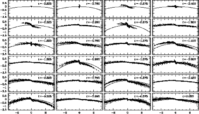
Fig. 6.—: Morphology of the simulated tidal tail in the simulation with parameters $R_{\mathrm{t}}=10\,$kpc, $W_{0}=2.75$, and $M_{0}=20000\,M_{\odot}$ (also called ‘model A’) at various times, given in Gyr in each panel. For every tenth body, we plot the position (in kpc) projected onto the instantaneous orbital plane of the cluster, whose motion is towards the right in each panel. The thin line indicates the cluster orbit.

The linear mass loss is accompanied by an average decrease in velocity dispersion. In the right panels of Fig. 4, we plot the virial radius

$$r_{\mathrm{vir}}\equiv GM/\sigma^{2}$$ (7)

of the stars within the initial limiting radius of the cluster. For most simulated clusters that survive until the present time, we find a modest decrease of the virial radius. In the top right panel of Figure 5, we plot the relative shrinking rate, $-\dot{r}_{\mathrm{vir}}/r_{\mathrm{vir}}(t=0)$, versus $W_{0}$ for various values of $R_{\mathrm{t}}$ but fixed $M_{0}$ (the dependence on $M_{0}$ is very weak at fixed $R_{\mathrm{t}}$ and $W_{0}$). Most model clusters shrink slightly in response to the disk shocks with a rate that is primarily a function of $W_{0}$, or, equivalently, of the initial cluster concentration. Only very low-concentration clusters do not shrink but may even expand, see also the lower two simulations in Fig. 4. The top left panel of Figure 5 plots the relative rates versus each other. While there is a clear tendency for mass loss to anti-correlate with shrinking, the spread in this diagram is considerable.

We like to point out that the shrinking rates are very small, of the order of a few percent per Gyr, too small to protect the cluster from continued tidal stripping, i.e. self-limitation of disk shocks does not apply here, as is also evident from the undamped mass-loss rates.

3.5 Tidal Tail Morphology

The stars lost from the cluster form two tidal tails, one leading the cluster and one trailing it. We will discuss the dynamics of the tidal tail in detail in the next section. Here, we want to give an impression of the morphology of these tails.

For the model whose remnant cluster best fits Pal 5 (see section 5.1), hereafter ‘model A’, Figure 6 shows snapshots of (one out of ten) stars in tail and cluster: the particle distribution projected onto the (instantaneous) orbital plane at time intervals of 125 Myr. At the first time shown, the cluster has not yet been tidally shocked and all the particles are still inside the cluster, after that, the two tails develop.

There are several notable observations possible from this Figure. First, near the cluster, the tail shows the typical S-shape, also visible in the observations of Pal 5, which originates from the trailing tail being at larger and the leading tail at smaller distance from the Galactic center.

Second, the tail morphology varies between thin and long near perigalacticon (e.g. $t=-0.45\,$Gyr), and short and thick near apogalacticon (e.g. $t=-2.075$, $-0.075\,$Gyr), which is due to variations of the orbital velocity and hence the separation between tail stars and cluster. This is analogous to cars on a motorway: slow driving with short separations as in a traffic jam and fast driving with large distances correspond to the situations near apogalacticon and perigalacticon, respectively.

Third, the tail neatly huddles against the cluster orbit at most of the times; only rarely near apogalacticon do some stars of the trailing (leading) tail appear closer (further). Fourth, occasionally near apogalacticon, the tidal tail shows a streaky structure. Each of these streaks corresponds to a swarm of stars that has been set loose by the same disk shock and fills apparently a streak-like phase-space volume, which occasionally projects also onto a streak in configuration space shown in the Figure.

4 The Dynamics of Tidal Tails

The gravitational influence of the cluster ceases not abruptly beyond its tidal radius, but it is completely negligible for stars that have drifted away from the cluster by more than a few tidal radii. Similarly, the self-gravity within the tidal tail is unimportant, simply because the tidal-tail stars move too fast w.r.t. each other. Thus, to very good approximation, the motion of a tidal tail star is governed by the gravitational potential $\Phi$ of the Milky Way only.

For a time-invariant and smooth Galactic gravitational field, such as adopted in the simulations (but see section 7.3 for a discussion of deviations from this ideal), a tidal-tail star moves on a Galactic orbit which is very similar to that of the cluster itself. The offset in orbital energy may be estimated to be (Johnston, 1998)

$$\delta E_{\mathrm{{orb}}}\simeq\pm\;r_{\mathrm{tid}}\;|\boldsymbol{\nabla}\Phi|.$$ (8)

This follows from the fact that when the star leaves the cluster its cluster-internal energy approximately vanishes and its velocity is very similar to that of the cluster, which leaves only the difference in potential energy as significant contribution to $\delta E_{\mathrm{{orb}}}$.

In reality, the star may leave the cluster with a higher than just escape energy, and $|\delta E_{\mathrm{{orb}}}|$ follows a distribution with a tail to larger values, but in any case $|\delta E_{\mathrm{{orb}}}|\ll|E_{\mathrm{orb}}|$. Thus, a star in the tidal tail moves on an orbit with slightly higher (lower) orbital energy than the cluster, and hence slightly longer (shorter) orbital period. Over time, the longer (shorter) orbital period results in a lag (lead) of the star w.r.t. the cluster, i.e. positive and negative $\delta E_{\mathrm{{orb}}}$ result in a trailing and leading tidal tail, respectively. Since the trailing tail moves on a higher orbital energy, it has a larger radius.

If we assume that a tail star leaves the cluster at a larger or smaller galactocentric radius, but the same Galactic azimuth and latitude, and the same velocity as the cluster, then we expect it to have the same orbital eccentricity as the cluster and to move in the same orbital plane (paper II). In reality, we expect deviations from this ideal, but, of course, the orbital eccentricity and inclination should only slightly differ from that of the cluster orbit.

4.1 Coordinates for Tidal-Tail Stars

Since the orbits of a tidal-tail star and of the cluster are so similar, the position of a tail star may be referred to the cluster’s trajectory. In paper II, we gave a simple model for the kinematics of stars in the tail, which was based on the assumption that its orbit has the same eccentricity as that of the cluster and differs only in energy. If we further assume that the Milky Way has a flat rotation curve, we have

$$\frac{|\delta\boldsymbol{x}|}{|\boldsymbol{x}_{\mathrm{orb}}|}\approx\frac{|\delta P|}{P}$$ (9)

where $\delta P$ is the difference between the orbital period of the tail star and the period $P$ of the cluster, while $\delta\boldsymbol{x}\equiv\boldsymbol{x}-\boldsymbol{x}_{\mathrm{orb}}$ is the positional offset of a tail star from the cluster trajectory at the same orbital phase, not the same time, see Fig. 7 for an illustration.

Fig. 7.—: Illustration for the definition of tail coordinates, see section 4.1 for details.

Since at the same phase $\delta\boldsymbol{x}\parallel\boldsymbol{x}_{\mathrm{orb}}$, equation (9) gives a simple relation between the perpendicular positional offset of the tail star from the cluster trajectory and the period difference, which is directly related to the positional offset along the trajectory. In paper II, we used this simple relation to estimate the mean drift rate, and consequently the mass-loss rate, from the mean radial orbital offset of the tidal tail of Pal 5 from its orbit. For a flat-rotation-curve Galaxy, we further have (for $\delta P\ll P$)

$$\frac{\delta P}{P}=\exp\left(\frac{\delta E_{\mathrm{{orb}}}}{v_{\mathrm{c}}^{2}}\right)-1\approx\frac{\delta E_{\mathrm{{orb}}}}{v_{\mathrm{c}}^{2}}.$$ (10)

Fig. 8.—: Distribution of tidal-tail stars over the dimensionless drift rate $\eta$, time $t_{\mathrm{l}}$ of loss from the cluster, and orbital energy offset $\delta E_{\mathrm{{orb}}}$ from the cluster. The values are obtained at $t=0$ from model A ($R_{\mathrm{t}}=10\,$kpc, $W_{0}=2.75$, and $M_{0}=20000\,M_{\odot}$). Tidal-tail stars with $t_{\mathrm{l}}>-0.2\,$Gyr have been omitted. The thin lower histogram in the bottom right panel is for stars with $t_{\mathrm{l}}\in[-2.5,-2.4]\,$Gyr. In the upper right panel only one out of four bodies is plotted.

Motivated by this model, we now introduce simple coordinates for stars in the tidal-tail. For a tail star at position $\boldsymbol{x}$, we first find the reference point $\boldsymbol{x}_{\mathrm{orb}}$ on the local cluster orbit by minimizing $|\boldsymbol{x}\times\boldsymbol{x}_{\mathrm{orb}}(\tau)|$ w.r.t. the time parameter $\tau$ along the cluster orbit, see Figure 7 for an illustration. With $\tau$ defined such that $\boldsymbol{x}_{\mathrm{orb}}(0)=\boldsymbol{x}_{0}$, we can use the time $\tau$ directly as the tail star’s (relative) coordinate along the tail. For the trailing (sketched in Fig. 7) and leading stars, $\tau<0$ and $\tau>0$, respectively. Note that, in contrast to the true positional offset between cluster and tail stars, $\tau$ is not subject to ‘seasonal’ variations between apogalacticon and perigalacticon seen in Fig. 6, since these are caused by variations in orbital velocity.

As further coordinates we use the components

$$\delta x_{\parallel} \equiv \delta\boldsymbol{x}\cdot\boldsymbol{x}_{\mathrm{orb}}/|\boldsymbol{x}_{\mathrm{orb}}|,$$ (11a)

$$\delta x_{\perp} \equiv \delta\boldsymbol{x}\cdot\boldsymbol{L}_{\mathrm{orb}}/|\boldsymbol{L}_{\mathrm{orb}}|,$$ (11b)

of $\delta\boldsymbol{x}$ parallel to $\boldsymbol{x}_{\mathrm{orb}}$ (in the orbital plane) and parallel to the angular momentum vector $\boldsymbol{L}_{\mathrm{orb}}\equiv\boldsymbol{x}_{\mathrm{orb}}\times\dot{\boldsymbol{x}}_{\mathrm{orb}}$ (perpendicular to the orbital plane and the paper in Figs. 6 and 7).

We may go a step further and define the dimensionless coordinates

$$\eta \equiv \tau/(t-t_{\mathrm{l}}),$$ (12a)

$$\zeta_{\parallel} \equiv \delta x_{\parallel}/|\boldsymbol{x}_{\mathrm{orb}}|,$$ (12b)

$$\zeta_{\perp} \equiv \delta x_{\perp}/|\boldsymbol{x}_{\mathrm{orb}}|,$$ (12c)

where $t_{\mathrm{l}}$ is the time when the star was lost from the cluster. $\eta$ essentially is a dimensionless drift rate, while $\zeta_{\parallel}$ and $\zeta_{\perp}$ are dimensionless offsets in and out of the orbital plane.

The time $\tau$ corresponds to a phase difference $\delta\theta=\tau\omega$, which originates from the frequency difference $\delta\omega$ acting over the time $t-t_{\mathrm{l}}$, i.e. $\delta\theta=(t-t_{\mathrm{l}})\delta\omega$. We thus have $\eta=\delta\omega/\omega=-\delta P/P$ and equations (9) and (10) yield

$$\zeta_{\parallel} \approx -\eta$$ (13a)

$$-\eta \approx \delta E_{\mathrm{{orb}}}/v_{\mathrm{c}}^{2}$$ (13b)

and $\zeta_{\perp}\approx 0$. That is, not only should these coordinates be conserved, i.e. all the kinematics is contained in their construction, but they are related in a very simple way. However, the model on which equation (9) is based ignores differences in orbital eccentricity and inclination between tail-star and cluster. Since the orbital period is mainly a function of orbital energy, whereas the orbital position at fixed phase also depends sensitively on the eccentricity and inclination, we expect deviations from our ideal to mainly affect (13a) and $\zeta_{\perp}\approx 0$, but not so much (13b).

4.2 Kinematics of the Tidal Tail

We are now going to investigate in some detail the distribution of tidal-tail stars over the relative coordinates $(\eta,\,\zeta_{\parallel},\,\zeta_{\perp})$, $\delta E_{\mathrm{{orb}}}$, and $t_{\mathrm{l}}$, thereby also testing the simple relations (13) above. For this purpose, we concentrate on the one simulation already used in Fig. 6 above, which is one that gives a good description of Pal 5 (see Section 5). In this model the cluster originally had $r_{\mathrm{lim}}=53\,$pc.

In the top left panel of Figure 8, we plot the dimensionless drift rate $\eta$, computed at the end of the simulation, vs. the time $t_{\mathrm{l}}$ of loss from the cluster (evaluated as the last instant when the star crossed $r_{\mathrm{lim}}$ outwards). Clearly, each disk shock triggers the loss of a swarm of stars with a spread in $\eta$ which is almost symmetric for trailing and leading tail. The morphology in ($\eta,t_{\mathrm{l}}$) of each of these shocks is the same. First the stars with largest $|\eta|$ escape, because they have highest velocity, and somewhat later those with smaller $|\eta|$. The smallest $|\eta|$ of any tail star decreases towards later times, because the cluster loses mass and escaping from it becomes easier.

The drift rates $\eta$ follow a broad distribution with a factor of four between minimum and maximum. Therefore, a swarm of tail stars set loose by one disk shock quickly disperses along the tail. In particular, the fastest drifting tail stars will soon run into the slowest drifting ones lost at the previous shock. This implies that at any distance from the cluster the tail is a superposition of stars lost at various epochs, illustrated also in Fig. 10 below. We may estimate the number of shocks contributing to the tidal tail at some ‘distance’ $\tau$ by dividing the difference between maximum and minimum $t-t_{\mathrm{l}}$ by the average time $t_{\mathrm{disk}}$ between shocks

$$n\approx(\eta_{\mathrm{min}}^{-1}-\eta_{\mathrm{max}}^{-1})\frac{\tau}{t_{\mathrm{disk}}}\sim\frac{3}{4\eta_{\mathrm{min}}}\frac{\tau}{t_{\mathrm{disk}}}.$$ (14)

With $\eta_{\mathrm{min}}\sim 0.005$ and $t_{\mathrm{disk}}\approx 300\,$Myr, this gives $n\sim 0.5(\tau/$Myr). For the current situation of Pal 5, this translates into $n\sim 2(l/$deg) with angular separation $l$ from the cluster (assuming $v_{\mathrm{orb}}\sim 100\,$km s^-1 for the cluster’s orbital velocity).

The maximum drift rate is still rather low: about 2 percent, i.e. it would take $\sim 50$ orbits $\sim 15\,$Gyr for the fastest first escapees to cover a full orbital period, i.e. to fill a great circle on the sky.

The top-right panel of Fig. 8 shows that there is indeed a tight relation between $\delta E_{\mathrm{{orb}}}$ and $\eta$, as expected from our equation (13b). However, there is a considerable spread, in particular at small $|\eta|$, which persists if we restrict the analysis to larger $|t_{\mathrm{l}}|$ (excluding stars still in the neighbourhood of the cluster). There is also a systematic deviation in the sense that the linear relations for the trailing and leading tail have non-vanishing zero points.

The bottom panels of Fig. 8 show histograms of $t_{\mathrm{l}}$, i.e. the mass-loss rate, and $\delta E_{\mathrm{{orb}}}$. A comparison with Fig. 3 shows that the amount of mass lost in a shock correlates with the strength of the tidal field, as expected. The distribution in $\delta E_{\mathrm{{orb}}}$ is, of course, a superposition of the distributions created by each of the disk shocks and the thin histogram shows the distribution from the single shock at $-2.45\,$Gyr. The fact that the inner edge of the distribution (towards small $|\delta E_{\mathrm{{orb}}}|$) is not abrupt is mainly due to the fact that the cluster weakened with time, allowing smaller $|\delta E_{\mathrm{{orb}}}|$ at later epochs. The typical scale for $\delta E_{\mathrm{{orb}}}$ is $\sim 300\,$(km s${-1}$)$2$. This value indeed follows from equation (8) for a cluster with $r_{\mathrm{tid}}\sim 60\,$pc at $R\sim 10\,$kpc in a logarithmic potential with $v_{\mathrm{c}}\sim 220\,$km s^-1. The distribution in $\delta E_{\mathrm{{orb}}}$ is not quite, but still remarkably symmetric.

Fig. 9.—: Plots of $\zeta_{\perp}$ (top) and $\zeta_{\parallel}$ (bottom) vs. $\eta$ for model A (the same as in Fig. 8) at $t=0$ (left, near apocenter) and $t=-0.45\,$Gyr (right, near apocenter). The thin lines indicate the relations (13a) and $\zeta_{\perp}=0$, which are expected from naive modeling. For clarity, only one out of four bodies is plotted.

In Figure 9, we plot the dimensionless orbital offsets $\zeta_{\parallel}$ and $\zeta_{\perp}$ vs. $\eta$ computed at two different epochs, once near apogalacticon and once near perigalacticon. Quite obviously, the relation $\eta\approx-\zeta_{\parallel}$ (13a) does not generally hold, only for the trailing tail at $t=0$ we find reasonable agreement. We also find that $\zeta_{\perp}$ deviates from zero substantially in the sense that typical values are significant compared to $\eta$. A comparison between the two epochs clearly shows that $\zeta_{\parallel}$ and $\zeta_{\perp}$ are in fact not conserved. This, together with the violation of $\zeta_{\parallel}\approx-\eta$ and $\zeta_{\perp}\approx 0$ implies, in accordance with the discussion following equations (13), that the orbital eccentricities and inclinations of tail stars differ significantly and systematically from that of the cluster. On the other hand, $\delta E_{\mathrm{{orb}}}$ shows only marginal changes with time (not shown in a Figure), while $\eta$ changes significantly with time, but still much less than 100%, in contrast to $\zeta_{\parallel}$ and $\zeta_{\perp}$.

We may thus conclude that in practice the dimensionless drift rate $\eta$ is reasonably well conserved and correlates well with $\delta E_{\mathrm{{orb}}}$, while $\zeta_{\parallel}$ and $\zeta_{\perp}$ are subject to substantial time evolution. These conclusions are supported by all simulations, not just the one presented in Figures 8 and 9.

Fig. 10.—: Distribution of tidal-tail stars in $\tau$ and time $t_{\mathrm{l}}$ of loss from the cluster for model A (the same as in Fig. 8). The two vertical lines bracket the range in $\tau$ inaccessible to stars with $t_{\mathrm{l}}<-2.95\,$Gyr. That is, stars lost prior to the start of the simulation, which are, of course, not contained in our model, contribute only to $|\tau|>19\,$Myr.

4.3 Stellar Density along the Tail

The linear stellar density $\varrho=\mathrm{d}M/\mathrm{d}s$ along the tail, or, similarly, the circularly averaged surface density $\Sigma(R)$ of stars (tail & cluster) are easily observable from Pal 5 (see Fig. 2, paper II). A study by Johnston, Sigurdsson & Hernquist (1999) of the formation of tidal tails due to Galactic tides acting on globular clusters or satellite galaxies suggest that $\Sigma\propto R^{-1}$, or equivalently $\varrho\approx\mathrm{const}$

We may identify three factors that determine $\varrho(s)$: the mass-loss rate $\dot{M}$; the distribution $f(\eta)$ of dimensionless drift rates, which may be a function of the time $t_{\mathrm{l}}$ of loss from the cluster; and the orbital kinematics that map the phase-distance $\tau$ into physical distance $s$ along the orbit. The first two factors, which depend mainly on the general properties of the orbit (period and perigalactic radius) and the cluster, determine the distribution of tail stars over $\tau$

$$\frac{\mathrm{d}M{}}{\mathrm{d}\tau}=\int_{-\infty}^{t}\!\mathrm{d}t_{\mathrm{l}}\;\dot{M}(t_{\mathrm{l}})\int_{-\infty}^{\infty}\!\mathrm{d}\eta\;f(\eta;t_{\mathrm{l}})\;\delta\big{(}\tau-\eta(t-t_{\mathrm{l}})\big{)}.$$ (15)

The last factor depends on the current position on the orbit and yields

$$\varrho(s;t)=\frac{1}{|\boldsymbol{v}_{\mathrm{orb}}(\tau)|}\frac{\mathrm{d}M{}}{\mathrm{d}\tau}$$ (16)

where $s=\int_{0}^{\tau}|\boldsymbol{v}_{\mathrm{orb}}(\tau^{\prime})|\,\mathrm{d}\tau^{\prime}$ calculated at the current time $t$.

A constant $\varrho(s)$, such as found in the simulations by Johnston et al., emerges from a constant (orbit-averaged) $\dot{M}$ in conjunction with a time-invariant distribution $f(\eta)$ of drift rates and $|\boldsymbol{v}_{\mathrm{orb}}|\approx\mathrm{const}$ over the extent of the tail. This latter condition is not satisfied whenever the tidal tail spans a significant range in phases on an eccentric orbit.

As we saw in Fig. 8, the distribution over drift rates $\eta$ is actually not time invariant for our models: the drift rates decrease, because the cluster is significantly weakened by the continued loss of stars. With a constant (orbit averaged) mass-loss rate, this results in $\mathrm{d}M/\mathrm{d}\tau$ slightly decreasing with $|\tau|$. This is illustrated in Figure 10, which plots the distribution of tail stars over $\tau$ and $t_{\mathrm{l}}$. In the top panel, it is evident that the typical $|\tau|$ increases slightly faster than linear with $t-t_{\mathrm{l}}$ (the inner envelopes are not straight lines). The plot of $\mathrm{d}M/\mathrm{d}\tau$ in the bottom panel shows (i) some ‘bumpiness’ at the $\lesssim 20\%$ level and (ii) a slight decrease with $|\tau|$ (data for $|\tau|>19\,$Myr are incomplete since tail stars with $t_{\mathrm{l}}<-2.95\,$Gyr are lacking from our models, see also the discussion at the end of section 3.2). For the linear density $\varrho$, the latter implies a slight decrease with $s$ and a steeper than $R^{-1}$ decrease for $\Sigma$. Thus, we expect non-constant $\varrho(s)$ even for a (orbit-averaged) constant mass-loss rate and a tail spanning a small range of $|\boldsymbol{v}_{\mathrm{orb}}|$, if the mass loss was substantial.

For clusters or satellites which undergo only non-substantial mass loss, the distribution over $\eta$ should indeed be independent of time and consequently $\mathrm{d}M/\mathrm{d}\tau\approx\mathrm{const}$, consistent with the results of the aforementioned study by Johnston et al..

The bumpiness of $\mathrm{d}M/\mathrm{d}\tau$, which of course translates in a bumpiness of $\varrho(s)$, is caused by individual shocks and the fact that for small $\tau$ only few of them contribute. These bumps are expected to be symmetric, i.e. occur in trailing and leading tail at about the same distance from the cluster. For larger $\tau$ or distances $s$ from the cluster these inhomogeneities are averaged out by the superposition of many swarms of stars lost from the cluster at different shock events.

4.4 Drift Rates and Tail Kinematics of the Models

In order to investigate the dependence of the tail properties on the model parameters, we computed for each model of a cluster that survived until today the mean and dispersion of $\eta$, $\zeta_{\parallel}$, $\zeta_{\perp}$, and $\delta E_{\mathrm{{orb}}}$ evaluated at $t=0$ for both the leading and trailing tail.

Fig. 11.—: For all 695 simulations with a cluster surviving until $t=0$, we plot against each other: the average offset in orbital energy $\delta E_{\mathrm{{orb}}}$ between tail stars and cluster; the average absolute dimensionless drift rate $\eta$; and the weighted mean of the initial and final mass of the cluster. $\delta E_{\mathrm{{orb}}}$ and $\eta$ have been calculated at $t=0$. The thin curves in the two left panels follow a power-law with exponent $1/3$.

The estimate (8) for $\delta E_{\mathrm{{orb}}}$ suggests that $\langle|\delta E_{\mathrm{{orb}}}|\rangle$ depends only on the mass $M$ of the cluster at the instant of the star leaving it. Because our models are subject to substantial mass loss, their mass is not conserved. However, as the bottom-left panel of Figure 11 demonstrates, the average $\langle|\delta E_{\mathrm{{orb}}}|\rangle$ over all tail stars (lost over the whole integration interval) is strongly correlated with some time-averaged cluster mass. In fact $\langle|\delta E_{\mathrm{{orb}}}|\rangle\propto M^{1/3}$, exactly as equations (8) and (1) predict. The constant of proportionality in this relation depends on the cluster orbit and the Galactic potential only, but not on the cluster’s intrinsic properties. The remaining two panels of Fig. 11 show that the mean dimensional drift rate $\langle|\eta|\rangle$ is proportional to $M^{1/3}$, too, and to $\langle|\delta E_{\mathrm{{orb}}}|\rangle$. The constant of proportionality in this latter relation is $(196\,$km/s)^-2, corresponding approximately to $v_{\mathrm{c}}^{-2}$, in accordance with equation (13b).

With this mass dependence, we obtain for the average density of tail stars over $\tau$ from equation (15)

$$\left\langle\frac{\mathrm{d}M}{\mathrm{d}\tau}\right\rangle\propto\frac{M}{\langle\eta\rangle}\propto M^{2/3}$$ (17)

with $M$ denoting some measure of the cluster mass (final or time averaged). The constant of proportionality depends on the relative mass-loss rate $\dot{M}/M_{0}$ and hence is a function of $R_{\mathrm{t}}$ and $W_{0}$, but hardly of $M_{0}$. Thus, at fixed $(R_{\mathrm{t}},W_{0})$, a smaller cluster mass results in a larger fraction of tail stars at fixed $\tau$, i.e. phase offset from the cluster.

5 Comparison with Pal 5

In this section we compare the 695 models with a surviving cluster to the observed properties of Pal 5 and its tail. The objective is to investigate whether these data are at all consistent with our models and if so, with which type of models.

Fig. 12.—: Distribution of the 695 simulated clusters over the fractions of stars within projected $16\arcmin$ that are also within projected $4\arcmin$ (x-axis) and $12\arcmin$ (y-axis). Note that $16\arcmin$ is the limiting radius of Pal 5 itself, whose data are shown as solid square. The open square marks the model which best fits the data for Pal 5 and is denoted ‘model A’ in the text.

5.1 The Cluster

The most astonishing property of Pal 5, apart from the tails, is its size, which is about four times larger than expected for a cluster of its mass and on its orbit (section 2.3). Instead of comparing 695 different projected surface density profiles, we plot in Figure 12 the fractions of the projected cluster mass within $16\arcmin$ (the limiting radius of Pal 5), that are also within the projected radii of $4\arcmin$ and $12\arcmin$. Most of our models are in the upper-right corner of the figure: they have nearly $100\%$ for both these fractions, meaning that most of their mass is contained within $4\arcmin$, the tidal radius of Pal 5 at perigalacticon. Thus, these simulated clusters have survived until today, because they are, in contrast to Pal 5, smaller than their tidal radii.

There is, however, also a long tail of models with lower mass fractions within $4\arcmin$ and $12\arcmin$, corresponding to larger extents. Some of these actually come close to Pal 5 in the sense that they have $\sim 95\%$ of their mass within $12\arcmin$ and $\sim 60\%$ within $4\arcmin$. These models have initial parameters $W_{0}\simeq 2-3$, $R_{\mathrm{t}}\simeq(4.5+2W_{0})\,$kpc, and $M_{0}\simeq 20000\,M_{\odot}$, while model clusters with $R_{\mathrm{t}}$ larger than that (at fixed $W_{0}$) get destroyed and those with lower mass are even more diffuse or have been disrupted as well. Initially more concentrated models with $W_{0}\gtrsim 3$ and also $R_{\mathrm{t}}\simeq(4.5+2W_{0})\,$kpc form the tail in Fig. 12 towards smaller mass fractions; they have massive tidal tails but their clusters are not as extended as Pal 5.

The model that best matches Pal 5 in Fig. 12 is that with initial parameters $R_{\mathrm{t}}=10\,$kpc, $W_{0}=2.75$, and $M_{0}=20000\,M_{\odot}$; it is marked with an open square and will be denoted ‘model A’. This model already featured in Figures 6, 8, 9, and 10 and will be used in the remainder of the paper for illustrative purposes.

Fig. 13.—: Time evolution of mass (top) and velocity dispersion (bottom) of model A (with $R_{\mathrm{t}}=10\,$kpc, $W_{0}=2.75$, and $M_{0}=20000\,M_{\odot}$). The dotted vertical lines are equivalent to those in Fig. 4. The cluster is destroyed by the first future disk crossing at $t=110\,$Myr.

Fig. 14.—: Distribution of the 695 simulated clusters over the final projected mass within 16′and the line-of-sight velocity dispersion within 6′. Larger symbol sizes correspond to models that are closer to Pal 5 in their enclosed projected mass fractions (Fig. 12); the largest symbol refers to model A. Note that for Pal 5, $M_{r<16\arcmin}=5200\pm 700M_{\odot}$ and $\sigma_{\mathrm{los},r<6\arcmin}=0.22^{+0.19}_{-0.10}\,$km s^-1 (assuming a Gaussian distribution, see also Fig. 15 and the text for a discussion).

Figure 13 shows the time evolution of the cluster mass and velocity dispersion $\sigma$ of model A. All models which come close to Pal 5 in their projected mass fractions in Fig. 12 show substantial mass loss, which results in a drastic increase in the cluster’s dynamical time $t_{\mathrm{dyn}}$, reflected by the steady decline of $\sigma$. The increase of $t_{\mathrm{dyn}}$ slows down the cluster’s response to disk shocks: the period of the (damped) oscillations that follow each shock (in Fig. 13 visible as oscillations of $\sigma$ subsequent to each dotted vertical line, see also the discussion in section 3.4.1) increases. Eventually, this period approximately equals twice the time between two shocks, namely those at $t=-146$ and 110 Myr, such that just in the middle between these two shocks, i.e. today, the cluster is in state of maximal expansion and minimal velocity dispersion. This property is common to all models with projected density profile similar to that of Pal 5.

Thus, all those models that reproduce the overly large extent of Pal 5 also naturally, and causally connected, predict a very small velocity dispersion consistent with that actually observed for Pal 5.

Fig. 15.—: Top: distribution over distance $r$ from the Sun and line-of-sight velocity for stars within projected 6′ of the cluster center for the final state of model A (initial parameters: $W_{0}=2.75$, $R_{\mathrm{t}}=10$, and $M_{0}=20000M_{\odot}$). Bottom: distribution of the same stars over $v_{\mathrm{los}}$ and a Gaussian with $\sigma_{\mathrm{los}}=0.38\,$km s^-1 (dotted).

Fig. 16.—: Distribution of the 695 simulated tails with surviving clusters over ($x$-axis) the ratio between mass in the tail out to projected $200\arcmin$ and the mass in the cluster (within $16\arcmin$) and ($y$-axis) the fraction of tail stars within $100\arcmin$ for the trailing (top) and leading (bottom) tail, respectively. The symbol sizes indicate how well the model matches the cumulative projected masses of the cluster (Fig. 12). The solid square represents the star-count data for Pal 5, which have a statistical uncertainty of about 0.05 in the $y$ direction. The trailing tail of Pal 5 has a substantial clump at 3 deg from the cluster, compromising the measures plotted, in particular that on the $y$ axis.

In Figure 14, we plot for all 695 surviving cluster models the final mass within projected 16′ (the limiting radius of Pal 5) and velocity dispersion of stars within projected 6′. The models with projected mass profiles most similar to Pal 5 (shown as larger symbols) form the lower envelope, i.e. have lowest line-of-sight velocity dispersion $\sigma_{\mathrm{los}}$ at given projected mass. A direct comparison of these values for $\sigma_{\mathrm{los}}$ with that determined for Pal 5 in paper I (see section 2.2) is problematic, as the latter has been obtained under the assumption that the line-of-sight velocity distribution was Gaussian (high-velocity tails have been modeled as binary contamination).

In Figure 15, we show for the model that best fits the projected mass profile (the biggest symbol in Fig. 14) the distribution of stars within projected 6′ of the cluster center over distance $r$ and line-of-sight velocity $v_{\mathrm{los}}$. The dotted line in the lower panel represents a Gaussian with $\sigma_{\mathrm{los}}=0.38\,$km s^-1. Clearly, the distribution has non-Gaussian wings, which originate from stars that are just being lost from the cluster. Thus, the extra-Gaussian tails of the observed line-of-sight velocity distribution can at least partly be explained by cluster dynamics and not entirely by binaries, as we assumed in paper I.

The very model shown in Fig. 15 not only gives the best fit to the shape of the Pal 5’s mass-profile, but also its total mass within 16′ of 5177 $M_{\odot}$ agrees nicely with the best estimate for Pal 5 of $5200\pm 700\,M_{\odot}$ (section 2.2).

5.2 The Tidal Tail

5.2.1 The Radial Profile

Fig. 17.—: Distribution of the 695 simulated tails with surviving clusters over ($x$-axis) the mean projected drift rate along the orbits and ($y$-axes) the mean (bottom) and dispersion (top) of the rectangular displacement $p$ of the tail stars from the orbit. Only tail stars with distance (projected arc-length $s$ along the tail) from the cluster within $[24\arcmin,\,200\arcmin]$ have been used. The symbol sizes indicate how well the model matches the cumulative projected masses of the cluster (Fig. 12). See text for a comparison with Pal 5

In Figure 16, we compare the gross radial distribution of stars in the tail of Pal 5 with those of the 695 models with surviving clusters. On the $x$-axis, we plot, for the trailing (top) and leading (bottom) tidal tail, the ratio of tail to cluster mass. Here, we rather arbitrarily truncated the tail at $200\arcmin$ to ensure that no stars are missing from the simulations due to our limited integration time (cf. the discussion following Fig. 10). On the $y$-axis of Fig. 16, we plot the fraction of the tail mass within $100\arcmin$. This fraction is related to the density run along the tail: for a constant linear density, equivalent to $\Sigma\propto r^{-\gamma}$ with $\gamma=1$, we expect $\sim 0.46$, while steeper density profiles with $\gamma>1$ yield larger values.

We first notice a weak correlation between this ratio and the relative mass in the tail in the sense that (relatively) more massive tails have higher fractions of stars inside $100\arcmin$, corresponding to larger $\gamma$. This is, of course, exactly what we expect from our discussion in §4.3.

Regarding Pal 5, we see that while its leading tail falls into the locus of models, the trailing tail does not. This can be entirely attributed to the clump at $\sim 3^{\circ}$ from the cluster (paper II, see also Fig. 2). We also notice that those models which best fit the properties of the cluster itself (indicated by larger symbol sizes in Fig. 16), have tails that are more massive by a factor 1.5 – 2 and have a steeper radial density profile (but note that the statistical uncertainty on this latter property of Pal 5 is considerable).

We should note here that for Pal 5, we actually cannot measure mass ratios, but merely number count ratios, which are identical to the former only, if the stellar luminosity functions (LFs) in the cluster and the various parts of the tail are the same. Actually, Koch et al. (2004) reported a significant lack of low-mass stars in the cluster as compared to its tails, which may explain (at least partly) the apparent discrepancy in the tail-to-cluster mass ratio.

Thus, we conclude that simultaneous fitting of the projected radial profile of Pal 5 and its tails appears to be difficult, while each property on its own is inside the locus of the models. However, statistical uncertainties and our lack of knowledge of mass (rather than number-count) ratios, i.e. of the LF, hampers more quantitative statements to be made.

Another important point is that the clumpiness of the tidal tail of Pal 5, in particular the over-density at $3^{\circ}$ in the trailing tail, is not reproduced in any of our models. We will discuss in section 7.3 the possible implication of this mismatch.

Fig. 18.—: Projection of model A at $t=0$ (today) onto the sky in standard Galactic coordinates (bottom) and plots of the offset in distance modulus (middle) and radial velocity (top) of the stars from the cluster versus Galactic longitude. The thin line represents the orbit. Only every second body is plotted.

5.2.2 The Offset from the Orbit

In paper II, we measured the projected rectangular offset of tail stars from the projected (assumed) orbit. In order to compare our simulations to these measurements, we computed the same quantities for our models (after projection onto the sky as seen from the Sun) as follows. First, we determined the point on the projected orbit that minimizes the projected distance to the tail star. We then define $p$ to be the projected distance with $p>0$ ($p<0$) for tail stars at larger (smaller) Galactic latitude than the nearest point on the orbit. We define $s$ to be the arc-length along the projected orbit with $s>0$ and $s<0$ for the leading and trailing tail, respectively.

In Figure 17, we plot, separately for the trailing (left) and leading (right) tails of the all the models with surviving cluster, the mean (bottom) and dispersion (top) of $p$ versus the mean projected drift rate $s/(t-t_{\mathrm{l}})$.

From this Figure, we see that, while the drift rates for the leading and trailing tail are of comparable size, the mean rectangular distance $|p|$ is larger by almost a factor of two for the former. This is also evident from the projection of model A in the bottom panel of Figure 18. The reason is partial intrinsic, i.e. due to the offsets $\zeta_{\parallel}$ of the tail stars from the cluster orbit within the orbital plane (Fig. 9, left bottom panel), and partly due to projection effects (because the leading tail is closer to us and seen under a slightly smaller inclination angle).

In contrast to the modeled tails, the values inferred in paper II for the mean rectangular offset of Pal 5’s tail stars are rather similar for the trailing and leading tail ($11{}^{\prime}\!.8\pm 0{}^{\prime}\!.5$ and $-10{}^{\prime}\!.1\pm 0{}^{\prime}\!.8$, respectively). However, this is essentially a consequence of the implicit assumption, made when adopting the orbit in paper II, that the rectangular offsets are similar in size between the two tails. The fact that the simulations consistently predict larger $\langle|p|\rangle$ for the leading than the trailing tail implies that the orbit of Pal 5 should actually be slightly different from the one used in paper II and here; compare, for instance, the bottom panel of Fig. 18 with Fig. 9 of paper II. (Note, however, that the uncertainty in the distance to Pal 5 still dominates the uncertainty in the orbit).

However, we may still compare the tails’ perpendicular structure to the models by means of the dispersion in $p$. In paper II, we fitted a Gaussian to the distributions in $p$ for the trailing and leading tails of Pal 5. When assuming that the distribution is actually Gaussian, we obtain for the dispersions $7{}^{\prime}\!.8\pm 0{}^{\prime}\!.5$ and $7{}^{\prime}\!.3\pm 0{}^{\prime}\!.8$ for the trailing and leading tail, respectively. Comparing these values with those in Fig. 17, it appears that the tail of Pal 5 is at the upper end of the distribution. In particular, these values are somewhat larger than those for the models that best fit the cluster’s cumulative mass distribution (big symbols in Fig. 17).

The mean drift rate estimated for the trailing and leading tail in paper II was $\sim 180\,$arcmin/Gyr, which is substantially more than predicted by the models, even by those with as high a dispersion in $p$ as observed for the tails of Pal 5. That estimate, however, was based on rather simplifying assumptions on the relation with $p$ and, given the model results in Fig. 17, a lower value for the mean drift rate seems more appropriate. In face of the uncertainties, we cannot make precise statements, except for saying that most likely the mean drift rate is in the range $100-140\,$arcmin/Gyr, implying that the average tail star at the end of the observed trailing and leading tail was lost from the cluster about $3\pm 0.5$ and $2.4\pm 0.4$ Gyr ago, respectively.

5.2.3 Clues for Further Observations of Pal 5

In Figure 18, we plot the projection of model A onto the sky as well as the distribution of stars in their radial-velocity and distance-modulus offset from the cluster as function of offset in Galactic longitude. A comparison of the projection of model A with Fig. 9 of paper II shows, as already discussed above, that the orbit chosen in paper II is presumably not quite correct. This is important for any application where the orbit geometry is derived from the tidal tail.

The other two panels of Figure 18 plot the observable radial velocity and the distance modulus for the tail stars versus their galactic longitude. A measurement of either of these quantities for a sufficient number of tidal tail stars would constrain the acceleration in the Galactic halo at Pal 5’s present position and hence directly give the mass of the Milky Way within $\approx 18\,$kpc, a quantity not very well known.

From this Figure, we see that the distance-modulus offset of the tails is larger than that of the orbit, simply because of the generic shape of the tidal tails (see Fig. 6). This enhances the signal when trying to measure this effect: over the currently observed arc-length of the tail (from about $-6$ to $4$ in $\Delta(\ell\cos b)$, see Fig. 9 of paper II) the distance modulus changes by about 0.25 mag. The levelling off of the $\Delta m$ at $\ell\sim 8^{\circ}$ is because this is close to the apogalacticon of the orbit. This implies that in order to constrain the orbit of Pal 5, and hence the directly mass of the Milky Way, distance-modulus determinations should focus on $\ell\lesssim 8^{\circ}$.

A similar effect is seen for the radial-velocity offset, which also shows a larger gradient than the orbit itself. The difference here is that the spread in $\Delta v_{r}$ at any fixed position is larger, but also that gradient is maximal at apogalacticon, in contrast to $\Delta m$ whose gradient vanishes there.

Both the gradient in $\Delta m$ and that in $\Delta v_{r}$ are roughly proportional to the circular speed $v_{c}$ of the Galactic halo at the position of Pal 5. Thus, in order to determine $v_{c}$ to 10% accuracy, one would need to determine the $\langle v_{r}\rangle$ at $\sim 5^{\circ}$ on either side of the cluster to about 4 km s^-1 accuracy. Note that more accurate individual measurements are not sensible, because of (1) the intrinsic width of the tail and (2) possible binarity of the tail stars. For a determination of $v_{c}$ to 10% accuracy from the distance moduli at, say $\sim 5^{\circ}$ on either side of the cluster, an accuracy of 0.02 mag is sufficient. Both these accuracy requirements are not beyond current capabilities and a determination of the mass of our host galaxy within 18.5 kpc to $10-20\%$ accuracy seems possible.

6 Discussion I:
Cluster Evolution Driven by Disk Shocks

Our simulations were originally intended to understand the evolution and dynamical status of the globular cluster Palomar 5, but are also important for understanding disk-shocking driven globular-cluster evolution in general.

The orbit of Pal 5 is rather eccentric with an apogalactic radius of about 19 kpc, near the cluster’s present location. It carries the cluster to a perigalactic radius as low as 5.5 kpc, which implies strong tidal shocks at disk-crossings near perigalacticon. For a low-concentration low-mass cluster like Pal 5, these shocks rather than internal processes (driven by two-body relaxation) dominate the dynamical evolution (Gnedin, Lee & Ostriker, 1999).

A strong disk shock puts the cluster out of dynamical equilibrium by unbinding some stars and changing the (cluster-internal) energies of all the others. In addition to this energy mixing, there is also a general heating of the cluster. In low-concentration low-mass clusters, like Pal 5, this all happens much faster than their dynamical time, i.e. the shocks are impulsive. In response to this instantaneous heating, the cluster expands on its dynamical time scale, then contracts again, expands and so on. These oscillations are damped, since the internal dynamical times of the stars differ so that they get out of phase, and after a few dynamical times the cluster is in a new dynamical equilibrium.

For very low-concentration clusters the internal dynamical times (1) are long and (2) do not differ much, so that the damping is less efficient. This implies that for these systems the settling into a new equilibrium may be forestalled by the next strong disk shock. Hence, these clusters will never be in an equilibrium state, but are continuously rattled by the repeated tidal punches.

6.1 Evolution of Extended Clusters

We find that these shocks can be very efficient in driving the cluster evolution and may destroy the cluster within a few orbital periods. The disruption is faster the lower the cluster’s concentration and the larger its size compared to its perigalactic tidal radius. Thus, at smaller Galactic radii, the lifetime of low-concentration clusters is lower because of both stronger shocks and shorter orbital periods.

We should emphasize here, that our models were not initially, and never became, limited by their tidal radii. This implies that globular clusters extending beyond their theoretical (perigalactic) tidal radius and orbiting on eccentric orbits on which they experience strong disk shocks, will not quickly be ‘tidally stripped’ down to their tidal limit. This result seems to be at odds with the general wisdom of globular cluster dynamics in general and with the results of Gnedin et al. in particular. These authors found, using Fokker-Planck simulations, that in response to disk shocking the clusters become more compact, which renders the shock-induced evolution self-limiting.

However, we nonetheless think that our results are correct and not contradicting previous knowledge. Our simulations differ in various ways from those of Gnedin et al., who consider disk shocks which are non-impulsive and rare (internal dynamical time much shorter than time between shocks). We attribute the difference in our findings mainly to the eccentricity of the orbit of Pal 5 as compared to that of NGC 6254 (the cluster studied by Gnedin et al.). After being shock-heated near perigalacticon, clusters on eccentric orbits approach their new equilibrium whilst being in the remote parts of their orbit, where the Galactic tidal field is much smaller (about ten times, see Fig. 3) than near perigalacticon, even away from the disk. As a consequence, the new equilibrium, which does not know anything about the conditions near perigalacticon, is not limited by the perigalactic tidal radius.

This mechanism should not be very sensitive to the typical dynamical time of the cluster, since almost by definition of the tidal radius, the dynamical time of the outer parts of the cluster never is much smaller than the orbital time.

We find that in response to the disk shocks the clusters shrink somewhat, except for very low-concentration clusters, which even expand, making them yet more vulnerable and accelerating their destruction. However, this shrinking is very modest, of the order of at most a few percent per orbit even for medium-concentration clusters, much too small to protect them from continued disk shocking. For clusters of higher concentration and/or on less (or more) eccentric orbits, further studies are needed to investigate under which conditions tidal-force driven cluster evolution is self-limiting.

One implication of this possibility of super-tidally limited globular clusters is that inferring the mass of the Milky Way from the limiting radii of globular cluster assuming they are tidally limited (King, 1962; Bellazzini, 2004) is at best dangerous and may under-estimate the mass of the Milky Way.

6.2 Implications for the Globular-Cluster System

Many studies of the evolution of globular clusters and globular-cluster systems (e.g., Vesperini & Heggie, 1997; Baumgardt & Makino, 2003; Fall & Zhang, 2001) assumed that the sizes of globular clusters are initially upwardly limited by their (perigalactic) tidal radius. This assumption is based on the idea that the galactic tidal force field quickly results in such a tidal limitation, even if the clusters were originally larger. In view of our results, this assumption appears not generally justified, at least not for clusters on eccentric orbits. This implies that the above studies have probably underestimated the importance of disk shocks for the evolution of globular-cluster systems.

Our simulations predict unambiguously that Pal 5 will not survive its next disk crossing in $\sim$ 110 Myr. If me make the assumption that there is a plausible initial condition that could have formed 10 Gyrs ago and is being disrupted on this orbit now, then the fact that we observe Pal 5 within the last per cent of its lifetime, suggests that we see only the last tip of a melting iceberg. The inner Milky Way may well have been populated with numerous low-concentration globular clusters, which by now have all been destroyed, except for those, like Pal 5, whose orbits have longer periods and carry them into the more remote parts of the Galaxy. Currently, we have little possibility of quantitatively assessing the initial amount of low-concentration and low-mass globular clusters of the Milky Way galaxy. If tidal tails can survive for a Hubble time (but see section 7.3), we may be able to identify the debris of destroyed clusters as narrow streams of stars, which in turn may be identifiable in deep photometric, astrometric and/or spectroscopic surveys such as SDSS, RAVE and GAIA.

6.3 Tidal Tails

Each disk shock triggers the loss of a number of stars: those which have been accelerated beyond their escape velocity. These stars emerge with orbits whose energy is either slightly above or below that of the cluster. This offset in orbital energy is small compared to the orbital energy of the cluster itself (of the order of one per cent), so that the stars are not dispersed all over the Galaxy, but stay in a trailing and leading tidal tail, depending on the sign of the energy offset. This offset in orbital energy translates into an offset in orbital period and hence in a drift away from the cluster with a rate of the order of one per cent, i.e. a full wrap-around requires $\mathcal{O}(100)$ periods.

The orbital-energy offsets follow a broad distribution resulting in a distribution of drift rates. This implies that stars which have been lost from the cluster at the same time will not stay together but disperse along the tail. At any distance from the cluster, the tail contains stars lost at various shock events.

A constant drift rate in conjunction with a constant mass-loss rate results in a constant linear density of stars in the tidal tail or, equivalently, to a surface density $\Sigma\propto r^{-\gamma}$ with $\gamma=1$. This seems to be the generic property of tidal arms that results from continued tidal shocking (Johnston, Sigurdsson & Hernquist, 1999). However, when, as a result of continued mass loss, the cluster mass and hence the escape velocity drops considerably, stars with ever lower orbital energy offsets and hence lower drift rate can escape. In this case, the surface density exponent may be $\gamma>1$, in agreement with our empirical findings.

7 Discussion II:
The State and Fate of Pal 5

7.1 Is Pal 5 in Equilibrium?

Our simulations were primarily aimed at understanding Pal 5, predominantly because it is observed to possess a massive tidal tail. Apart from these tails, the most unusual property of Pal 5, which however has not been hitherto noticed, is its enormous size. The cluster is two times larger than its present theoretical tidal radius and even four times larger than its perigalactic tidal radius. This property can in fact be reproduced by (some of) our simulations, and can be understood in terms of the expansion that immediately follows each strong disk shock. All our model clusters that can reproduce the present size (and mass) of Pal 5 are in a state of near-maximal expansion after the last disk shock which occurred $\sim$ 146 Myr ago.

Maximal expansion implies minimal kinetic energy, corresponding to a small velocity dispersion. Indeed, models that can reproduce cluster size and mass comparable to Pal 5 also have the smallest (line-of-sight) velocity dispersions of all models, namely $\sigma_{\mathrm{los}}\sim 0.45$ km s^-1. We cannot produce models with $\sigma_{\mathrm{los}}$ much smaller than that, apparently because the tidal field limits the lowest velocity dispersions possible for a surviving cluster on any given orbit.

The line-of-sight velocity distribution of the models is actually not Gaussian, but contains some high-velocity tails resulting from stars just leaving the cluster. Correcting for these, we find a Gaussian $\sigma_{\mathrm{los}}\approx 0.38$ km s^-1 for model A that best fits size and mass. This value is consistent with our observation for Pal 5 of $\sigma_{\mathrm{los}}=0.22^{+0.19}_{-0.10}\,$km s^-1 (paper I).

All models that are comparable to Pal 5 in their cumulative mass distribution also predict that the cluster will not survive the next disk crossing in $\sim$ 110 Myr. The models that best fit the cluster radial profile have a constant orbit-averaged mass-loss rate of $\sim 5000\,M_{\odot}$Gyr^-1. Extrapolating this back in time implies an original mass of $\sim 70000\,M_{\odot}$, though this may be an over-estimate, since the strength of the Galactic tidal field was probably weaker in the past.

7.2 The Tidal Tail

Our models also have massive tidal tails. However, models that best fit the properties of the cluster tend to have a fraction of stars in the tail within 200′ that is about $50-100$% higher than observed for Pal 5. Note however that in this comparison we essentially assumed implicitly that the cluster’s luminosity function equals that of the tail, which actually appears to be not quite correct (Koch et al., 2004).

In our best fitting cluster models, $\sim$ 55% of the tail stars within 200′ are also within 100′. This corresponds to a surface density exponent of $\sim$ 1.35 and is consistent with our observations of Pal 5 (paper II).

All our models have a rather smooth density distribution along the tail with structure of less than $\sim 20\%$ in amplitude. This is because, as mentioned in section 6.3 above, even though the stars are lost at discrete events, they quickly disperse along the tail, washing out the discreteness of their liberation from the cluster.

This property of the model tails is in clear contrast to the observations of Pal 5, in particular its northern tail, which possesses a substantial clump at about 3 deg and seems to fade away at $\sim$ 6 deg, corresponding to a drift time of only $\sim$ 3 Gyr (section 5.2.2).

7.3 What Causes Structure of the Tidal Tail?

Why does the tidal tail of Pal 5 show this significant structure? Obviously, it must be caused by something not accounted for in our models. Evidently our models lack any Galactic substructure, such as giant molecular clouds and spiral arms. Clearly, since the Galactic disk itself is rotating, different parts of the tidal tail encounter different substructure when crossing the disk. If the tail passes, say, a giant molecular cloud at a distance smaller than its length, different parts feel substantially different perturbations and the tail will develop some substructure.

Another potential source of Galactic substructure that may affect the tidal tail are clumps in the dark-matter halo, which are actually predicted by standard $\Lambda$CDM cosmology (e.g. Moore et al., 1999; Klypin et al., 1999), or any super massive compact halo objects, such as proposed by Lacey & Ostriker (1985). In fact, the very integrity of the tail of Pal 5 may impose useful upper limits on the amount, sizes, and masses of such possible dark substructure in the Milky Way halo.

8 Summary and Conclusions

In order to study the disk-shock driven evolution of low-concentration globular clusters in general and of Pal 5 in particular, we performed 1056 $N$-body simulations. All these have the same Galactic potential and orbit (that derived for Pal 5), but differ in the internal properties of the cluster: its initial concentration (measured by $W_{0}$ for our King models), mass, and size (corresponding to our $R_{\mathrm{t}}$ parameter).

Our simulations demonstrate that disk-shocks near perigalacticon are very efficient at driving the evolution of low-concentration globular clusters. In particular, the disk-shocking induced mass loss is not self-limiting, but continues at a constant (orbit-averaged) mass-loss rate without limiting the cluster

to its (perigalactic) tidal radius. This behaviour, which is at odds with previous results by Gnedin et al. (1999), is probably a consequence of the eccentric orbit, which enables the cluster to settle into a new equilibrium near apogalacticon, i.e. unaffected by the perigalactic tidal field.

Our findings imply that initially not tidally limited clusters of low to medium concentration and moving on eccentric orbits may never become tidally limited and, hence, can be quickly destroyed even when their relaxation time is long. Clearly, more theoretical and numerical work is needed to clarify and quantify the issues of cluster destruction by tides, in particular the effect of the Galactic orbit for the relative importance of disk shocks in the evolution of globular clusters.

Palomar 5 is an excellent example for a super-tidal globular cluster which extends to four times its perigalactic tidal radius. Some of our simulations actually reproduce this property together with the observed very low velocity dispersion. Both are the immediate consequences of the last disk shock, which heated the cluster and made it expand to its present size. Our simulations also uniquely predict the destruction of Pal 5 at its next disk shock in $\sim 110\,$Myr. After that the cluster will loose its identity and eventually only an increasingly separated pair of tidal tails will remain.

The tidal tails observed within a few degrees from Pal 5 (paper II) show substantial structure which cannot be reproduced by our simulations. We argued that this structure must be due to Galactic sub-structure (not accounted for in our simulations), such as giant molecular clouds, spiral arms, or even dark-matter sub-halos or massive compact halo objects. More work is needed to quantitatively address the origin of this structure.

The tidal tails may also be used to infer the mass of the Milky Way within 18.5 kpc to an accuracy of $\sim 10\%$ by measuring the radial velocity or distance modulus of the tail stars over a part of the tidal tails as large as possible. To this end, an extensive observational programme is needed to uncover the further extent of the tidal tail beyond the SDSS data.

REFERENCES

REFERENCES

- Barnes & Hut (1986) Barnes, J., Hut., P., 1986, Nature, 324, 446
- Baumgardt & Makino (2003) Baumgardt, H., & Makino, J., 2003, MNRAS, 340, 227
- Bellazzini (2004) Bellazzini, M., 2004, MNRAS, 347, 119
- Binney & Tremaine (1987) Binney, J.J., Tremaine, S., 1987, Galactic Dynamics (Princeton, Princeton Univ. Press)
- Dehnen (2000) Dehnen, W., 2000, ApJ, 536, L39
- Dehnen (2001) ——, 2001, MNRAS, 324, 273
- Dehnen (2002) ——, 2002, J. Comp. Phys., 179, 27
- Dehnen & Binney (1998) Dehnen, W. & Binney, J.J., 1998, MNRAS, 294, 429
- Dinescu, Girard & van Altena (1999) Dinescu, D.I., Girard, T.M., van Altena, W.F., 1999, AJ, 117, 1792
- Dinescu, Majewski, Girard & Cudworth (2001) Dinescu, D.I., Majewski, S.R., Girard, T.M., Cudworth, K.M., 2001, AJ, 122, 1916
- Drimmel & Spergel (2001) Drimmel, R., Spergel, D.N., 2001, ApJ, 556, 181
- Duc et al. (2000) Duc, P.-A., Brinks, E., Springel, V., Pichardo, B., Weilbacher, P., Mirabel, I.F., 2000, AJ, 120, 1238
- Fall & Zhang (2001) Fall, S.M., Zhang, Q., 2001, ApJ, 561, 751
- Gnedin & Ostriker (1997) Gnedin, O.Y., Ostriker, J.P., 1997, ApJ, 474, 223