On the correlation of elemental abundances with kinematics among galactic disk stars.

We have performed the detailed analysis of 174 high-resolution spectra of FGK dwarfs obtained with the ELODIE echelle spectrograph at the Observatoire de Haute-Provence. Abundances of Fe, Si and Ni have been determined from equivalent widths under LTE approximation, whereas abundances of Mg have been determined under NLTE approximation using equivalent widths of 4 lines and profiles of 5 lines. Spatial velocities with an accuracy better than 1 $\mathrm{\,km\,s}^{-1}$ , as well as orbits, have been computed for all stars. They have been used to define 2 subsamples kinematically representative of the thin disk and the thick disk in order to highlight their respective properties. A transition occurs at $\mathrm{[Fe/H]}$ $=-0.3$. Stars more metal-rich than this value have a flat distribution with $\mathrm{Z_{max}}$ $<1$ kpc and $\sigma_{W}<20$ $\mathrm{\,km\,s}^{-1}$ , and a narrow distribution of $[\alpha/\mathrm{Fe}]$ . There exist stars in this metallicity regime which cannot belong to the thin disk because of their excentric orbits, neither to the thick disk because of their low scale height. Several thin disk stars are identified down to $\mathrm{[Fe/H]}$ $=-0.80$. Their Mg enrichment is lower than thick disk stars with the same metallicity. We confirm from a larger sample the results of Feltzing et al (felt03 (2003)) and Bensby et al (ben03 (2003)) showing a decrease of [$\alpha$/Fe] with $\mathrm{[Fe/H]}$ in the thick disk interpreted as the signature of the SNIa which have progressively enriched the ISM with iron. However our data suggest that the star formation in the thick disk stopped when the enrichment was $\mathrm{[Fe/H]}$ $=-0.30$, $\mathrm{[Mg/Fe]}$ $=+0.20$, $\mathrm{[Si/Fe]}$ $=+0.17$. A vertical gradient in [$\alpha$/Fe] may exist in the thick disk but should be confirmed with a larger sample. Finally we have identified 2 new candidates of the HR1614 moving group.

1 Introduction

The behaviour of stellar elemental abundances with age and kinematics, in various substructures of the Galaxy, puts important constraints to the construction of models of chemical and dynamical evolution of our galactic system. In this paper we put particular attention to the transition between the thin disk and the thick disk and to the abundances of the $\alpha$-elements Mg and Si and the iron-peak element Ni. According to the current nucleosynthetic theory, $\alpha$-elements are being produced as a result of $\alpha$-capture reaction, taking place in the core of massive stars during their explosion as SN II (Burbidge et al bbfh57 (1957)). Fe is produced by both massive SN II and less massive SN Ia. It is expected that 2/3 of the solar abundance of iron is produced by explosions of white dwarfs in double systems (SN Ia), 1/3 by SN II (Timmes et al 1995). If the percentage of massive stars in the earlier Galaxy was higher than today, one can predict that the $\alpha$/Fe ratio is going to change over time. A well established observational fact shows that in old metal-poor stars of the Galaxy, $[\alpha/\mathrm{Fe}]$ , in particular $\mathrm{[Mg/Fe]}$ , is overabundant relative to Sun’s value (Wallerstein 1961; Gratton & Sneden 1987; Magain 1989; Nissen et al 1994; Fuhrmann et al 1995 etc). If the $\alpha$-element overabundance is a typical chemical pattern in halo stars in comparison with disk stars, there is a question whether there is a distinction in the Mg behaviour in other subsystems of the Galaxy, in particular in the thin and thick disks. Such a difference would have important consequences on the choice of the most probable scenario of formation of the thick disk (collapse, accretion etc.) and its timescale. Moreover $[\alpha/\mathrm{Fe}]$ could serve as an additional criterion for the deconvolution of thick and thin disk populations. It is especially important for the stars with metallicity in the interval of overlapping $\mathrm{[Fe/H]}$ values ($-0.7<$$\mathrm{[Fe/H]}$ $<-0.3$).

Several groups have recently attacked this problem by attempting to make consistent analyses of abundances of Mg and other elements in large ($>$ 50) samples of stars of the thin and thick disks, using kinematics to distinguish the stellar populations. However, their results are ambiguous. Fuhrmann (1998) found the thick disk to be significantly older than the thin disk and its data exhibit an appreciable constant overabundance of MgI in the thick disk relative to the thin disk. He interprets the observed discontinuity in the chemical and kinematical behaviour of the thin disk and thick disk populations as a hiatus in star formation before the earliest stages of the thin disk. Mashonkina’s group (Mashonkina & Gehren 2000, Mashonkina & Gehren 2001, Mashonkina et al 2003) is in agreement with Fuhrmann concerning the discontinuity between the thin disk and the thick disk. They observe a step-like decrease of Eu/Ba ratio at the thick disk to thin disk transition and estimate that the thick disk formed from well mixed gas during a short timescale of $\sim$ 0.5 Gyr. Gratton et al (2000) argue in favour of a constant and significant overabundance of Mg with respect to Fe in the thick disk, a fast formation of the thick disk, a sudden decrease in star formation during the transition between the thick and thin disk phases and a formation scenario mixing dissipational collapse and accretion on similar time scales. Contrary to these studies, Chen et al (2000) do not observe in their data any discontinuity between the thin disk and the thick disk. Their thick disk stars exhibit a slightly higher $\alpha$/Fe ratio than the thin disk, but not exceeding +0.4. Very recently Bensby et al (2003) and Feltzing et al (felt03 (2003)) published a convincing study showing that the thick disk extents at solar metallicities with an abundance trend clearly separated from the thin disk despite a large overlap in metallicity. A knee and decrease in $\mathrm{[Mg/Fe]}$ vs $\mathrm{[Fe/H]}$ is interpreted as the signature of contribution from SNIa to the enrichment of the interstellar gas out of which the thick disk stars formed.

However these studies cannot be easily compared because they do not rely on the same definition of the thick disk. The thin disk and the thick disk are known to greatly overlap in kinematics and metallicity, and the selection of a sample representative of each population is not obvious. The use of a single criterion ($\mathrm{V_{rot}}$ , $\mathrm{Z_{max}}$ or eccentricity of the orbit, $\mathrm{[Fe/H]}$ , …) is usually not sufficient for this task. In the last decade, studies of the thick disk kinematics have been numerous and its velocity distribution is now well constrained. This allows to make a rigourous classification of the stellar populations by computing the probability of each star of a sample to belong to the thin disk and the thick disk according to its velocity (U,V,W), having first evaluated the selection biases which affect local samples. It is the way we have adopted in this paper to investigate the behaviour of Mg and Si (as alpha-element) and Ni (as iron-peak element) in the thin and thick disks.

In the past years, Mg abundances in stars have been determined in a wide range of metallicities and temperatures, either in LTE approximation or through detailed NLTE calculations. In the visible range, there are about 10 MgI lines, but most of them are strong lines with equivalent width (EW) greater than 200 mÅ, and for such lines NLTE effects can be significant. As shown by several authors (Zhao & Gehren 2000; Idiart & Thévenin 2000; Shymanskaya et al 2000), departures from LTE are observed in MgI lines in stars of various spectral types. We have therefore used the NLTE approach to determine Mg abundances more exactly. The lines that we have used for the other elements have small or moderate EW and considering our temperature and metallicity interval, we have negleted NLTE corrections. As a matter of fact, in the Sun the abundance deviations due to NLTE effects are generally small and do not exceed 0.1 dex, as established in former calculations: 0.07 dex according to Shchukina & Bueno (2001), $<$0.10 dex according to Gehren et al (2001a, 2001b) for FeI lines, and -0.01 dex for SiI lines (Wedemeyer 2001). Gratton et al (1999) and Thévenin & Idiart (1999) have investigated NLTE effects for iron lines in dwarfs and giants of different metallicity. In both papers, the dominating NLTE effect for Fe is the overionization by ultraviolet radiation (UV photons). Gratton et al (1999) found that NLTE corrections may be neglected in most cases, including the stars on the main-sequence and red giant branch. Thévenin & Idiart (1999) derived metallicity corrections of about 0.3 dex for stars with $\mathrm{[Fe/H]}$ $<$–3.0, however for stars with $\mathrm{[Fe/H]}$ $>$–1 this value does not exceed 0.1 dex. Abundances of Fe, Si and Ni were therefore determined in LTE approximation.

This paper presents the determination and analysis of kinematical parameters and abundances of Mg, Si and Ni for 174 dwarf stars in the domain of $-1.0<$$\mathrm{[Fe/H]}$ $<+0.3$. This study was carried out using a homogeneous spectral material, uniform methods of treatment and NLTE calculations for 9 MgI lines. Two subsamples have been defined on the basis of kinematics to be representative of the thin disk and the thick disk and are used to highlight the chemical behaviour of the two stellar populations.

2 Observations and reduction

All the spectra used in this paper are extracted from the most recent version of the library of stellar spectra collected with the ELODIE echelle spectrograph at the Observatoire de Haute-Provence by Soubiran et al (soub98 (1998)) and Prugniel & Soubiran (pru01 (2001)). The performances of the instrument mounted on the 193cm telescope, are described in Baranne et al (baran96 (1996)). ELODIE is a very stable instrument, build to monitor radial velocity oscillations of stars with exoplanets, at a resolving power of 42 000 in the wavelength range $\lambda$ $\lambda$ 3850–6800 ÅÅ. Spectrum extraction, wavelength calibration and radial velocity measurement have been performed at the telescope with the on-line data reduction software while straightening of the orders, removing of cosmic ray hits, bad pixels and telluric lines were performed as described in Katz et al (1998).

All the spectra of the library have been parametrized in terms of ($\mathrm{T_{eff}}$ , $\log\mathrm{g}$ , $\mathrm{[Fe/H]}$ ), either from the literature or internally with the TGMET code (Katz et al 1998). This allowed us to select a set of 174 FGK dwarfs and subgiants (3.7$<$logg$<$4.6) for this study, with metallicities in the range $-1<$$\mathrm{[Fe/H]}$ $<+0.3$. Several solar spectra taken on the Moon and asteroids were also considered as references. The selected spectra have a signal to noise ratio (S/N) at 5500 Å  ranging from 100 to 300.

The continuum level drawing and equivalent width measurements were carried out by us using DECH20 code (Galazutdinov, 1992). Equivalent widths of lines were measured by Gaussian function fitting. Their accuracy was estimated by comparing our measurements on solar spectra to those obtained by other authors. The mean difference with Edvardsson et al (edv93 (1993)) is : $\rm{EW}_{\rm Edv}-\rm{EW}_{\rm our}=-2.3\,(\sigma=2.3$) mÅ  for 27 lines of FeI, FeII, SiI and NiI in common; and with Reddy et al (red02 (2002)) : $\rm{EW}_{\rm Red}-\rm{EW}_{\rm our}=-1.2\,(\sigma=2.1)$ mÅ  for 47 lines in common. The comparison is shown in Fig. 1.

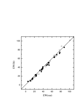
Figure 1: Comparison of solar EW measured in this study with those from the literature (Edvardsson et al edv93 (1993) – filled circles, Reddy et al red02 (2002) – open circles)

3 Atmospheric parameters

In order to perform reliable abundance determinations, it is crucial to derive accurate stellar parameters, especially effective temperatures $\mathrm{T_{eff}}$ . V-K or IR flux methods are often advocated as the best (Asplund asp03 (2003)) but require homogeneous infrared observations which are not available for all stars. Recently our group has improved the line-depth ratio technique pioneered by Gray (1994), leading to high precision $\mathrm{T_{eff}}$ for most of our program stars (Kovtyukh et al 2003). This method, relying on ratios of the measured central depths of lines having very different functional dependences on $\mathrm{T_{eff}}$ , is independent of interstellar reddening and takes into account the individual characteristics of the star’s atmosphere. Briefly, a set of 105 relations was obtained, the mean random error of a single calibration being 60–70 K (40–45 K in the most and 90–95 K in the least accurate cases). The use of $\sim$70–100 calibrations per spectrum reduced the uncertainty to 5–7 K. These 105 relations were obtained from 92 lines, 45 with low ($\chi<$2.77 eV) and 47 with high ($\chi>$4.08 eV) excitation potentials, calibrated from 45 reference stars in common with Alonso et al (AAMR96 (1996)), Blackwell & Lynas-Gray (BLG98 (1998)) and di Benedetto (dB98 (1998)). The zero-point of the temperature scale was directly adjusted to the Sun, based on 11 solar reflection spectra taken with ELODIE, leading to the uncertainty in the zero-point of about 1K. Judging by the small scatter in our final calibrations and $\mathrm{T_{eff}}$ , the selected combinations are only weakly sensitive to effects like rotation, micro- and macroturbulence, non-LTE and other. The application range of the line-depth method is $-0.5<$$\mathrm{[Fe/H]}$ $<+0.5$.

For the most metal-poor stars, $\mathrm{T_{eff}}$ was determined earlier (Mishenina & Kovthyukh mk01 (2001)). The H_α line-wing fitting was used for stars studed in this work. None of the stars from Mishenina & Kovthyukh (2001) had their temperature measured by line depth ratio because they are too metal poor. In order to testify that the temperature scales adopted in Mishenina & Kovthyukh (mk01 (2001)) and Kovtyukh et al (2003) are consistent, we show in Fig. 2 our adopted temperatures versus those estimated by Alonso et al (AAMR96 (1996)), Blackwell & Lynas-Gray (BLG98 (1998)) and di Benedetto (dB98 (1998)). Our temperature scale is slightly hotter than their by $\sim 20-30$K, as mentioned in Kovtyukh et al (2003), but the dispersion is satisfactory ($\sim 80$K, Tab. 1). We have checked the 2 outliers HD101177 and HD165341. We are certain that Alonso et al’s temperature for HD101177 (5483K) is in error because recently Heiter & Luck (heit03 (2003)) determined a temperature of 6000K similar to ours (5932K), a value confirmed by the H_α profile. HD165341 is a variable, active, rotating spectroscopic binary rending its photometric measurements suspicious. On the basis of IR photometry, Alonso et al (AAMR96 (1996)), Blackwell & Lynas-Gray (BLG98 (1998)) and di Benedetto (dB98 (1998)) determined respectively 4978K, 4983K, 4937K. Our determination of 5314K agrees well with that of Zboril & Byrne (zbo98 (1998)) who find $\mathrm{T_{eff}}$ =5260K.

Figure 2: Comparison of our adopted temperatures with those estimated by Alonso et al (AAMR96 (1996)), Blackwell & Lynas-Gray (BLG98 (1998)) and di Benedetto (dB98 (1998)). Crosses indicate stars with $\mathrm{[Fe/H]}$ $<$-0.5. The two outliers HD101177 and HD165341 are discussed in the text. HD165341 was measured by Alonso, Blackwell and Di Benedetto, that is why there are 3 points for the same star.

Table 1: Mean difference and standard deviation between our temperatures and those estimated by Alonso et al (AAMR96 (1996)), Blackwell & Lynas-Gray (BLG98 (1998)) and di Benedetto (dB98 (1998)) for $\sim$ 40 stars in common.

Reference	N	$\Delta T_{\rm eff}(K)$	$\sigma(K)$
Alonso et al (AAMR96 (1996))	43	31	84
Blackwell & Lynas-Gray (BLG98 (1998))	41	29	84
di Benedetto (dB98 (1998))	41	23	78

Finally, Fig. 3 shows a general lack of correlation between the Fe and Mg abundances and $\mathrm{T_{eff}}$ that testifies to a correct choice of the effective temperatures.

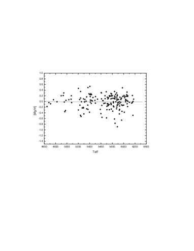
Figure 3: Abundances of Fe and Mg vs $\mathrm{T_{eff}}$

The two most commonly used techniques to determine surface gravities are the ionization balance of neutral and ionized species and the fundamental relation which expresses the gravity as a function of mass, temperature and bolometric absolute magnitude deduced from parallaxe. For the latter method, stellar masses can be estimated from evolutionary tracks, but metallicities and eventual $\alpha$-enhancement have to be known first. We therefore choosed to derive $\log\mathrm{g}$ from ionization balance, a method which might be affected by NLTE effects. However, a detailed study of surface gravities derived by different procedures was preformed by Allende Prieto et al (all99 (1999)) who concluded that astrometric and spectroscopic (iron ionization balance) gravities were in good agreement in the metallicity range $-1.0<$$\mathrm{[Fe/H]}$ $<+0.3$. We compared our adopted surface gravities to those determined astrometrically by Allende Prieto et al (all99 (1999)) and obtain a mean difference and standard deviation of -0.01 and 0.15 respectively for 39 stars in common. This is consistent with an accuracy of 0.1 dex on our estimated spectroscopic gravities. As an additional criterion of the reliable choice of $\log\mathrm{g}$ we used the wings-fitting for the MgIb lines. For all stars the difference does not exceed 0.2 dex (such difference was detected only for a few program stars).

Microturbulent velocities $V_{\rm t}$ were determined by forcing the abundances determined from individual FeI lines to be independent of equivalent width. Starting with $V_{\rm t}$=1.1 $\mathrm{\,km\,s}^{-1}$ , we varied it until abundances computed for FeI lines (20 mÅ$<$ EW $<$ 150 mÅ) and plotted as a function of EW-s showed a zero slope. The precision of the microturbulent velocity determination is 0.2 $\mathrm{\,km\,s}^{-1}$ .

The abundance of iron relative to solar one $\mathrm{[Fe/H]}$ =log(Fe/H)_∗ – log(Fe/H)_⊙ was used as the metallicity parameter of a star and was obtained from FeI lines.

The adopted parameters of the target stars are given in Table 8. To check the adopted model atmosphere parameters, we compared our values with those derived by Edvardsson et al (edv93 (1993)), Gratton et al (grat96 (1996)) Fuhrmann (fuhr98 (1998)), Chen et al (chen00 (2000)) and Fulbright (ful00 (2000)). The mean differences (other – us) and standard deviations are given in Table 2. On the whole, the agreement is rougly good.

Table 2: Number of stars in common, mean difference and standard deviation of parameter comparison with 5 other studies.

N	$\Delta T_{\rm eff}$	$\sigma$	$\Delta\log\,g$	$\sigma$	$\Delta$$\mathrm{[Fe/H]}$	$\sigma$	Ref∗
37	–2	78	0.03	0.17	–0.07	0.08	1
39	–28	82	0.04	0.22	–0.04	0.10	2
18	10	75	0.04	0.15	–0.01	0.09	3
17	–99	56	–0.06	0.13	–0.08	0.06	4
12	–15	74	0.05	0.16	0.04	0.09	5

• 1 – Edvardsson et al (1993); 2 – Gratton et al (1996); 3 – Fuhrmann (1998); 4 – Chen et al (2000); 5 – Fulbright (2000);

4 Abundance determination

4.1 Fe, Si, Ni abundances

Fe, Si, Ni abundances were determined from an LTE analysis of equivalent widths using the WIDTH9 code and the atmosphere models by Kurucz (kurucz93 (1993)). Appropriate models for each star were derived by means of standard interpolation through $\mathrm{T_{eff}}$ and $\log\mathrm{g}$ . The model metallicities were taken with an accuracy of $\pm$0.25 dex around the TGMET first guess. Abundances of the investigated elements Fe, Si, Ni were carried out from a differential analysis relative to the Sun. Solar abundances of Fe, Si and Ni were calculated with our solar EWs and the oscillator strengths log gf from Kovtyukh & Andrievsky (1999), who derived log gf for 565 lines of the 27 chemical elements using solar spectra. We determined : log A(Fe) = 7.55, log A(Si) = 7.55, log A(Ni) = 6.25, where log(H) = 12 (according to Grevesse & Sauval (1998) log A(Fe) = 7.50, log A(Si) = 7.55, log A(Mg) = 7.58, log A(Ni) = 6.25).

Depending on authors, the solar iron abundance varies from 7.44 to 7.64 (Asplund et al 2000; Blackwell et al 1995; Gehren et al 2000a; Grevesse & Sauval 1998; Shchukina & Bueno 2001, etc). This disagreement is caused by several factors: the systems of oscillators strengths, the models of solar atmosphere (empirical, hydrodynamical, LTE or NLTE assumptions), the solar spectrum LTE or NLTE synthesis etc. Using laboratory log gf, Blackwell et al (1995) have obtained a solar iron abundance of 7.64. From calculated and laboratory log gf, Gehren (2001a) found an abundance 7.50 and 7.56 from Fe II lines, and 7.47 and 7.56 from Fe I lines. The detailed hydrodynamical models of the Sun result in the solar value of iron abundance of 7.44 (Fe I lines) and 7.45 (Fe II lines) (Asplund et al asplundet00 (2000) 2000). In the same time of the meteoretic value of the iron abundance is 7.50 (Grevesse & Sauval 1998). The same value was found for the solar atmosphere by Shchukina & Bueno (2001) using the NLTE approximation and hydrodynamical solar model. The solar silicon abundance obtained within the framework of the hydrodynamical models (Asplund 2000) is sligtly lower (7.51) than the meteoric silicon abundance (7.55) (Grevesse & Sauval 1998). To reduce the influence of the used systems of oscillators strengths, atmosphere models and instrumental errors we used a differential method of abundance determination.

The list of Fe, Si and Ni lines, atomic parameters and solar EW are given in Table 3. Relative abundances of Fe, Si and Ni are given in Table 8.

Table 3: List of Fe, Si and Ni lines, atomic parameters and solar EW. Only available at the CDS

4.2 NLTE calculations for Mg

The determination of Mg abundance was carried out through detailed NLTE calculations using equivalent widths of 4 lines ($\lambda$ $\lambda$ 4730, 5711, 6318, 6319 Å) and profiles of 5 lines ($\lambda$ $\lambda$ 4571, 4703, 5172, 5183, 5528 Å).

NLTE abundances of Mg were determined with the help of a modified version of the MULTI code of Carlsson (Carl (1986)) described in Korotin et al. (1999a 1999b ). We have included in the code opacity sources from the ATLAS9 program (Kurucz Kur2 (1992)). This enables a much more accurate calculation of the continuum opacity and intensity distribution in the UV region which is extremely important in the correct determination of the radiative rates of $b-f$ transitions. For $b-b$ transitions include only continuum opacity and for $b-f$ transitions include continuum both opacities and line opacities from ATLAS9. A simultaneous solution of the radiative transfer and statistical equilibrium equations has been performed in the approximation of complete frequency redistribution for all lines.

We employed the model of magnesium atom consisting of 97 levels: 84 levels of Mg i, 12 levels of Mg ii and a ground state of Mg iii. They were selected from works of Martin & Zalubas (MarZal (1980)) and Biemont & Brault (BiBr (1986)). A detailed structure of the multiplets was ignored and each $LS$ multiplet was considered as a single term. The fine structure was taken into account only for a level $3s3p^{3}P^{0}$, since it is closely connected to the most important transitions in magnesium atom ( $\lambda$ $\lambda$ 2778 – 2782ÅÅ , 3829 – 3838 ÅÅ , 5167 Å , 5172 Å ).

Within the described system of the magnesium atom levels, we considered the radiative transitions between the first 59 levels of Mg i and ground level of Mg ii. Transitions between the rest levels were not taken into account and they were used only in the equations of particle number conservation.

Only transitions with $\lambda<100000$ Å  were selected for the analysis. All 424 $b-b$ transitions were included in the linearization procedure.

Grotrian diagram for the MgI are displayed in Fig. 4.

Figure 4: Grotrian diagram for MgI. Displayed are the radiative transitions treated explicity in the non-LTE calculations

Photoionization cross-sections were mainly taken from the Opacity Project (Yan et al Yan (1987)) keeping a detailed structure of their frequency dependence, including resonances. For some important $b-f$ transitions, the cross-section structure is extremely complicated making it difficult to describe it using only simple approximations like $\sim\nu^{-3}$.

Oscillator strengths were selected from the extensive compilative catalogue by Hirata & Horaguchi (Hir (1994)). Some information was obtained through the Opacity Project. As we ignored a multiple structure of all the levels, the oscillator strengths for each averaged transition were calculated as $f=\frac{\sum g_{i}f_{i}}{\sum g_{i}}$.

After the combined solution of radiative transfer and statistical equilibrium equations, the averaged levels have been split with respect to multiplet structure, then level populations were redistributed proportionally to the statistical weights of the corresponding sublevels and finally the lines of the interest were studied.

Electron impact ionization was described using Seaton’s formula (Seaton Seaton (1962)). Collision rate between ground level Mg i and ground level of Mg ii were approximated by use of the fits from Voronov (Voronov (1997)). For electron impact excitation for all allowed $b-b$ transitions we used the van Regemorter (Regem (1962)) formula. Collisional rates for the forbidden transitions were calculated by using the semiempirical formula (Allen Allen (1973)), with a collisional force of = 1.

Inelastic collisions with hydrogen may play a significant role in the atmospheres of cool stars. We took into account this effect with the help of Drawin’s formulas (Drawin (1968)) offered Steenbock & Holweger (Steen (1984)), with a correction factor of 1/3. Nevertheless, as it was shown in our test calculation, the influence of such collisions is negligible for the stars considered in our paper. In particular, the variation of the correction factor from 0 to 1 results in a change of the equivalent width less than 0.5%.

For all the transitions we also took into account such broadening parameters of lines as radiative damping, Stark effect, van der Waals damping and microturbulent velocity. For temperatures, considered by us, the influence of Stark effect is small.

The main influence on the profile was exerted by van der Waals broadening. The Unsöld’s (Uns (1955)) formula which is widely used to allow for this effect, is known to yield somewhat understimated coefficients C₆. To refine these coefficients, we conducted a special comparison of the observed and calculated line profiles in solar spectrum using method Shimanskaya, Mashonkina & Sakhibullin (SMS (2000)). The Solar Flux Atlas of Kurucz et al. (Kur1 (1984)) and Kurucz’s model of the solar atmosphere (Kur2 (1992)) were used. To take into account the chromospheric growth of temperature, this model was completed by a model of the solar chromosphere from work of Maltby et al.(Maltb (1986)). Nevertheless, the influence of a chromosphere on the equivalent width of considered lines was insignificant (less than 1%).

The corrections $\Delta$log C₆ to the classic Unsöld (1955) collisional damping constant derived from solar line wing fitting are given in Table 4. These values are comparable for common lines with results obtained in the paper of Shimanskaya, Mashonkina & Sakhibullin (SMS (2000)). Similar values were obtained by Barklem, Piskunov & O’Mara (BPO (2000)). For example, their correction factors for the lines $\lambda\lambda$ 5172, 5183 ÅÅ  are $\Delta$log C₆=0.85. Oscillator strengths for observed lines were selected from the compilative catalogue by Hirata & Horaguchi (Hir (1994)).

Table 4: Atomic data for the Mg lines

Lambda	$\chi$ (eV)	log gf	$\Delta$C6	$\Delta$C6 (Barklem et al 2000)
4571.10	0.00	-5.79	1.72
4702.99	4.35	-0.52	0.74	1.33
4730.03	4.35	-2.32	1.75
5172.68	2.71	-0.38	0.74	0.85
5183.60	2.71	-0.16	0.72	0.85
5528.40	4.35	-0.49	0.44	0.95
5711.09	4.35	-1.72	0.60
6318.72	5.11	-1.97	1.19
6319.24	5.11	-2.18	1.19
6319.49	5.11	-2.61	1.19

The estimates obtained from the NLTE profile analysis of the MgI lines in the solar spectrum give the solar magnesium content (Mg/H)=7.57$\pm$0.02 which agrees well with the determination of Grevesse & Sauval (Grev98 (1998)) and Shimanskaya, Mashonkina & Sakhibullin (SMS (2000)), who derived (Mg/H)=7.58.

The comparison the NLTE profiles with those observed are presented in Fig. 5. NLTE abundances of Mg are given in Table 8.

The NLTE effects for the used lines appeared to be very small (less than 0.05 dex). The similar results were obtained in Shimanskaya, Mashonkina & Sakhibullin (SMS (2000)).

Figure 5: Comparison of synthetic NLTE profiles (continuous line) of the MgI lines to the observed spectrum of HD224930 (dots)

5 Error analysis

Average standard deviations of abundances obtained from 72 - 265 lines of Fe I (the number of used lines differs from star to star), 11 - 24 lines of Si I and 12 - 17 lines of Ni I are 0.10, 0.08 and 0.08 respectively. Final errors in abundances result mainly from errors in the choice of parameters of the model atmospheres and in equivalent width measurements (gaussian fitting, placement of the continuum) in the case of Fe, Si, and Ni or fitting a synthetic spectrum in the case of Mg. Table 5 lists the errors obtained when changing the atmospheric parameters by $\Delta$$\mathrm{T_{eff}}$ = -100 K; $\Delta$$\log\mathrm{g}$ =+0.2; $\Delta$ V_t=+0.2 $\mathrm{\,km\,s}^{-1}$ ; $\Delta$$\mathrm{[Fe/H]}$ =$\pm$0.25 and by assuming an uncertainty of $\pm$2 mÅ  in the EW. These values were adopted taking into account the intrinsic accuracy of the atmospheric parameter determination, the processing of the spectra and the comparison of our parameter definition with those of other authors. This test has been performed for 3 stars with different characteristics.

As seen in Table 5, the total uncertainty reaches 0.12 dex for iron abundance determined from II species and 0.10 dex in the case of I species. The standard deviation obtained by comparing our $\mathrm{[Fe/H]}$ determinations to those obtained by other authors (Table 2) shows that we are consistent with them at a level lower than 0.10 dex.

Table 5: Effects of uncertainties of model parameters and EW measurements on the derived abundances

	HD004614		5965/4.4/1.1/–0.24
El	$\mathrm{T_{eff}}$	$\log\mathrm{g}$	Vt	EW	$\mathrm{[Fe/H]}$	Total
FeI	0.07	0.02	0.04	0.04	0.00	0.09
FeII	–0.02	–0.08	0.02	0.04	0.03	0.10
MgI	0.05	0.02	0.02	0.03	0.00	0.06
SiI	0.02	0.01	0.02	0.03	0.01	0.05
NiI	0.07	0.00	0.03	0.04	0.00	0.09
	HD022879		5972/4.5/1.1/–0.77
FeI	0.05	0.02	0.02	0.08	0.00	0.10
FeII	–0.01	–0.09	0.01	0.07	0.02	0.12
MgI	0.07	0.03	0.02	0.04	0.00	0.09
SiI	0.02	–0.01	0.00	0.05	0.00	0.05
NiI	0.07	0.01	0.01	0.06	0.00	0.09
	HD117176		5611/4.0/1.0/-0.03
FeI	0.07	0.03	0.04	0.04	0.01	0.10
FeII	–0.04	–0.10	0.02	0.04	0.04	0.12
MgI	0.06	0.03	0.03	0.03	0.00	0.08
SiI	0.01	–0.01	0.02	0.03	0.02	0.05
NiI	0.06	0.00	0.03	0.04	0.01	0.08

• – $\Delta$$\mathrm{T_{eff}}$ = -100 K;

• – $\Delta$$\log\mathrm{g}$ = +0.2;

• – $\Delta$V_t=+0.2 $\mathrm{\,km\,s}^{-1}$ ;

• – $\Delta$$\mathrm{[Fe/H]}$ = –0.25 dex;

• – $\Delta$EW= $\pm$ 2mÅ ;

• – Total error.

For Mg, Si and Ni, the total uncertainty due to parameter and EW errors is 0.08 dex, 0.05 dex and 0.09 dex respectively. We have also compared our Mg, Si and Ni abundances with those determined by other authors. For [Mg/H], we have carried out the comparison with Idiart & Thévenin (2000) and Gratton et al (2003) who have also used the NLTE approach. Our [Si/Fe] and [Ni/Fe] determinations have been compared to those of Edvardsson et al (edv93 (1993)), Reddy et al (red02 (2002)) and Chen et al (2000). The results of comparisons are listed in Table 6. The mean differences are lower than 0.05 and the standard deviations lower than 0.1 dex for all elements proving the good consistency of our study with previous works relying on similar methods.

Table 6: Abundance [Mg/H], [Si/Fe], [Ni/Fe] comparison with other authors

N	$\Delta_{Mg}$	$\sigma$	$\Delta_{Si}$	$\sigma$	$\Delta_{Ni}$	$\sigma$	Ref∗
18	0.03	0.09					1
10	0.04	0.09					2
37			–0.05	0.05	0.01	0.05	3
17			–0.04	0.05	0.02	0.03	4
5			0.01	0.08	–0.05	0.09	5

• 1 – Idiard & Thévenin (2000); 2 – Gratton et al (2003); 3 – Edvardsson et al (1993); 4 – Chen et al (2000); 5 – Reddy et al (2003)

6 Stellar kinematics, metallicity, elemental abundances

All the selected stars are bright and nearby enough to have parallaxes and proper motions measured by Hipparcos (ESA ESA97 (1997)). These astrometric quantities have been combined with radial velocties measured on the ELODIE spectra by cross-correlation (with an accuracy better than 100 $\mathrm{m\,s}^{-1}$) to compute the 3 components (U,V,W) of the spatial velocities with respect to the Sun. Combining the measurement errors on parallaxes, proper motions and radial velocities, the resulting errors on velocities are of the order of 1 $\mathrm{\,km\,s}^{-1}$ .

Our first concern was to analyse the content of our sample in terms of stellar populations. As we were interested in the characterization of abundance patterns in the thin disk and the thick disk, we have selected our sample to span the metallicity range $-1.0<$$\mathrm{[Fe/H]}$ $<+0.3$ in order to define 2 subsamples representative of these two populations. A discrimination of thin disk and thick disk stars is possible using the fact that the two disks are known to be distinct by their spatial distribution and local density, and by their velocity, metallicity and age distributions. However we have performed this classification with a pure kinematical appoach because velocity distributions are the best constrained from observations reported in the literature. If the thin disk velocity distribution is well known thanks to Hipparcos data, authors do not yet agree on the properties of the thick disk. A review of the current knowledge of the thick disk is given in Norris (N99 (1999)). There is still a controversy between the adherents of a flat and dense thick disk, with typical scale height of 800 pc and local relative density of 6-7% (Reylé & Robin RR01 (2001)) to 15% (Soubiran et al soub03 (2003)), and the adherents of a thick disk with a higher scale height, typically 1300 pc and a lower local relative density, of the order of 2% (Reid & Majewski RM93 (1993)). Velocity dispersions are generally found to span typical values between 30 and 50 $\mathrm{\,km\,s}^{-1}$ , with an asymmetric drift between -20 and -80 $\mathrm{\,km\,s}^{-1}$ . Recently, Soubiran et al (soub03 (2003)) determined the kinematical parameters of the thick disk and the thick disk from an unbiased sample of clump giants. These values, listed in Tab. 7, are used in the present study.

Table 7: Kinematical parameters adopted for the thin disk and the thick disk from Soubiran et al (soub03 (2003))

	thin disk	thick disk
$\rm V_{lag}$ ($\mathrm{\,km\,s}^{-1}$ )	-15	-51
$\sigma_{U}$ ($\mathrm{\,km\,s}^{-1}$ )	39	63
$\sigma_{V}$ ($\mathrm{\,km\,s}^{-1}$ )	20	39
$\sigma_{W}$ ($\mathrm{\,km\,s}^{-1}$ )	20	39

The metallicity distributions of the thin and thick disks are also matter of debate. Recent thick disk metallicity determinations quoted mean values from -0.36 (Bell bel96 (1996)) to -0.70 (Robin et al rob96 (1996), Gilmore et al gil95 (1995)), passing by -0.48 (Soubiran et al soub03 (2003)). Morrison et al (MFF90 (1990)) brought to the fore low-metallicity stars $(-1.6<$$\mathrm{[Fe/H]}$ $<-1.0)$ with disk-like kinematics. Chiba & Beers (CB00 (2000)) estimate that 30% of the stars with $-1.6<$$\mathrm{[Fe/H]}$ $<-1.0$ belong to the thick disk population. Similarly, Bensby et al (ben03 (2003)) found in their sample stars with super-solar metallicities and thick disk kinematics. It remains unclear whether these extreme populations are separate from the thick disk or their metal-weak and metal-rich tails. Moreover, due to the great overlap of the thin disk and thick disk distributions, it is very difficult to estimate where the transition occurs. Authors involved in the study of metallicity distributions are often concerned with the chemical evolution of the Galaxy and generally do not attempt to separate the thin and thick disks but rather consider the thick disk as an integral part of the disk. It was the case for instance in the work of Edvardsson et al (edv93 (1993)) on the age - metallicity relation. Haywood (H01 (2001)) performed a revision of the solar neighbourhood metallicity distribution and concluded that it peaks at $\mathrm{[Fe/H]}$ =0 and that only 4% of the nearby stars have $\mathrm{[Fe/H]}$ $<-0.50$. These considerations made us think that the selection of thin disk and thick disk stars on a pure kinematical criterion would be more reliable.

Fig. 6 shows the distribution of the sample in the plane metallicity - W velocity. It is clear from this plot that a transition occurs at $\mathrm{[Fe/H]}$ $\sim$ -0.30 : above this value we measure a dispersion of the W velocities of 16 $\mathrm{\,km\,s}^{-1}$ while below this value the dispersion is 38 $\mathrm{\,km\,s}^{-1}$ . These values are typical of the thin disk and the thick disk respectively (see Tab 7). They are related to the different scale heights of the two populations and testify that our sample is indeed a mixture of thin and thick disk stars.

Figure 6: Distribution of the 174 stars in the plane metallicity - W velocity.

In order to compute the probability of each star to belong to the thin disk or the thick disk on the basis of its spatial velocity, we need to know the kinematical parameters of the two disks and their proportion in our sample. The kinematical parameters are listed in Tab. 7, but the proportions in our sample are of course different of the real proportion in the solar neibourhood because our selection in the range $-1<$$\mathrm{[Fe/H]}$ $<+0.3$ is supposed to have increased the number of thick disk stars comparatively to their relative density in the solar neighbourhood (2% to 15%). Moreover the ELODIE library was build from various observing programs which may have biased its content and consequently our sample.

To estimate the proportion of thin and thick disk stars in our sample, we have applied an algorithm of deconvolution of multivariate gaussian distributions, on (U,V,W) velocities. This algorithm, SEM (Celeux & Diebolt CD86 (1986)), solves iteratively the maximum likelihood equations, with a stochastic step, with no a priori information on the mixture of the gaussian distributions. The results are unambiguous, our sample is consistent with a mixture of 2 gaussian populations with parameters very similar to those listed in Tab. 7, but with relative densities of 75% and 25% respectively for the thin disk and the thick disk. Accordingly, we have computed the probability of each star, with a measured velocity (U,V,W), to belong to the thin disk ($Pr_{1}$) and to the thick disk ($Pr_{2}$) :

$$Pr_{1}=p_{1}{F_{1}\over F},\,\,Pr_{2}=p_{2}{F_{2}\over F}$$

$$F_{i}={1\over{\sqrt{2\pi}^{3}\sigma_{U_{i}}\sigma_{V_{i}}\sigma_{W_{i}}}}\exp{-0.5[{{U\over\sigma_{U_{i}}^{2}}+{(V-V_{i})\over\sigma_{V_{i}}^{2}}+{W\over\sigma_{W_{i}}^{2}}}]}$$

$$F=p_{1}F_{1}+p_{2}F_{2}$$

where $p_{1}=0.75,p_{2}=0.25$ are the relative densities of the 2 populations in our sample and $V_{i},\sigma_{U_{i}},\sigma_{V_{i}},\sigma_{W_{i}},i=1,2$ are the kinematical parameters of the thin and thick disks listed in Table 7.

From these probabilities we have selected two subsamples kinematically representative of each population in order to highlight their respective properties. Putting the limit at $Pr_{i}>80$% ensures a minimal contamination of each subsample by the other population. The thin disk subsample includes 109 stars whereas the thick disk subsample include 30 stars. In the figures, unclassified stars are represented by small dots, thick disk stars by larger black dots, thin disk stars by open dots. The only halo star of the sample, HD194598 ($\mathrm{[Fe/H]}$ =-1.21, V=-276.40 $\mathrm{\,km\,s}^{-1}$ ) is not represented in the plots for a better clarity.

Fig. 7, 8 and 9 show the trend of the abundances of Mg, Si and Ni as a function of $\mathrm{[Fe/H]}$ . It can be seen that :

• there are a few thin disk stars with $\mathrm{[Fe/H]}$ $<-0.30$

• metal poor stars ($\mathrm{[Fe/H]}$ $<-0.60$) are all enriched in Mg and Si ($\mathrm{[Mg/Fe]}$ $>+0.20$, $\mathrm{[Si/Fe]}$ $>+0.15$)

• on the contrary at solar metallicity, the enrichment of Mg and Si does not exceed +0.20

• at a given metallicity thick disk stars have higher $\mathrm{[Mg/Fe]}$ on average than thin disk stars

• the dispersion of $\mathrm{[Si/Fe]}$ is remarkably small for $\mathrm{[Fe/H]}$ $>-0.30$ but quite high at lower metallicity

• $\mathrm{[Mg/Fe]}$ and $\mathrm{[Si/Fe]}$ decline with metallicity from about +0.40,+0.35 to 0.0, +0.08 respectively

• there are stars with thick disk kinematics at solar metallicities, their abundance trends follow the thin disk

• a rise and upturn is visible for $\mathrm{[Ni/Fe]}$ for $\mathrm{[Fe/H]}$ $>0$

All these features are in very good agreement with those described in Bensby et al (ben03 (2003)).

Figure 7: $\mathrm{[Mg/Fe]}$ vs $\mathrm{[Fe/H]}$ for the whole sample. Black dots indicate thick disk stars, open dots thin disk stars, small dots represent the unclassified stars.

Figure 8: Same as Fig. 7 for Si.

Figure 9: Same as Fig. 7 for Ni.

Fig. 10 represents the correlation between Mg and Si relative to iron. Mg and Si are $\alpha$ elements which are supposed to be mainly produced in SNII. It can be seen in this plot that a transition occurs at $\mathrm{[Mg/Fe]}$ $\simeq+0.2$. Stars with $\mathrm{[Mg/Fe]}$ $<+0.2$ have a mean abundance of $\mathrm{[Si/Fe]}$ =+0.08 with a very low dispersion of $\pm 0.03$, lower than our error estimates. $\mathrm{[Mg/Fe]}$ is more dispersed ($\pm 0.06$) around the mean of $\mathrm{[Mg/Fe]}$ =+0.05. For stars with $\mathrm{[Mg/Fe]}$ $>+0.2$ the distribution is consistent with a linear correlation : $\mathrm{[Si/Fe]}$ =0.7$\mathrm{[Mg/Fe]}$ +0.06 (rms=0.06).

Figure 10: Correlation between $\mathrm{[Mg/Fe]}$ and $\mathrm{[Si/Fe]}$

7 Discussion

7.1 Stars with thick disk kinematics and thin disk metallicity

A remarkable feature in the Fig. 7 to 10 is the behavior of stars with thick disk kinematics and thin disk metallicity. They follow exactly the chemical trend of the thin disk. This led us to wonder if these stars were real thick disk stars. According to the W vs $\mathrm{[Fe/H]}$ distribution shown in Fig. 6, metal-rich stars are expected to have a smaller scale height than metal poor stars. To have confirmation, we have computed the orbital parameters of our stars, by integrating the equations of motion in the galactic model of Allen & Santillan (allsan91 (1991)) over an age of 8 Gyr. The adopted velocity of the Sun with respect to the LSR is (9, 5, 6) $\mathrm{\,km\,s}^{-1}$ , the solar galactocentric distance ${\mathrm{R}}_{\odot}=8.5$ kpc and circular velocity ${\mathrm{V}_{lsr}}=220$ $\mathrm{\,km\,s}^{-1}$ . Table 8 lists the spatial velocities and the parameters of the orbits : apogalactic and perigalactic distances ($\mathrm{R_{min},R_{max}}$), the maximum distance from the plane ($\mathrm{Z_{max}}$ ) and eccentricity ($e$). The distribution of $\mathrm{Z_{max}}$ vs $\mathrm{[Fe/H]}$ in Fig. 11 confirms the small scale height of stars with thick disk kinematics and solar metallicity, ruling them out of the thick disk. They have been classified into the thick disk because of they have a large eccentricity, but they have a scale height which is typical of the thin disk. Thus the origin of these stars cannot be in the thick disk neither in the local thin disk despite the same chemical behaviour. The origin of these stars has to be found elsewhere.The only ambiguous star, HD190360 having $\mathrm{[Fe/H]}$ =+0.12 and $\mathrm{Z_{max}}$ =1 kpc, appears as an outlier in the distribution. This star is discussed farther.

Figure 11: The maximum distance to the plane of orbits, $\mathrm{Z_{max}}$ , versus $\mathrm{[Fe/H]}$

Among the 8 stars that verify $\mathrm{Pr}_{2}>80$% and $\mathrm{[Fe/H]}$ $>-0.30$, HD030562, HD139323, HD139341 are K dwarfs with very similar velocities and metallicities (Tab. 8, $+0.18\leq$$\mathrm{[Fe/H]}$ $\leq+0.21$. HD030562 has been identified to be part of the HR 1614 moving group by Feltzing & Holmberg (FH00 (2000)). It is very likely that we have discovered 2 new candidates of this moving group whose age is estimated to be 2 Gyr. The origin of this group is however unknown.

HD010145, HD135204, HD152391 have $|U|>80$ $\mathrm{\,km\,s}^{-1}$ . An hypothesis is that they have been thrown out from the inner disk by the galactic bar. The over density of metal-rich stars with excentric orbits confined near the plane have have been interpreted as the signature of the galactic bar in the solar neighbourhood by Raboud et al (rab98 (1998)) for instance.

Bensby et al (ben03 (2003)) have also found several stars with thick disk kinematics and thin disk metallicity on the basis of a similar probability calculation than ours, but using the ratio of $\mathrm{Pr_{2}}$ to $\mathrm{Pr_{1}}$. If in our case these stars have a clearly a flatter distribution than the thick disk, it was not mentioned in Bensby et al’s study. As it is important to demonstrate if they belong or not to the thick disk we have calculated the orbits of their stars and classified them with the same criterion as ours ($\mathrm{Pr_{i}}>80$%). The distribution of $\mathrm{Z_{max}}$ versus $\mathrm{[Fe/H]}$ is shown on Fig. 12. Globally their distribution is similar to ours despite their sample is much smaller. There is a sudden rise in $\mathrm{Z_{max}}$ at $\mathrm{[Fe/H]}$ $<-0.3$. They have also 3 outliers with solar metallicities and $\mathrm{Z_{max}}$ $\sim 1$ kpc, HD190360 being in common with us. The five other stars with thick disk kinematics and $\mathrm{[Fe/H]}$ $>-0.30$ have a low scale height typical of the thin disk in agreement with our findings. The question wether HD190360, HD003648 and HD145148 are really part of the thick disk is an open question because they appear as outliers in the distribution of kinematics vs metallicity. It is only with complete samples with no kinematical bias that the relation of such stars with the thick disk will be clarified.

Figure 12: The maximum distance to the plane of orbits, $\mathrm{Z_{max}}$ , versus $\mathrm{[Fe/H]}$ for Bensby et al’s sample. The classification thin disk / thick disk is the same as ours ($\mathrm{Pr}_{i}>80$%).

7.2 The thin disk

Several thin disk stars are found at low metallicity, down to $\mathrm{[Fe/H]}$ $=-0.80$. Several previous studies have also established the existence of such stars, however the exact contribution of metal-poor stars to the thin disk is difficult to evaluate from uncomplete samples. Reddy et al (red02 (2002)) have found in their samples a significant number of stars with $\mathrm{[Fe/H]}$ $<-0.40$ that they identify as belonging to the thin disk. They have analysed 181 FG dwarfs, a sample size similar to ours. Their sample spans the metallicity interval –0.70 to +0.15, with a peak at $\mathrm{[Fe/H]}$ =–0.40. Only 3 stars were identified as belonging to the thick disk, based on the criterion $\mathrm{[Mg/Fe]}$ $>+0.20$, all the other stars being identified as thin disk stars. The peak at $\mathrm{[Fe/H]}$ =–0.40 shows clearly that they have favoured in some way the metal-poor tail of the thin disk. Unfortunatly their selection criteria are not described. On the contrary, the way Chen et al (chen00 (2000)) have favoured metal-poor thin disk stars in their sample is very clear : they have selected equal number of stars in every metallicity interval of 0.1 dex in the range $-1.0<$$\mathrm{[Fe/H]}$ $<+0.3$. According to the low density of the thick disk in the solar neighbourhood, thin disk stars are still dominating at moderatly low metallicity. Haywood (H01 (2001)) has very carefully taken into account the selection biases of his sample to study the metallicity distribution of the local disk but his metallicities are photometric and no special attention was paid to a kinematical distinction between the thin disk and the thick disk. Nevertheless he found, contrary to Wyse & Gilmore (WG95 (1995)), a low contribution of the thin disk at $\mathrm{[Fe/H]}$ $<-0.40$.

Our observations suggest that the distribution of $[\alpha/\mathrm{Fe}]$ in the thin disk is very narrow, specially for Si, at $\mathrm{[Fe/H]}$ $>-0.30$. On this point we are in perfect agreement with Reddy et al (red02 (2002)) and Bensby et al (ben03 (2003)). For the metal-rich part, we obtain as mean values and dispersions : $\mathrm{[Mg/Fe]}$ =+0.05, $\sigma_{\mathrm{[}Mg/Fe]}$=0.07, $\mathrm{[Si/Fe]}$ =+0.07, $\sigma_{\mathrm{[}Si/Fe]}$=0.03. Such a narrow chemical distribution implies that the stars formed from an homogeneous gas. At lower metallicity, the Mg enhancement is higher. However at a given metallicity the thin disk shows a lower Mg enhancement than the thick disk. The behaviour of Si is quite surprising, showing high dispersion, whereas Bensby et al (ben03 (2003)) find a similar behaviour than Mg. We notice also that the Sun would be slightly Si-poor as compared to the thin disk. However this offset stays within the error bars and might be related to the adopted zero point of our abundance scales. Many previous studies (Edvardsson et al edv93 (1993), Chen et al chen00 (2000), Reddy et al red02 (2002), Bensby et al ben03 (2003)) exhibit also a positive offset in $\mathrm{[Si/Fe]}$ of the thin disk.

A rise of $\mathrm{[Ni/Fe]}$ from $\sim$ –0.1 at $\mathrm{[Fe/H]}$ =-0.20 to $\sim$ +0.1 at $\mathrm{[Fe/H]}$ =+0.20 is visible in Fig. 9 as well as an upturn for the most metal rich star. A similar feature is also observed in Bensby et al (ben03 (2003)).

7.3 The thick disk

Having eliminated from the thick disk the 8 stars having high metallicity and a flat distribution (Sect. 7.1), we see from Figure 7 that $\mathrm{[Mg/Fe]}$ decreases from the halo value (+0.40) at $\mathrm{[Fe/H]}$ =-1.00 to +0.20 at $\mathrm{[Fe/H]}$ =-0.30. Si has the same behaviour, decreasing from +0.35 to +0.17, with one deviating star HD110897 having a lower enrichment in Si. These findings are nicely consistent with the trends found by Bensby et al (ben03 (2003)) that they interpreted as the signature of the chemical enrichment by SNIa. Feltzing et al (felt03 (2003)) claimed the existence of a ”knee” in the $[\alpha/\mathrm{Fe}]$ abundance trends tracing the beginning of the contribution of the SNIa. This ”knee” may also exist in our data, especially in $\mathrm{[Mg/Fe]}$ but the dispersion is too high to conclude. Definitively a larger sample of thick disk stars is necessary to clarify this point. Contrary to Bensby et al (ben03 (2003)) and Feltzing et al (felt03 (2003)), our data suggest that the metallicity distribution of the thick disk does not continue at solar metallicity. The trend of declining ehancement, which was also mentioned in Prochaska et al (pro00 (2000), has to be compared to the results of Fuhrmann (fuhr98 (1998)) and Gratton et al (grat00 (2000)) who found in the thick disk a constant overabundance of $\alpha$-elements with respect to iron, with a value similar to that of the halo. In Fuhrmann (fuhr98 (1998)), only thin disk stars exhibit a decrease of $\mathrm{[Mg/Fe]}$ with increasing $\mathrm{[Fe/H]}$ . We believe that we have been able to detect this trend, as Feltzing et al (felt03 (2003)) and Bensby et al (ben03 (2003)), because we have used a more precise criterion to isolate a sample a pure thick disk stars. We agree with most of the previous works that a discontinuity exists between the chemical distributions of the thin and thick disks. Our data suggest that the star formation in the thick disk stopped when the gas had the composition $\mathrm{[Fe/H]}$ =–0.3, $\mathrm{[Mg/Fe]}$ =+0.20, $\mathrm{[Si/Fe]}$ =+0.17.

The distribution of $\mathrm{Z_{max}}$ vs $\mathrm{[Fe/H]}$ (Fig. 11) does not exhibit a clear vertical gradient in the thick disk metallicity. We have searched for a vertical gradient in the $\alpha$-element abundances. Fig. 13 represents $\mathrm{Z_{max}}$ vs $[\alpha/\mathrm{Fe}]$ =0.5($\mathrm{[Mg/Fe]}$ +$\mathrm{[Si/Fe]}$ ) for the thick disk (Pr2¿0.80 and [Fe/H]¡-0.3). A gradient may exist, but should be confirmed with a larger sample. The existence of a vertical gradient would imply a significant timescale for the formation of the thick disk. This implication is also true if the decline of $\alpha$ enhancement is interpreted by the onset of SNIa.

Figure 13: A possible vertical gradient in [$\alpha$/Fe] in the thick disk ?

8 Summary and perspectives

We have investigated the chemical behaviour of the thin disk and the thick disk with a large sample of FGK dwarfs spanning the metallicity interval [-1.00 ; +0.30]. We have used an homogeneous set of high resolution, high S/N echelle spectra to derive abundances of Fe, Mg, Si and Ni with detailed NLTE calculations for Mg. All sources of errors have been analysed and we have compared our abundances with several studies taken in the literature, showing a good agreement. Orbits and space velocities were computed and used to estimate the probability of each star to belong to the thin disk and the thick disk, taking into account the selection bias that affects our local sample where the thick disk is overrepresented as compared to the solar neighbourhood. Our main findings concern the transition in kinematics and abundance trends which occurs at $\mathrm{[Fe/H]}$ $=-0.30$, the decline of $\alpha$ enhancement with increasing $\mathrm{[Fe/H]}$ in the thick disk, and the narrow distribution of Mg and Si in the thin disk. We have also observed several stars which cannot belong to the thin disk because of their large eccentricity, neither to the thick disk because of their low scale height. This population, perhaps coming from the inner disk due to a dynamical effect, has to be taken into account when studying the metallicity distributions of the stellar populations in the solar neighbourhood. Among these stars we have discovered two new candidates of the HR 1614 moving group.

Larger samples are necessary to confirm our findings on the thin disk and the thick disk. Unfortunatly thick disk stars are quite rare in the solar neighbourhood and the construction of a significant sample of local thick disk stars implies either a huge complete sample of disk stars, among which 2% to 15% of thick disk stars are expected, or the selection of such stars by kinematical or chemical criteria which bias the conclusions which can be drawn. A lot of observing material is available. In the public ELODIE library, there are hundreds of high quality spectra of FGK stars that have not been analysed yet. Most of these stars have accurate parallaxes and proper motions from Hipparcos and their radial velocities are also available. It is thus possible to compute their probability to belong to a given kinematical population. More difficult but necessary is to evaluate the biases which render the metal-poor and high velocity stars more represented in the library than in the solar neighbourhood, reflecting the interest of observers in this kind of stars. Another solution to avoid these biases is to observe the thick disk in situ that is at distances and galactic latitudes where it begins to dominate the thin disk in density. We are continuing such an observing program (Soubiran et al soub03 (2003)).

Detailed analysis of spectroscopic data is a tedious work that takes much time to measure equivalent widths, to fit profiles, to compute models etc… It is now absolutly necessary to develop automatic methods to take advantage of the huge amount of high quality data which is provided by the new generation of spectrographs. We have undertaken such work to continue our investigation of the correlation between elemental abundances and kinematics among galactic disk stars from larger, more distant and complete samples.

Table 8: Atmospheric parameters, abundances, 3D velocities with respect to the Sun, orbital parameters, probability to belong to the thin disk and the thick disk for the 174 program stars

HD	$\mathrm{T_{eff}}$	$\log\mathrm{g}$	$\mathrm{[Fe/H]}$	$\mathrm{[Mg/Fe]}$	$\mathrm{[Si/Fe]}$	$\mathrm{[Ni/Fe]}$	U	V	W	$\mathrm{R_{min}}$	$\mathrm{R_{max}}$	$\mathrm{Z_{max}}$	$\mathrm{ecc}$	$\mathrm{Pr_{1}}$	$\mathrm{Pr_{2}}$
HD000245	5400	3.4	–0.84	+0.32	+0.29	–0.02	–44.40	–107.40	–50.90	3.13	8.70	0.75	0.47	0.00	1.00
HD001562	5828	4.0	–0.32	+0.18	+0.07	–0.02	17.90	10.50	–33.60	8.21	10.33	0.40	0.11	0.96	0.04
HD001835	5790	4.5	+0.13	+0.00	+0.07	+0.03	–35.70	–14.70	–0.20	7.40	8.99	0.07	0.10	0.98	0.02
HD003765	5079	4.3	+0.01	+0.02	+0.09	+0.04	17.90	–82.50	–27.40	4.06	8.62	0.27	0.36	0.04	0.96
HD004307	5889	4.0	–0.18	+0.06	+0.05	+0.00	21.50	–25.10	2.50	6.82	8.90	0.10	0.13	0.97	0.03
HD004614	5965	4.4	–0.24	+0.10	+0.09	+0.02	–29.60	–10.90	–16.80	7.72	8.91	0.13	0.07	0.97	0.03
HD005294	5779	4.1	–0.17	+0.08	+0.02	–0.03	33.50	–4.60	–14.70	7.50	9.85	0.11	0.13	0.98	0.02
HD006582	5240	4.3	–0.94	+0.37	+0.32	+0.00	–42.40	–159.40	–35.30	1.39	8.61	0.47	0.72	0.00	0.95
HD008648	5790	4.2	+0.12	+0.00	+0.10	+0.09	–4.90	–15.80	–4.70	7.72	8.53	0.03	0.05	0.98	0.02
HD009826	6074	4.0	+0.10	+0.09	+0.15	–0.01	28.70	–22.60	–14.20	6.84	9.13	0.10	0.14	0.97	0.03
HD010145	5673	4.4	–0.01	+0.13	+0.07	+0.05	–112.20	–62.60	–20.30	4.39	10.44	0.19	0.41	0.07	0.93
HD010307	5881	4.3	+0.02	+0.06	+0.05	+0.06	–37.90	–30.40	–2.10	6.55	8.82	0.05	0.15	0.95	0.05
HD010476	5242	4.3	–0.05	+0.03	+0.08	–0.01	34.70	–24.90	2.40	6.62	9.24	0.10	0.17	0.96	0.04
HD010780	5407	4.3	+0.04	+0.04	–0.01	+0.03	–24.60	–16.40	–5.40	7.52	8.70	0.01	0.07	0.98	0.02
HD011007	5980	4.0	–0.20	+0.10	+0.06	+0.00	25.40	17.90	39.60	8.19	11.37	0.85	0.16	0.92	0.08
HD013403	5724	4.0	–0.31	+0.24	+0.24	+0.08	–22.20	–67.00	–21.70	4.78	8.57	0.19	0.28	0.34	0.66
HD013507	5714	4.5	–0.02	–0.05	+0.05	–0.02	–9.30	–7.00	–11.80	8.37	8.52	0.07	0.01	0.98	0.02
HD013783	5350	4.1	–0.75	+0.41	+0.30	+0.02	48.60	6.40	–77.50	7.67	11.70	1.71	0.21	0.14	0.86
HD013974	5590	3.8	–0.49	+0.17	+0.09	–0.08	–40.40	–44.00	7.90	5.82	8.77	0.17	0.20	0.87	0.13
HD014374	5449	4.3	–0.09	+0.07	+0.08	+0.01	–18.20	–8.30	–19.50	8.13	8.69	0.16	0.03	0.98	0.02
HD017674	5909	4.0	–0.14	+0.11	+0.06	–0.03	–24.70	–18.80	2.20	7.40	8.71	0.10	0.08	0.98	0.02
HD017925	5225	4.3	–0.04	+0.04	+0.05	+0.03	–15.20	–21.90	–9.00	7.28	8.53	0.04	0.08	0.97	0.03
HD019019	6063	4.0	–0.17	+0.15	+0.05	–0.11	–40.10	–15.10	3.60	7.32	9.12	0.12	0.11	0.97	0.03
HD019308	5844	4.3	+0.08	+0.00	+0.09	+0.03	–54.70	–43.60	–21.70	5.73	9.08	0.19	0.23	0.78	0.22
HD019373	5963	4.2	+0.06	–0.03	+0.08	+0.06	–75.50	–15.60	21.30	6.64	10.34	0.40	0.22	0.91	0.09
HD022049	5084	4.4	–0.15	+0.03	+0.10	+0.00	–3.60	7.00	–20.50	8.48	9.54	0.18	0.06	0.98	0.02
HD022484	6037	4.1	–0.03	+0.02	+0.05	–0.01	1.10	–15.30	–41.90	7.79	8.62	0.51	0.05	0.91	0.09
HD022556	6155	4.2	–0.17	+0.07	+0.12	+0.03	7.10	10.20	0.90	8.41	10.01	0.10	0.09	0.98	0.02

HD	$\mathrm{T_{eff}}$	$\log\mathrm{g}$	$\mathrm{[Fe/H]}$	$\mathrm{[Mg/Fe]}$	$\mathrm{[Si/Fe]}$	$\mathrm{[Ni/Fe]}$	U	V	W	$\mathrm{R_{min}}$	$\mathrm{R_{max}}$	$\mathrm{Z_{max}}$	$\mathrm{ecc}$	$\mathrm{Pr_{1}}$	$\mathrm{Pr_{2}}$
HD022879	5972	4.5	–0.77	+0.42	+0.28	+0.02	–109.60	–85.60	–44.90	3.66	10.05	0.65	0.47	0.00	1.00
HD023050	5929	4.4	–0.36	+0.21	+0.18	+0.03	–68.20	–66.70	–1.20	4.58	9.17	0.06	0.33	0.26	0.74
HD024053	5723	4.4	+0.04	–0.01	+0.07	–0.04	–4.80	–10.90	0.10	8.07	8.56	0.07	0.03	0.98	0.02
HD024206	5633	4.5	–0.08	+0.05	+0.09	+0.03	–14.40	–47.00	–16.50	5.79	8.53	0.12	0.19	0.85	0.15
HD028005	5980	4.2	+0.23	+0.15	+0.12	+0.10	–46.70	–22.10	–22.00	6.88	9.18	0.20	0.14	0.94	0.06
HD028447	5639	4.0	–0.09	+0.07	+0.10	+0.04	–28.80	–6.10	19.60	8.01	9.12	0.34	0.06	0.97	0.03
HD029150	5733	4.3	+0.00	+0.09	+0.05	+0.00	6.50	–7.50	0.20	8.03	8.89	0.07	0.05	0.98	0.02
HD029310	5852	4.2	+0.08	+0.00	+0.09	–0.02	–45.40	–15.50	–5.00	7.22	9.29	0.02	0.13	0.97	0.03
HD029645	6009	4.0	+0.14	+0.03	+0.08	+0.06	–55.60	–20.40	13.00	6.81	9.48	0.25	0.16	0.95	0.05
HD030495	5820	4.4	–0.05	+0.06	+0.07	–0.01	–23.80	–8.50	–2.90	7.98	8.81	0.04	0.05	0.98	0.02
HD030562	5859	4.0	+0.18	+0.03	+0.06	+0.08	–52.00	–72.80	–21.00	4.41	8.83	0.18	0.33	0.13	0.87
HD032147	4945	4.4	+0.13	–0.06	+0.11	+0.03	5.10	–54.70	–10.70	5.36	8.55	0.05	0.23	0.76	0.24
HD033632	6072	4.3	–0.24	+0.12	+0.07	–0.05	1.50	–3.40	–24.10	8.32	8.93	0.22	0.04	0.98	0.02
HD034411	5890	4.2	+0.10	–0.01	+0.07	+0.03	–75.30	–35.10	4.40	5.86	9.72	0.13	0.25	0.86	0.14
HD038858	5776	4.3	–0.23	+0.11	+0.04	+0.01	–17.20	–29.60	–12.10	6.78	8.54	0.07	0.11	0.96	0.04
HD039587	5955	4.3	–0.03	+0.07	+0.06	–0.07	12.20	1.60	–7.20	8.15	9.47	0.01	0.07	0.98	0.02
HD040616	5881	4.0	–0.22	+0.05	+0.02	–0.03	–85.10	5.30	–9.20	7.13	11.81	0.05	0.25	0.94	0.06
HD041330	5904	4.1	–0.18	+0.04	+0.08	–0.01	10.20	–25.80	–32.90	7.00	8.71	0.35	0.11	0.92	0.08
HD041593	5312	4.3	–0.04	–0.08	+0.05	–0.03	10.70	0.30	–11.00	8.17	9.36	0.06	0.07	0.98	0.02
HD043587	5927	4.1	–0.11	+0.08	+0.08	+0.06	–18.30	15.70	–8.90	8.48	10.35	0.04	0.10	0.98	0.02
HD043856	6143	4.1	–0.19	+0.07	+0.08	+0.00	62.40	–0.70	–1.30	7.04	11.29	0.06	0.23	0.97	0.03
HD043947	6001	4.3	–0.24	+0.12	+0.08	–0.03	–38.90	–11.20	–2.60	7.54	9.20	0.04	0.10	0.98	0.02
HD045067	6058	4.0	–0.02	+0.04	+0.05		–17.60	–65.90	12.30	4.84	8.54	0.22	0.28	0.45	0.55
HD050281	4712	3.9	–0.20	–0.02	+0.11	–0.06	0.10	12.80	–19.70	8.47	10.10	0.18	0.09	0.98	0.02
HD051419	5746	4.1	–0.37	+0.15	+0.08	–0.01	25.60	14.20	4.20	8.10	10.80	0.13	0.14	0.98	0.02
HD055575	5949	4.3	–0.31	+0.21	+0.10	+0.01	–79.70	–1.70	32.30	7.06	11.26	0.66	0.23	0.88	0.12
HD058595	5707	4.3	–0.31	+0.07	+0.05	+0.00	–10.80	–7.70	16.40	8.36	8.55	0.28	0.01	0.98	0.02
HD061606	4956	4.4	–0.12	–0.10	+0.08	–0.04	25.50	–2.30	–7.50	7.73	9.69	0.02	0.11	0.98	0.02

HD	$\mathrm{T_{eff}}$	$\log\mathrm{g}$	$\mathrm{[Fe/H]}$	$\mathrm{[Mg/Fe]}$	$\mathrm{[Si/Fe]}$	$\mathrm{[Ni/Fe]}$	U	V	W	$\mathrm{R_{min}}$	$\mathrm{R_{max}}$	$\mathrm{Z_{max}}$	$\mathrm{ecc}$	$\mathrm{Pr_{1}}$	$\mathrm{Pr_{2}}$
HD062613	5541	4.4	–0.10	+0.07	+0.04	+0.02	–8.80	8.70	–37.80	8.51	9.77	0.46	0.07	0.95	0.05
HD064606	5250	4.2	–0.91	+0.37	+0.27	+0.03	–77.50	–60.90	–0.20	4.75	9.39	0.07	0.33	0.35	0.65
HD064815	5864	4.0	–0.33	+0.31	+0.22	+0.04	72.90	–32.10	42.90	5.88	10.55	0.92	0.28	0.60	0.40
HD065583	5373	4.6	–0.67	+0.22	+0.26	+0.10	–13.20	–89.10	–29.80	3.82	8.52	0.30	0.38	0.01	0.99
HD065874	5936	4.0	+0.05	+0.09	+0.08	+0.06	9.00	–4.10	–17.60	8.10	9.16	0.14	0.06	0.98	0.02
HD066573	5821	4.6	–0.53	+0.23	+0.24	+0.08	66.40	25.90	11.10	7.53	13.44	0.27	0.28	0.94	0.06
HD068017	5651	4.2	–0.42	+0.31	+0.21	+0.05	–47.80	–60.60	–39.40	5.03	8.83	0.48	0.27	0.22	0.78
HD068638	5430	4.4	–0.24	+0.05	+0.07	–0.02	–49.30	–18.90	–28.40	6.99	9.32	0.29	0.14	0.93	0.07
HD070923	5986	4.2	+0.06	+0.07	+0.09	+0.07	23.00	–37.30	–0.50	6.16	8.85	0.06	0.18	0.94	0.06
HD071148	5850	4.2	+0.00	+0.03	+0.05	+0.01	20.10	–38.20	–22.50	6.16	8.78	0.20	0.18	0.90	0.10
HD072760	5349	4.1	+0.01	+0.02	–0.01	–0.06	–35.00	–18.90	–1.90	7.22	8.89	0.05	0.10	0.97	0.03
HD072905	5884	4.4	–0.07	+0.09	+0.04	–0.04	10.30	0.40	–10.10	8.18	9.34	0.05	0.07	0.98	0.02
HD073344	6060	4.1	+0.08	+0.08	+0.10	+0.03	–4.90	–24.60	–9.10	7.13	8.54	0.04	0.09	0.97	0.03
HD075732	5373	4.3	+0.25	+0.12	+0.10	+0.10	–36.90	–18.10	–8.00	7.22	8.95	0.03	0.11	0.97	0.03
HD076151	5776	4.4	+0.05	+0.06	+0.09	+0.05	–40.30	–20.10	–11.20	7.07	9.00	0.06	0.12	0.97	0.03
HD076932	5840	4.0	–0.95	+0.38	+0.33	+0.03	–48.10	–90.30	69.50	3.99	8.80	1.66	0.38	0.00	1.00
HD081809	5782	4.0	–0.28	+0.16	+0.22	+0.08	–42.80	–46.90	–2.00	5.66	8.78	0.05	0.22	0.84	0.16
HD082106	4827	4.1	–0.11	–0.03	+0.05	–0.03	–40.80	–13.70	–0.10	7.37	9.16	0.07	0.11	0.98	0.02
HD088072	5778	4.3	+0.00	–0.05	+0.09	+0.03	–21.20	4.00	–33.70	8.40	9.47	0.38	0.06	0.96	0.04
HD089251	5886	4.0	–0.12	+0.05	+0.07	+0.03	19.70	–3.80	–17.00	7.85	9.45	0.14	0.09	0.98	0.02
HD089269	5674	4.4	–0.23	+0.13	+0.09	+0.03	12.90	–28.00	1.80	6.77	8.71	0.09	0.12	0.97	0.03
HD091347	5931	4.4	–0.43	+0.14	+0.15	+0.05	50.40	27.90	–2.70	7.85	12.87	0.06	0.24	0.96	0.04
HD095128	5887	4.3	+0.01	+0.07	+0.05	+0.03	–24.00	–2.50	0.50	8.20	9.06	0.08	0.05	0.98	0.02
HD098630	6060	4.0	+0.22	+0.09	+0.16	+0.12	19.00	–25.50	6.10	6.83	8.89	0.18	0.13	0.97	0.03
HD101177	5932	4.1	–0.16	+0.06	+0.04	–0.07	–51.70	–27.20	–34.20	6.58	9.20	0.39	0.17	0.86	0.14
HD102870	6055	4.0	+0.13	+0.08	+0.07	+0.04	40.30	3.40	6.70	7.56	10.53	0.17	0.16	0.98	0.02
HD106516	6165	4.4	–0.72	+0.25	+0.35	+0.07	54.50	–75.60	–56.60	4.29	9.20	0.90	0.36	0.01	0.99

HD	$\mathrm{T_{eff}}$	$\log\mathrm{g}$	$\mathrm{[Fe/H]}$	$\mathrm{[Mg/Fe]}$	$\mathrm{[Si/Fe]}$	$\mathrm{[Ni/Fe]}$	U	V	W	$\mathrm{R_{min}}$	$\mathrm{R_{max}}$	$\mathrm{Z_{max}}$	$\mathrm{ecc}$	$\mathrm{Pr_{1}}$	$\mathrm{Pr_{2}}$
HD107213	6156	4.1	+0.07	+0.14	+0.14	+0.02	–25.70	–48.60	–14.90	5.67	8.58	0.12	0.20	0.82	0.18
HD107705	6040	4.2	+0.06	–0.10	+0.09	+0.01	–16.10	–19.30	–1.10	7.44	8.53	0.06	0.07	0.98	0.02
HD108076	5700	4.3	–0.89	+0.42	+0.31	+0.06	–93.90	–41.70	–15.20	5.36	10.19	0.13	0.31	0.62	0.38
HD108954	6037	4.4	–0.12	+0.09	+0.07	–0.01	–0.20	8.60	–27.60	8.46	9.75	0.29	0.07	0.97	0.03
HD109358	5897	4.2	–0.18	+0.09	+0.05	+0.02	–30.80	–3.50	1.20	7.99	9.20	0.09	0.07	0.98	0.02
HD110833	5075	4.3	+0.00	–0.04	+0.10	+0.05	–19.00	–21.40	13.30	7.30	8.57	0.23	0.08	0.97	0.03
HD110897	5925	4.2	–0.45	+0.25	+0.10	–0.01	–41.70	6.90	75.40	8.14	11.05	1.99	0.15	0.20	0.80
HD112758	5203	4.2	–0.56	+0.19	+0.23	+0.07	–74.90	–35.20	18.30	5.87	9.70	0.33	0.25	0.82	0.18
HD114710	5954	4.3	+0.07	–0.07	+0.05	–0.02	–50.40	11.50	7.50	7.91	10.79	0.18	0.15	0.97	0.03
HD115383	6012	4.3	+0.11	+0.04	+0.10	+0.02	–38.60	1.50	–18.00	7.95	9.72	0.15	0.10	0.97	0.03
HD116443	4976	3.9	–0.48	+0.06	+0.16	–0.03	1.50	5.20	31.30	8.41	9.59	0.57	0.07	0.96	0.04
HD117043	5610	4.5	+0.21	+0.02	+0.04	+0.13	–35.40	–26.80	–32.50	6.82	8.82	0.35	0.13	0.90	0.10
HD117176	5611	4.0	–0.03	+0.07	+0.05	+0.02	13.00	–51.90	–3.90	5.46	8.61	0.03	0.22	0.82	0.18
HD117635	5230	4.3	–0.46	+0.21	+0.17	+0.01	–137.80	–30.30	–6.10	5.21	12.49	0.04	0.41	0.35	0.65
HD119802	4763	4.0	–0.05	–0.04	+0.07	–0.06	–4.70	–9.90	–13.80	8.10	8.53	0.09	0.03	0.98	0.02
HD122064	4937	4.5	+0.07	+0.01	+0.14	+0.09	–2.70	–10.20	–26.60	8.09	8.57	0.25	0.03	0.97	0.03
HD125184	5695	4.3	+0.31	–0.05	+0.01	+0.10	36.10	3.60	–43.50	7.68	10.49	0.61	0.15	0.90	0.10
HD126053	5728	4.2	–0.32	+0.17	+0.12	–0.02	22.20	–15.50	–39.30	7.34	9.12	0.47	0.11	0.92	0.08
HD131977	4683	3.7	–0.24	+0.12	+0.18	+0.03	48.20	–22.10	–32.70	6.56	9.76	0.38	0.20	0.90	0.10
HD135204	5413	4.0	–0.16	+0.23	+0.13	+0.00	–85.40	–99.20	–15.00	3.24	9.26	0.11	0.48	0.00	1.00
HD135599	5257	4.3	–0.12	+0.00	+0.05	–0.01	9.70	1.10	–13.70	8.18	9.35	0.09	0.07	0.98	0.02
HD137107	6037	4.3	+0.00	+0.05	+0.06	–0.05	14.90	–5.50	–12.90	7.87	9.17	0.08	0.08	0.98	0.02
HD139323	5204	4.6	+0.19	+0.05	+0.04	+0.12	–44.00	–64.30	–26.80	4.82	8.72	0.26	0.29	0.30	0.70
HD139341	5242	4.6	+0.21	–0.02	+0.09	+0.11	–42.90	–67.00	–24.80	4.70	8.70	0.23	0.30	0.25	0.75
HD140538	5675	4.5	+0.02	–0.02	+0.05	+0.05	18.00	–7.20	10.50	7.74	9.22	0.20	0.09	0.98	0.02
HD141004	5884	4.1	–0.02	+0.10	+0.08	+0.03	–49.10	–24.00	–39.80	6.78	9.19	0.49	0.15	0.84	0.16
HD144287	5414	4.5	–0.15	+0.07	+0.12	+0.00	–96.60	–9.30	11.30	6.45	11.45	0.25	0.28	0.89	0.11
HD144579	5294	4.1	–0.70	+0.37	+0.28	+0.05	–36.00	–58.60	–18.50	5.11	8.65	0.15	0.26	0.57	0.43

HD	$\mathrm{T_{eff}}$	$\log\mathrm{g}$	$\mathrm{[Fe/H]}$	$\mathrm{[Mg/Fe]}$	$\mathrm{[Si/Fe]}$	$\mathrm{[Ni/Fe]}$	U	V	W	$\mathrm{R_{min}}$	$\mathrm{R_{max}}$	$\mathrm{Z_{max}}$	$\mathrm{ecc}$	$\mathrm{Pr_{1}}$	$\mathrm{Pr_{2}}$
HD145675	5406	4.5	+0.32	+0.06	+0.09	+0.13	23.70	–12.40	–16.00	7.40	9.22	0.12	0.11	0.98	0.02
HD146233	5799	4.4	+0.01	+0.04	+0.05	+0.03	25.90	–14.70	–23.10	7.25	9.22	0.21	0.12	0.97	0.03
HD149661	5294	4.5	–0.04	+0.02	+0.09	+0.05	1.00	–0.40	–28.50	8.36	9.06	0.29	0.04	0.97	0.03
HD151541	5368	4.2	–0.22	+0.05	+0.03	–0.06	–56.30	–10.50	16.80	7.17	9.81	0.31	0.16	0.96	0.04
HD152391	5495	4.3	–0.08	+0.06	+0.04	+0.01	84.50	–110.40	9.70	2.81	9.57	0.20	0.55	0.00	1.00
HD154345	5503	4.3	–0.21	+0.07	+0.10	+0.00	–79.40	–8.60	–36.10	6.81	10.80	0.47	0.23	0.84	0.16
HD154931	5910	4.0	–0.10	+0.14	+0.08	+0.05	11.80	–52.90	–19.10	5.40	8.54	0.15	0.23	0.75	0.25
HD157089	5785	4.0	–0.56	+0.29	+0.24	–0.03	–166.90	–41.20	–10.30	4.55	13.70	0.07	0.50	0.04	0.96
HD158633	5290	4.2	–0.49	+0.17	+0.15	+0.00	1.50	–50.00	5.50	5.61	8.53	0.13	0.21	0.85	0.15
HD159062	5414	4.3	–0.40	+0.28	+0.22	+0.06	–26.40	–55.60	–60.30	5.49	8.59	0.94	0.22	0.09	0.91
HD159222	5834	4.3	+0.06	+0.00	+0.08	+0.03	–30.80	–49.90	–2.20	5.56	8.61	0.04	0.22	0.83	0.17
HD159482	5620	4.1	–0.89	+0.37	+0.34	+0.02	–165.20	–62.80	80.50	4.19	13.49	2.78	0.53	0.00	0.98
HD159909	5749	4.1	+0.06	+0.06	+0.07	+0.01	–59.10	–55.00	–6.90	5.11	9.00	0.02	0.28	0.62	0.38
HD160346	4983	4.3	–0.10	–0.01	+0.09	+0.00	19.40	0.50	11.60	7.95	9.63	0.22	0.10	0.98	0.02
HD161098	5617	4.3	–0.27	+0.07	+0.09	–0.02	–1.10	–40.90	–7.10	6.09	8.49	0.02	0.16	0.92	0.08
HD164922	5392	4.3	+0.04	+0.08	+0.11	+0.07	60.10	5.20	–48.00	7.27	11.60	0.77	0.23	0.80	0.20
HD165173	5505	4.3	–0.05	+0.13	+0.10	+0.04	–5.50	2.90	13.40	8.46	9.16	0.24	0.04	0.98	0.02
HD165341	5314	4.3	–0.08	+0.03	+0.10	+0.03	6.20	–18.80	–14.30	7.39	8.65	0.09	0.08	0.97	0.03
HD165401	5877	4.3	–0.36	+0.26	+0.19	+0.05	–77.80	–89.50	–38.60	3.64	9.17	0.48	0.43	0.00	1.00
HD165476	5845	4.1	–0.06	+0.01	+0.04	–0.04	39.50	–21.10	36.10	6.80	9.49	0.67	0.17	0.90	0.10
HD165670	6178	4.0	–0.10	–0.03	+0.11	+0.01	29.90	–5.60	–14.00	7.51	9.63	0.10	0.12	0.98	0.02
HD165908	5925	4.1	–0.60	+0.16	+0.10	–0.06	–5.90	0.70	9.50	8.48	8.99	0.19	0.03	0.98	0.02
HD166620	5035	4.0	–0.22	+0.13	+0.13	+0.00	16.80	–31.30	0.30	6.54	8.74	0.07	0.14	0.96	0.04
HD168009	5826	4.1	–0.01	+0.03	+0.05	+0.02	–4.60	–62.20	–22.60	5.00	8.49	0.20	0.26	0.49	0.51
HD173701	5423	4.4	+0.18	+0.00	+0.17	+0.17	–9.30	–46.70	–3.20	5.79	8.49	0.03	0.19	0.88	0.12
HD176841	5841	4.3	+0.23	+0.07	+0.12	+0.11	9.30	–24.70	12.30	7.04	8.66	0.22	0.10	0.97	0.03
HD182488	5435	4.4	+0.07	+0.05	+0.10	+0.09	–20.90	–14.10	–3.10	7.70	8.63	0.03	0.06	0.98	0.02
HD182736	5430	3.7	–0.06	+0.04	+0.01	+0.05	–28.40	–39.10	–28.70	6.17	8.62	0.28	0.17	0.85	0.15

HD	$\mathrm{T_{eff}}$	$\log\mathrm{g}$	$\mathrm{[Fe/H]}$	$\mathrm{[Mg/Fe]}$	$\mathrm{[Si/Fe]}$	$\mathrm{[Ni/Fe]}$	U	V	W	$\mathrm{R_{min}}$	$\mathrm{R_{max}}$	$\mathrm{Z_{max}}$	$\mathrm{ecc}$	$\mathrm{Pr_{1}}$	$\mathrm{Pr_{2}}$
HD183341	5911	4.3	–0.01	+0.07	+0.09	+0.01	–23.00	–34.40	1.50	6.43	8.54	0.09	0.14	0.95	0.05
HD184499	5750	4.0	–0.64	+0.37	+0.34	+0.07	–64.90	–161.80	58.60	1.34	8.96	1.22	0.74	0.00	0.88
HD184768	5713	4.2	–0.07	+0.15	+0.15	+0.06	25.20	–62.20	–27.80	4.92	8.69	0.28	0.28	0.40	0.60
HD185144	5271	4.2	–0.33	+0.01	+0.06	–0.04	31.70	43.40	–19.10	8.24	13.90	0.20	0.26	0.89	0.11
HD186104	5753	4.2	+0.05	+0.06	+0.07	+0.04	–53.20	–39.80	–20.30	5.88	9.02	0.17	0.21	0.84	0.16
HD186408	5803	4.2	+0.09	+0.09	+0.06	+0.03	17.90	–30.50	–0.30	6.58	8.76	0.06	0.14	0.96	0.04
HD186427	5752	4.2	+0.02	+0.09	+0.07	+0.05	17.50	–30.60	–1.80	6.57	8.75	0.05	0.14	0.96	0.04
HD187897	5887	4.3	+0.08	+0.05	+0.08	+0.02	–41.10	–15.20	–6.50	7.25	9.11	0.01	0.11	0.97	0.03
HD189087	5341	4.4	–0.12	+0.02	+0.11	+0.00	–40.40	–15.00	3.50	7.29	9.11	0.11	0.11	0.97	0.03
HD190360	5606	4.4	+0.12	+0.06	+0.13	+0.10	–12.10	–44.90	–64.00	6.15	8.51	1.02	0.16	0.17	0.83
HD190404	4963	3.9	–0.82	+0.39	+0.29	–0.03	84.80	–46.00	27.20	5.13	10.43	0.53	0.34	0.49	0.51
HD191533	6167	3.8	–0.10	+0.03	+0.09	–0.03	42.70	–26.20	–11.60	6.43	9.38	0.07	0.19	0.95	0.05
HD194598	5890	4.0	–1.21	+0.28	+0.28	–0.11	–75.80	–276.40	–30.50	0.99	8.92	0.46	0.80	0.00	0.00
HD195005	6075	4.2	–0.06	+0.12	+0.08	–0.07	–6.10	–8.20	–6.70	8.22	8.50	0.01	0.02	0.98	0.02
HD195104	6103	4.3	–0.19	+0.16	+0.07	–0.09	–14.90	–6.60	3.00	8.24	8.62	0.10	0.02	0.98	0.02
HD197076	5821	4.3	–0.17	+0.07	+0.09	+0.01	–43.20	–15.10	16.30	7.25	9.21	0.29	0.12	0.97	0.03
HD199960	5878	4.2	+0.23	+0.02	+0.10	+0.11	–7.40	–24.50	–2.60	7.10	8.48	0.04	0.09	0.97	0.03
HD201889	5600	4.1	–0.85	+0.40	+0.33	–0.02	–129.40	–82.30	–37.20	3.59	10.71	0.50	0.50	0.00	1.00
HD201891	5850	4.4	–0.96	+0.29	+0.32	–0.03	92.00	–115.10	–58.60	2.71	9.82	1.03	0.57	0.00	0.99
HD202108	5712	4.2	–0.21	+0.06	+0.05	–0.05	–7.50	6.50	10.40	8.49	9.47	0.20	0.05	0.98	0.02
HD203235	6071	4.1	+0.05	+0.10	+0.11	–0.01	–46.30	–18.70	–18.40	6.97	9.19	0.15	0.14	0.96	0.04
HD204521	5809	4.6	–0.66	+0.27	+0.20	+0.04	15.40	–73.20	–19.00	4.46	8.61	0.15	0.32	0.21	0.79
HD205702	6020	4.2	+0.01	+0.10	+0.08	+0.06	29.60	–29.50	6.90	6.49	8.99	0.16	0.16	0.96	0.04
HD208906	5965	4.2	–0.80	+0.23	+0.25	+0.04	73.20	–2.10	–11.00	6.79	11.55	0.07	0.26	0.95	0.05
HD210667	5461	4.5	+0.15	–0.10	+0.06	+0.07	13.70	–25.10	–16.50	6.93	8.73	0.12	0.11	0.96	0.04
HD210752	6014	4.6	–0.53	+0.07	+0.11	+0.02	–10.50	27.70	–63.10	8.49	12.01	1.22	0.17	0.48	0.52
HD211472	5319	4.4	–0.04	+0.00	+0.05	–0.01	–20.00	–12.10	–6.00	7.84	8.65	0.00	0.05	0.98	0.02
HD215065	5726	4.0	–0.43	+0.31	+0.18	+0.03	–31.50	–66.10	26.80	4.83	8.61	0.46	0.28	0.29	0.71

HD	$\mathrm{T_{eff}}$	$\log\mathrm{g}$	$\mathrm{[Fe/H]}$	$\mathrm{[Mg/Fe]}$	$\mathrm{[Si/Fe]}$	$\mathrm{[Ni/Fe]}$	U	V	W	$\mathrm{R_{min}}$	$\mathrm{R_{max}}$	$\mathrm{Z_{max}}$	$\mathrm{ecc}$	$\mathrm{Pr_{1}}$	$\mathrm{Pr_{2}}$
HD215704	5418	4.2	+0.07	+0.04	+0.06	+0.05	–17.00	–58.90	–9.00	5.16	8.52	0.03	0.25	0.67	0.33
HD217014	5778	4.2	+0.14	+0.06	+0.08	+0.09	–15.20	–29.70	15.60	6.81	8.52	0.27	0.11	0.95	0.05
HD218209	5705	4.5	–0.43	+0.19	+0.18	+0.04	–72.80	–47.00	–14.50	5.36	9.45	0.10	0.28	0.68	0.32
HD219134	4900	4.2	+0.05	–0.02	+0.09	+0.04	–52.30	–39.70	–14.10	5.91	9.02	0.09	0.21	0.87	0.13
HD219396	5733	4.0	–0.10	+0.16	+0.10	+0.03	3.40	–53.60	–4.20	5.43	8.55	0.03	0.22	0.80	0.20
HD224930	5300	4.1	–0.91	+0.42	+0.29	+0.01	–8.70	–71.30	–32.40	4.60	8.50	0.34	0.30	0.16	0.84