Phantom Inflation and Primordial Perturbation Spectrum

Abstract

In this paper we study the inflation model driven by the phantom field. We propose a possible exit from phantom inflation to our observational cosmology by introducing an additional normal scalar field, similar to hybrid inflation model. Then we discuss the primordial perturbation spectra from various phantom inflation models and give an interesting compare with those of normal scalar field inflation models.

Due to the central role of primordial perturbations on the formation of cosmological structure, it is important to probe their possible nature and origin. The basic idea of inflation is simple and elegant [1, 2]. Though how embedding the standard scenario of inflation in realistic high energy physics theory has received much attention (for a recent review see Ref. [3]), exploring new types or classes inflation models is still an interesting issue.

Phantom matter is being regarded as one of interesting possibilities describing dark energy [4], in which the parameter of state equation $w<-1$ and the weak energy condition is violated, which is motivated and may be favored by the recent supernova data [5, 6, 7]. The simplest implementing of phantom matter is a normal scalar field with reverse sign in its dynamical term. Though the quantum theory of such a field may be problematic [8, 9], this dose not mean that the phantom matter is unacceptable. The actions with phantom-like behavior may be arise in supergravity [10], scalar tensor gravity [11], higher derivative gravity theories [12], brane world [13], k-field [14] and others [15, 16]. Stringy phantom energy has also been discussed [17]. Recently there are many relevant studies of phantom cosmology [18, 19, 20, 22, 21].

In general phantom matter can drive a superinflation phase, in which when the scale factor expands, the Hubble parameter also increases gradually, thus the initial perturbation in the horizon will exit the horizon, and reenter the horizon after the transition to an expanding phase which may be regarded as our observational cosmology in which the Hubble parameter decreases gradually. Depending on the matching conditions of perturbations, the nearly scale-invariant spectrum can be generated only during slow expanding and inflation [20]. In this paper we shall study some aspects of phantom inflation, such as various models, possible exits, primordial perturbation spectrum, especially focus on its different features from those of normal scalar field inflation.

Basic Model - We start with such an effective action of simple phantom field as follows

$${\cal L}={1\over 2}(\partial_{\mu}\varphi)^{2}-V(\varphi)$$ (1)

where the metric signature $(-~{}+~{}+~{}+)$ is used. If taking the field $\varphi$ spatially homogeneous but time-dependent, the energy density $\rho$ and pressure $p$ can be written as

$$\rho=-{1\over 2}{\dot{\varphi}}^{2}+V(\varphi)~{}~{}~{}~{}~{}p=-{1\over 2}{\dot{\varphi}}^{2}-V(\varphi)$$ (2)

From (2), for $\rho>0$ the state parameter $\omega\equiv{p\over\rho}<-1$ can be seen.

We minimally couple the action (1) to the gravitational action. The Friedmann universe, described by the scale factor $a(t)$, satisfies the equation

$$h^{2}={8\pi G\over 3}\left(-{1\over 2}{\dot{\varphi}}^{2}+V(\varphi)\right)$$ (3)

and the dynamical equation of phantom field is

$${\ddot{\varphi}}+3h{\dot{\varphi}}-V^{\prime}(\varphi)=0$$ (4)

where $G$ is the Newton gravitational constant and $h={{\dot{a}}\over a}$ is the Hubble parameter. Different from normal scalar field, in general the phantom field will be driven up along its potential. As has been analytically and numerically shown in Ref. [21] that for asymptotically power-law potential, in late time analogous to the slow-roll regime for the normal scalar field, the phantom field will enter into “slow-climb” regime. For generic phantom potentials, we assume that the phantom field is initially in the bottom of potential, then is driven by its potential and climbs up alone the potential. After defining the slow-climb parameters

$$\epsilon_{\rm pha}\equiv-{{\dot{h}}\over h^{2}}~{}~{}~{}~{}~{}~{}\delta_{\rm pha}\equiv-{{\ddot{\varphi}}\over{\dot{\varphi}}h}$$ (5)

when the conditions $|\epsilon_{\rm pha}|\ll 1$ and $|\delta_{\rm pha}|\ll 1$ are satisfied, (3) and (4) can be rewritten as

$$h^{2}={8\pi G\over 3}V(\varphi)$$ (6)

and

$$3h{\dot{\varphi}}-V^{\prime}(\varphi)=0$$ (7)

Thus we obtain $a\sim e^{ht}$ approximately, i.e. the universe enters into the inflationary phase driven by the phantom field, which will continue up to “Big Rip” after some finite/infinite time dependent various phantom potentials [21].

Possible Exits - For possible “bounce” to the observational cosmology, we may expect that at some time the energy of phantom field could be transited into the usual radiation by reheating [23, 24, 25], similar to that of normal scalar fields inflation. But for slow-climbing phantom field, the reheating is hardly possible by the decay of phantom field. Even if it is possible, the energy of produced radiation decays like $a^{-4}$ and the potential energy will dominate quickly again, thus inflation will restart and does not end. Through the singular “Big Rip” by some other mechanism from high energy/dimension theory may be regarded as a reasonable “bounce” to an observational cosmology [26]. But the primordial perturbation evolving through the singular “Big Rip” will reduce to many uncertainties for late-time observations.

However, a reasonable exit then reheating may be implemented by an additional normal scalar field $\sigma$, which is very similar to the case of hybrid inflation [27, 28, 29]. We write the effective potential with phantom field $\varphi$ and normal scalar field $\sigma$ as

$$V(\varphi,\sigma)=\left(V(\varphi)+\lambda\sigma^{2}\varphi^{2}\right)e^{-\alpha\sigma^{2}/\sigma_{*}^{2}}$$ (8)

where $\lambda,\alpha$ are dimensionless parameter. The aim of multiplying $e^{-\alpha\sigma^{2}/\sigma_{*}^{2}}$ is to make $V(\varphi,\sigma)=0$ for $\sigma\rightarrow\infty$ and arbitrary $\varphi$, which will reduce the climb-up motion of $\varphi$ during and after reheating. Further, to make $V(\varphi)$ not evolve to infinity, which will make universe enter “Big Rig”, $V(\varphi)$ should have finite maxima. To briefly illustrate how to exit, we take $V(\phi)=\Lambda e^{-\beta\varphi^{2}/\varphi_{*}^{2}}$, in which $\beta$ is dimensionless parameter. Its figure is plotted in Fig. 1. We can see that the minima of this potential are in $\varphi\rightarrow\infty$, $\sigma=0$ and $\sigma\rightarrow\infty$ for arbitrary $\varphi$. Initially, we assume that the value of the phantom field $\varphi$ is very large and $\sigma\simeq 0$, thus the mass of $\sigma$ field

$$m_{\sigma}^{2}\simeq 2\lambda\varphi^{2}-{2\alpha\Lambda\over\sigma^{2}_{*}}e^{-\beta\varphi^{2}/\varphi^{2}_{*}}\simeq 2\lambda\varphi^{2}$$ (9)

is also very large, which will compel the departure for $\sigma=0$ very small, In this case the evolution of universe can be driven by only the motion of phantom field $\varphi$ and follows the equations (3) and (4), and the phantom field $\varphi$ will be driven up along its potential, and enter into “slow-climb” regime in late-time and satisfy the equations (6) and (7). Its value decreases gradually. After $m_{\sigma}^{2}=0$ is satisfied, i.e.

$$\varphi^{2}_{c}\simeq{\alpha\Lambda\over\lambda\sigma^{2}_{*}}\exp(-\beta\varphi^{2}_{c}/\varphi^{2}_{*})$$ (10)

the $\sigma$ field will become unstable, and roll down along the direction of $\sigma>0$ or $<0$.

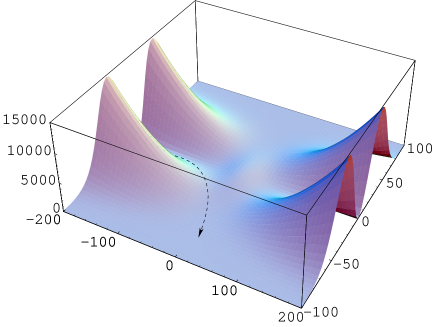
Figure 1: The figure of effective potential (8): $-200<\varphi<200$ and $-100<\sigma<100$. We take $\alpha=\beta=\lambda=10^{-3}$, $\Lambda=10^{3}$ and $\varphi_{*}=\sigma_{*}=1$. In this case, $\varphi_{c}\simeq\pm 24$. The dashing line is one of the motive trajectory of $(\varphi,\sigma)$.

With the increasing of $|\sigma|$ value, the effective potential gradually decreases. Since $\sigma$ is the normal scalar field, its coupling to usual matter is well-defined. In our case, the $\sigma$ field does not oscillate , thus the standard theory of reheating based on the decay of the oscillating field [23, 31] does not apply. The gravitational particle production [32] may be a reheating approach but is not efficient enough. Furthermore, the instant preheating mechanism [24, 25] may be better selection and be more efficient in such non-oscillatory models.

In this scenario, initially the $(\varphi,\sigma)$ is in the bottom of the effective potential, then slow climbs along its valley. During this period, the fluctuations are stretched to outside of horizon and form primordial perturbations on the formation of cosmological structure. A generic potential of simple phantom field relative to this phase can be characterized by two independent mass scales and be written as

$$V(\varphi)=\Lambda f({\varphi\over\varphi_{*}})$$ (11)

where the height $\Lambda$ corresponds the vacuum energy density during phantom inflation and is fixed by normalization, and The width $\varphi_{*}$ corresponds the change of the field value and is a free parameter of models. We will discuss the metric perturbations of various phantom inflation model from such general potential of phantom in the following.

Primordial Perturbations - In longitudinal gauge and in absence of anisotropic stresses, the scalar metric perturbation can be written as

$$ds^{2}=a^{2}(\eta)(-(1+2\Phi)d\eta^{2}+(1-2\Phi)\delta_{ij}dx^{i}dx^{j})$$ (12)

where $\eta$ is conformal time $d\eta={dt\over a}$ and $\Phi$ is the Bardeen potential. Defining the variable [33, 34]

$$v={a\varphi^{\prime}\over{\cal H}}\zeta\equiv z\zeta$$ (13)

where

$$\zeta={1\over\epsilon}({\cal H}\Phi^{\prime}+\Phi)+\Phi$$ (14)

is the curvature perturbation on uniform comoving hypersurfaces, ${\cal H}={a^{\prime}\over a}$ and the prime denotes differentiation with respect to the conformal time $\eta$. In the momentum space, the equation of motion of $v_{k}$ is

$$v_{k}^{\prime\prime}+\left(k^{2}-{z^{\prime\prime}\over z}\right)v_{k}=0.$$ (15)

where

$${z^{\prime\prime}\over z}={1\over\eta^{2}}\left(\nu^{2}-{1\over 4}\right)$$ (16)

and $\nu\simeq{3\over 2}+2\epsilon_{\rm pha}-\delta_{\rm pha}$ to lowest order of $\epsilon_{\rm pha}$ and $\delta_{\rm pha}$. Thus following the same steps as normal scalar field inflation, we obtain

$${\cal P}_{s}={1\over|\epsilon_{\rm pha}|m_{p}^{2}}({h\over 2\pi})^{2}_{k=ah}$$ (17)

and its spectrum index is $n_{s}\simeq 1-4\epsilon_{\rm pha}+2\delta_{\rm pha}$ Similarly for tensor metric perturbation, we obtain

$${\cal P}_{t}={1\over m_{p}^{2}}({h\over 2\pi})^{2}_{k=ah}$$ (18)

and its spectrum index is $n_{t}\simeq-2\epsilon_{\rm pha}$

The tensor/scalar ratio can be expressed as a ratio their contributions to the CMB quadrupole i.e. $r\equiv{C_{2}^{t}\over C_{2}^{s}}$. The relation between $r$ and ratio of amplitudes in the primordial power spectrum ${{\cal P}_{t}\over{\cal P}_{s}}$ depends on the background cosmology. For the currently favored values of $\Omega_{m}\simeq 0.3$ and $\Omega_{\Lambda}\simeq 0.7$, this relation is [35]

$$r\simeq 10|\epsilon_{\rm pha}|$$ (19)

to lowest order. To obtain more insights for the perturbations spectrum of phantom inflation , it may be useful to divide them into three interesting classes compared with normal scalar field inflation, i.e. large field (chaotic inflation [37]), small field (new inflation [2], natural inflation [38]) and hybrid inflation model [27], see Fig. 2. For the case that the maxima of phantom potential are not in $\varphi=0$, like large field and hybrid model, we can carry out a transform $\varphi\rightarrow\varphi-\varphi_{\rm max}$ for $V(\varphi,\sigma)$, which make the hybrid exit mechanism mentioned above still valid.

Figure 2: The sketch of large field, small field, hybrid model of phantom inflation, which may be regarded as the cross-section of the potential of Fig. 1 in $\sigma=0$. For various models, the phantom field $\varphi$ will climb up along its potential i.e. arrowhead direction, when arriving $\varphi_{c}$, the additional normal scalar field $\sigma$ becomes unstable and will roll down along its potential, thus phantom inflation ends.

Large field models - characterized by $\epsilon_{\rm pha}<\delta_{\rm pha}<-\epsilon_{\rm pha}$, in which the phantom field is driven up to larger value. The generic large field potentials are polynomial-like potentials $\Lambda({\varphi\over\varphi_{*}})^{n}$. From (5), we see that when $\varphi\geq m_{p}$, the slow-climb conditions are satisfied. Combining (5) and (19), we have

$$r={5n\over n+2}(n_{s}-1)$$ (20)

which is a blue spectrum and reverse with normal large field inflation models, and when $n\rightarrow\infty$,

$$r=5(n_{s}-1)$$ (21)

which corresponds exponential potentials $\Lambda e^{\varphi\over\varphi_{*}}$. This has been studied in Ref. [20].

Small field models - characterized by $\delta_{\rm pha}>-\epsilon_{\rm pha}$, in which the phantom field is driven up to smaller value. The generic small field potentials are $\Lambda(1-({\varphi\over\varphi_{*}})^{n})$, which may be regarded as a lowest order Taylor expansion of an arbitrary potential about the origin. From (5), we see that when $\varphi\ll\varphi_{*}$, the slow-climb conditions are satisfied. Since $\epsilon_{\rm pha}\sim({\varphi\over\varphi_{*}})^{n}\delta_{\rm pha}$, thus $|\epsilon_{\rm pha}|\ll\delta_{\rm pha}$, the spectrum index is approximately

$$n_{s}-1\simeq 2\delta_{\rm pha}$$ (22)

and tensor perturbation amplitude is suppressed strongly

$$r\simeq 5(n_{s}-1){n\over 2(n-1)}({\varphi\over\varphi_{*}})^{n}$$ (23)

Hybrid models - characterized by $\delta_{\rm pha}<\epsilon_{\rm pha}<0$, in which the phantom field is driven from the bottom with a positive vacuum energy. The generic potentials are $\Lambda(1+({\varphi\over\varphi_{*}})^{n})$. For $\varphi\gg\varphi_{*}$ the models are the same as large field models, and for $\varphi\ll\varphi_{*}$ we have

$$\epsilon_{\rm pha}\simeq-{n^{2}\over 16\pi G\varphi_{*}^{2}}({\varphi\over\varphi_{*}})^{2n-2}$$ (24)

$$\delta_{\rm pha}\simeq{2(n-1)\over n}({\varphi_{*}\over\varphi})^{n}\,\,\epsilon_{\rm pha}$$ (25)

Thus the red spectrum can be obtained only when $|\delta_{\rm pha}|>2|\epsilon_{\rm pha}|$, i.e. ${2(n-1)\over n}({\varphi_{*}\over\varphi})^{n}>2$, and the blue spectrum only when ${2(n-1)\over n}({\varphi_{*}\over\varphi})^{n}<2$.

In addition, there are Linear models, $V(\varphi)\sim\varphi$, which is the boundary between large field and small field models and characterized by $\delta_{\rm pha}=-\epsilon_{\rm pha}$, in which the relation

$$r={5\over 3}(n_{s}-1)$$ (26)

is satisfied.

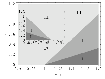
Figure 3: The $r-n_{s}$ figure for phantom inflation models. Inset: The $r-n_{s}$ figure for normal scalar field inflation models [35]. The different shadow Region I II III correspond the different observational parameter space occupied by the small field, large field and hybrid models respectively.

The $r-n_{s}$ plane figure is a powerful tool showing different predictions from various inflation models [36, 35], which is plotted in Fig. 3 for phantom inflation, in which various interesting classes categorized by the slow-climb parameters completely cover the entire $r-n_{s}$ plane. For phantom inflation models, we see that both large field and small field models locate in blue spectrum ($n_{s}>1$) regions, while hybrid models are mainly collected in red spectrum ($n_{s}<1$) regions, which is just reverse with that of normal scalar field inflation models, which is also saw from inset of Fig. 3 [35]. In fact the definition of slow-climb parameters $\epsilon_{\rm pha}$ and $\delta_{\rm pha}$ in phantom inflation is the same as those ($\epsilon_{\rm sca}$ and $\delta_{\rm sca}$) of normal scalar field inflation, but when rewriting these parameters in term of potential of field,

$$\epsilon_{\rm pha}\simeq-{1\over 16\pi G}({V^{\prime}(\varphi)\over V(\varphi)})^{2}$$ (27)

$$\delta_{\rm pha}\simeq{1\over 8\pi G}\left({1\over 2}({V^{\prime}(\varphi)\over V(\varphi)})^{2}-{V^{\prime\prime}(\varphi)\over V(\varphi)}\right)$$ (28)

the interesting results $\epsilon_{\rm pha}=-\epsilon_{\rm sca}$ and $\delta_{\rm pha}=-\delta_{\rm sca}$ are found, which is the main reason that the reverse results of $r-n_{s}$ figure are lead to and reflects the generic features of phantom inflation.

In summary, we study the various models, exit mechanism and primordial perturbation spectrum of phantom inflation and discuss their different features from those of normal scalar field inflation. We proposed an exit mechanism, in which the phantom field climbs up along its potential from the bottom of valley, and when arriving some value, the energy of its potential decays into radiation by the instability of an additional normal scalar field. For the perturbation spectrum, phantom inflation models completely cover the entire $r-n_{s}$ plane, in which the interesting constraints are being placed by the observations [39, 40] and may be tightened in coming years, but with reverse results from those of normal scalar field inflation. In some sense of inflation, phantom inflation may be regarded as a new class different from normal scalar field inflation and worth studying further.

Acknowledgments We thank Bo Feng, Zong-Kuan Guo, Mingzhe Li, Xinmin Zhang for helpful discussions. This work is supported in part by K.C.Wang Postdoc Foundation and also in part by the National Basic Research Program of China under Grant No. 2003CB716300.

References

- [1] A.H. Guth, Phys. Rev. D23 (1981) 347;
- [2] A.D. Linde, Phys. Lett. B108 (1982) 389; A.A. Albrecht and P.J. Steinhardt, Phys. Rev. Lett. 48 (1982) 1220.
- [3] A.D. Linde, hep-th/0402051.
- [4] R.R. Caldwell, Phys. Lett. B545 23 (2002).
- [5] U. Alam, V. Sahni, T.D. Saini A.A. Starobinsky, astro-ph/0311364.
- [6] T.R. Choudhury and T. Padmanabhan, astro-ph/0311622.
- [7] J.S. Alcaniz, astro-ph/0312424.
- [8] S.M. Carroll, M. Hoffman and M. Trodden, Phys. Rev. D68 023509 (2003).
- [9] J.M. Cline, S. Jeon and G.D. Moore, hep-ph/0311312.
- [10] H.P. Nilles, Phys. Rept. 110 1 (1984).
- [11] B. Boisscau, G. Esposito-Farese, d. Polarski and A.A. Starobinsky, Phys. Rev. lett. 85 2236(2000).
- [12] M.D. Pollock, Phys. Lett. B215, 635 (1988).
- [13] V. Sahni and Y. Shtanov, astro-ph/0202346.
- [14] C. Armendariz-Picon, T. Damour and V. Mukhanov, hep-th/9904075; T. Chiba, T. Okabe and M. Yamaguchi, Phys. Rev. D62 023511 (2000); P. F. Gonzalez-Diaz, astro-ph/0312579.
- [15] L.P. Chimento and R. Lazkoz, Phys. Rev. Lett. 91 211301 (2003).
- [16] H. Stefancic, astro-ph/0312484.
- [17] P. Frampton, astro-ph/0209037; B. McInnes, astro-ph/0210321.
- [18] V. Sahni and A. Starobinsky, astro-ph/9904398; L. Parker and A. Raval, Phys. Rev. D60 063512 (1999); A.E. Schulz, M. White, Phys. Rev. D64 043514 (2001); V.K. Onemli,and R.P. Woodard, Class. Quant. Grav. 19 4607 (2002); D.R. Torres, Phys. Rev. D66 043522 (2002); S. Hannestad and E. Mortsell, Phys. Rev. D66 063508 (2002); A. Melchiorri, L. Mersini, C.J. Odman and M. Trodden, Phys. Rev. D68 043509 (2003).
- [19] G.W. Gibbons, hep-th/0302199; R.R. Caldwell, M. Kamionkowski and N.N. Weinberg, astro-ph/0302506; S. Nojiri and S.D. Odintsov, hep-th/0303117; hep-th/0304131; hep-th/0306212; P. Singh, M. Sami and N. Dadhich, hep-th/0305110; A. Feinstein and S. Jhingan, hep-th/0304069; A. Yurov, astro-ph/0305019; P.F. Gonzalez-Diaz, astro-ph/0305559; M.P. Dabrowski, T. Stachowiak and M. Szydlowski, hep-th/0307128; H. Stefancic, astro-ph/0310904 X.H. Meng and P. Wang, hep-ph/0311070, V.B. Johri,astro-ph/0311293; J.M. Aguirregabiria, L.P. Chimento and R. Lazkoz astro-ph/0403157; L.P. Chimento, R. Lazkoz, gr-qc/0405020.
- [20] Y.S. Piao and E Zhou, Phys. Rev. D68, 083515 (2003).
- [21] M. Sami and A. Toporensky gr-qc/0312009.
- [22] P.F. Gonzalez-Diaz, Phys.Rev. D68, 084016 (2003).
- [23] L. Kofman, A.D. Linde and A.A. Starobinski, Phys. Rev. Lett. 73 3195 (1994); Phys. Rev. D56 3258 (1997).
- [24] G.N. Felder, L. Kofman and A.D. Linde, Phys. Rev. D59 123523 (1999).
- [25] G.N. Felder, L. Kofman and A.D. Linde, Phys. Rev. D60 103505 (1999).
- [26] B. McInnes, JHEP 0208 029 (2002).
- [27] A.D. Linde, Phys. Lett. B259 38 (1991); Phys. Rev. D49 748 (1994).
- [28] E.J. Copeland, A.R. Liddle, D.H. Lyth, E.D. Stewart and D. Wands, Phys. Rev. D49 6410 (1994).
- [29] J. Garcia-Bellido, A.D. Linde, D. Wands, Phys.Rev. D54 6040 (1996).
- [30] in preparation.
- [31] J. Garcia-Bellido and A.D. Linde, Phys.Rev. D57 6075 (1998).
- [32] L.H. Ford, Phys. Rev. D35 2955 (1987).
- [33] V.F. Mukhanov, JETP lett. 41, 493 (1985); Sov. Phys. JETP. 68, 1297 (1988).
- [34] V.F. Mukhanov, H.A. Feldman and R.H. Brandenberger, Phys. Rept. 215, 203 (1992).
- [35] W.K. Kinney, E.W. Kolb, A. Melchiorri and A. Riotto, hep-ph/0305130.
- [36] S. Dodelson, W.H. Kinney and E.W. Kolb, Phys. Rev. D56 3207 (1997); W.H. Kinney, Phys. Rev. D58 123506 (1998).
- [37] A.D. Linde, Phys. Lett. B129 177 (1983).
- [38] K. Freese, J. Frieman and A. Olinto, Phys. Rev. Lett. 65 3233 (1990).
- [39] C. L. Bennett et al., astro-ph/0302207; E. Komatsuet al., astro-ph/0302223.
- [40] M. Tegmark et al., astro-ph/0310723.