Water masers in dusty environments

We study in details a pumping mechanism for the $\lambda=1.35$ cm maser transition $6_{16}\rightarrow 5_{23}$ in ortho-H₂O based on the difference between gas and dust temperatures. The upper maser level is populated radiatively through $4_{14}\rightarrow 5_{05}$ and $5_{05}\rightarrow 6_{16}$ transitions. The heat sink is realized by absorbing the 45 $\mu{\rm m}$ photons, corresponding to the $5_{23}\rightarrow 4_{14}$ transition, by cold dust. We compute the inversion of maser level populations in the optically thick medium as a function of the hydrogen concentration, the gas-to-dust mass ratio, and the difference between the gas and the dust temperatures. The main results of numerical simulations are interpreted in terms of a simplified four-level model. We show that the maser strength depends mostly on the product of hydrogen concentration and the dust-to-water mass ratio but not on the size distribution of the dust particles or their type. We also suggest approximate formulae that describe accurately the inversion and can be used for fast calculations of the maser luminosity. Depending on the gas temperature, the maximum maser luminosity is reached when the water concentration $N_{\rm H_{2}O}\approx 10^{6}\div 10^{7}{\rm cm}^{-3}$ times the dust-to-hydrogen mass ratio, and the inversion completely disappears at density just an order of magnitude larger. For the dust temperature of 130 K, the $6_{16}\rightarrow 5_{23}$ transition becomes inverted already at the temperature difference of $\Delta T\sim 1$ K, while other possible masing transitions require a larger $\Delta T\gtrsim 30$ K. We identify the region of the parameter space where other ortho- and para-water masing transitions can appear.

1 Introduction

Sources of strong water maser emission at wavelength $\lambda=1.35$ cm have been found in many astrophysical objects such as active galactic nuclei, carbon rich stars, protostellar regions and comets. Maser emission is a powerful tool for investigating the physical conditions in the emitting regions because of its high brightness as well as a high sensitivity to the physical parameters of the medium in which the maser amplification takes place.

There are several mechanisms for the ortho-H₂O $6_{16}\rightarrow 5_{23}$ ($\lambda=1.35$ cm) maser pumping. de Jong (1973) proposed a comprehensive model where the breakdown of thermal equilibrium occurs in the surface layers of the dense gas cloud. Upon approach to the surface, the $5_{23}\rightarrow 4_{14}$ transition (45 $\mu{\rm m}$) (which is among the most important for the maser action, see Fig.  1) becomes transparent first and level $5_{23}$ becomes underpopulated. The de Jong model was widely used to describe the water masers from late-type stars and star-forming regions (Cooke & Elitzur 1985; Elitzur, Hollenbach, & McKee 1989; Neufeld & Melnick 1991), and the molecular accretion disks in active galactic nuclei (Neufeld, Maloney, & Conger 1994; Babkovskaya & Varshalovich 2000).

The de Jong mechanism is, however, not able to explain the most powerful masers in star-forming regions. A different physics has to be involved. In shocks, the departures from the equilibrium could be produced by collisions with hotter “superthermal” hydrogen gas (Varshalovich et al. 1983). Strelnitskij (1980, 1984) proposed that collisions with two species (e.g. charged and neutral particles) of different temperatures and with comparable collision rate can produce the necessary inversion at high hydrogen densities needed to explain the high observed maser luminosities. Kylafis & Norman (1987) pointed out that the magnetohydrodynamic shocks produce naturally conditions where the electron temperature $T_{\rm e}$ is larger than the hydrogen temperature $T_{\rm H}$. In such a case, the lower maser level becomes underpopulated, because the relative importance of collisions with neutrals is larger for the transitions to/from this level. The inversion in this model appeared only in a narrow range of the ionization fraction $10^{-5}-10^{-4}$ and for $T_{\rm H}<60$ K. At high ionization, electrons start to dominate the collisions and the levels are thermalized at $T_{\rm e}$, while at lower ionization, neutrals are dominating and the thermalization happens at $T_{\rm H}$. Using better estimates for the collision rates, Elitzur & Fuqua (1989) and Anderson & Watson (1990) ruled out this model unless the neutral particles are hotter than the charged ones, conditions that are difficult to imagine in any astrophysical environment.

All astrophysical objects that show water maser emission are also expected to have non-negligible quantities of dust. If the dust and the gas have different temperatures, the departures from the equilibrium are possible (Goldreich & Kwan 1974; Kegel 1975; Strelnitskij 1977; Bolgova et al. 1977). Goldreich & Kwan (1974) suggested that the radiation from the hot dust excites the water molecules to the vibrational state, and the heat sink is provided by collisions with cooler (than dust) hydrogen molecules. The possibility of the inversion in such a situation was questioned by Deguchi (1981) who pointed out that because the collisional de-excitation rate between vibrational states is much smaller than the pure-rotational collisional rate, the rotational collisional thermalization may quench the maser when vibrational collisional de-excitation becomes dominant (see also Strelnitskij 1988).

Alternatively, the cold dust can produce the necessary inversion (Strelnitskij 1977; Bolgova et al. 1977). In the optically thick environment, the excitation temperature takes the values between the dust and the gas temperatures depending on the relative role of dust and collisions in the destruction of the line photons. Deguchi (1981) considered the following cycle of the maser levels pumping $4_{14}\rightarrow 5_{05}\rightarrow 6_{16}\rightarrow 5_{23}\rightarrow 4_{14}$ (see Fig. 1). He showed that the downward transition $5_{23}\rightarrow 4_{14}$ at 45 $\mu{\rm m}$ is much more affected by the dust absorption than the upward transitions at $\lambda\sim 80-100\ \mu{\rm m}$, because there is a strong peak near 45 $\mu{\rm m}$ in the absorption coefficient of the cosmic-type ices (e.g. Moore & Hudson 1994). The upper level excitation temperature is then close to the gas temperature, while the lower level becomes populated at the dust temperature. Similar inversion occurs for other types of dust too.

One should note that in this model an arbitrary thick layer can participate in the maser action provided the gas and dust temperatures sufficiently differ. Chandra et al. (1984a) computed the maser efficiency when both the surface escape and the cold dust absorption mechanisms operate together. Recently Collison & Watson (1995) and Wallin & Watson (1997) applied this model to the masing disk in the active galaxy NGC 4258 concluding that the cold dust model is much more efficient (see also Neufeld 2000). Thus the cold dust–hot gas model seems to be the most promising to explain powerful water masers in many astrophysical objects. The temperature difference between the gas and the dust can appear as a result of shock heating or illumination by the UV- or X-ray photons, and/or because of the presence of the dust particles of different types and sizes which assure different temperatures.

The purpose of the present study is to determine the maser strength for a broad range of the physical parameters: the hydrogen concentration, the water-to-dust mass ratio, the gas and the dust temperatures as well as the dust type. Previous studies (Deguchi 1981; Chandra et al. 1984a) used the rectangular line profile instead of the Doppler one as well as the collisional coefficients with hydrogen of Green (1980), which later have been much improved (Green, Maluendes, & McLean 1993). Only a handful set of parameters was explored in the more recent investigation of Collison & Watson (1995) and Wallin & Watson (1997) who considered the case of saturated maser.

In its full statement this problem needs the simultaneous solution of the statistical balance equations together with the radiative transfer equations for all spectral lines. However, because the cold dust – hot gas model can operate inside a molecular cloud where almost all transitions (except masing) are optically thick, the radiative transfer can be handled in a very simple manner using the escape probability formalism, where now the role of the escape of spectral line photons is played by the dust absorption.

The paper is constructed as follows. We give the formulation of the problem and describe the numerical method in Sect. 2. We develop a simple four-level model that contains most of the physics involved in Sect. 3. The numerical results for different dust types and size distributions are presented in Sect. 4, where we also propose simple analytical formulae for the inversion which describe the results of simulations. Finally, in Sect. 5 we present our conclusions.

Figure 1: A portion of the diagram of the ortho-H₂O showing rotational levels involved in the pumping of $6_{16}\rightarrow 5_{23}$ maser.

2 Method

2.1 Radiative transfer

We consider a slab consisting of a mixture of molecular hydrogen, water molecules and dust particles. The radiative transfer equation for the specific intensity $I_{x}$ describing the transfer of the line radiation in the presence of the continuum absorption and emission is (Hummer 1968; Mihalas 1978)

$$\mu\frac{{\rm d}I_{x}}{{\rm d}z}=-(\alpha_{\rm L}\phi_{x}+\alpha_{\rm d})I_{x}+\alpha_{\rm L}\phi_{x}S_{{ul}}+\alpha_{\rm d}B_{{ul}}(T_{\rm d}),$$ (1)

where $z$ is the geometrical depth, $\mu$ is the cosine of the angle between the direction of propagation and the outward normal,

$$S_{{ul}}=\left(\frac{n_{{l}}}{n_{{u}}}\frac{g_{{u}}}{g_{{l}}}-1\right)^{-1},\;\;{u}>{l},$$ (2)

is the source function for the line transition between the energy levels ${u}$ and ${l}$, and $B_{{ul}}(T_{\rm d})$ is the Planck function at the transition frequency $\nu_{{ul}}$ characterized by the dust temperature. All the intensities and the source functions are given in units $2h\nu_{{ul}}^{3}/c^{2}$. The dust absorption coefficient $\alpha_{\rm d}=\kappa_{\rm d}\rho_{\rm d}$ depends on the frequency-dependent (constant within the line) opacity $\kappa_{\rm d}\ [{\rm cm}^{2}{\rm g}^{-1}]$ and the dust density $\rho_{\rm d}=f_{\rm d}2m_{\rm p}N_{\rm H_{2}}\ [{\rm g}\ {\rm cm}^{-3}]$, where $m_{\rm p}$ is the proton mass, $N_{\rm H_{2}}$ is the concentration of molecular hydrogen, and $f_{\rm d}$ is the dust-to-hydrogen mass ratio.

The line averaged absorption coefficient $\alpha_{\rm L}$ (including induced emission) depends on the corresponding level populations:

$$\alpha_{\rm L}=g_{{u}}A_{{ul}}\Delta n_{{ul}}\frac{\lambda_{{ul}}^{3}}{8\pi c(\Delta\nu_{\rm D}/\nu_{{ul}})}N_{\rm H_{2}O},$$ (3)

where $\Delta n_{{ul}}=\frac{n_{{l}}}{g_{{l}}}-\frac{n_{{u}}}{g_{{u}}}$, $n_{{u}}$ is the fractional level population ($\sum_{u}n_{{u}}=1$), $N_{\rm H_{2}O}$ is the water concentration, $g_{{u}}$ is the statistical weight for a given level, $A_{{ul}}$ is the Einstein coefficient, and $\lambda_{{ul}}=c/\nu_{{ul}}$ is the transition wavelength. We further assume complete frequency redistribution within the line, i.e. both the absorption and emission line profile are described by the same function $\phi_{x}$ normalized as $\int\phi_{x}{\rm d}x=1$, where $x=(\nu-\nu_{{ul}})/\Delta\nu_{\rm D}$ is the frequency within the spectral line in thermal Doppler units $\Delta\nu_{\rm D}=\nu_{{ul}}(2kT/mc^{2})^{1/2}$. For the Doppler profile assumed here, $\phi_{x}=\pi^{-1/2}\exp(-x^{2})$.

Let us note the averaged over line profile optical thickness of the slab in ${ul}$–line as $2\tau_{0}=\int\alpha_{\rm L}{\rm d}z$. A formal solution of the radiative transfer equation (1) for a homogeneous (i.e. $T=const,T_{\rm d}=const$) slab gives the mean intensity of the radiation averaged over the line profile at the optical depth $\tau$ (Hummer 1968; Mihalas 1978):

$$\overline{J_{{ul}}}(\tau) = \int\phi_{x}J_{x}(\tau){\rm d}x=(1-\delta)\int_{0}^{2\tau_{0}}S_{{ul}}(t)K_{1}(t-\tau){\rm d}t$$ (4)

$$+ \delta B_{{ul}}(T_{\rm d})\int_{0}^{2\tau_{0}}L_{1}(t-\tau){\rm d}t,$$

where the kernels

$$K_{1}(s) = \frac{1}{2(1-\delta)}\int E_{1}\left([\phi_{x}+\beta]|s|\right)\phi_{x}^{2}{\rm d}x,$$ (5)

$$L_{1}(s) = \frac{\beta}{2\delta}\int E_{1}\left([\phi_{x}+\beta]|s|\right)\phi_{x}{\rm d}x$$ (6)

are normalized as $\int_{-\infty}^{\infty}K_{1}(t){\rm d}t=\int_{-\infty}^{\infty}L_{1}(t){\rm d}t=1$. Here $E_{n}(\tau)=\int_{0}^{1}\mu^{n-2}\exp(-\tau/\mu){\rm d}\mu$ is the exponential integral function,

$$\beta=\alpha_{\rm d}/\alpha_{\rm L},$$ (7)

and

$$\delta=\beta\int\frac{\phi_{x}}{\phi_{x}+\beta}{\rm d}x$$ (8)

(index $ul$ is omitted in $\beta$ and $\delta$ as well as in the formulae below) is the probability per single interaction act that the line photon will be absorbed by dust (obviously, $1-\delta$ is the probability for a photon to excite a molecule).

If the source function does not vary much, we can take it out from the integral (the so called on-the-spot or the first order escape probability approximation) and get:

$$\overline{J}(\tau) \simeq (1-\delta)\left[1-\frac{1}{2}K_{2}(\tau)-\frac{1}{2}K_{2}(2\tau_{0}-\tau)\right]S(\tau)$$

$$+ \delta\left[1-\frac{1}{2}L_{2}(\tau)-\frac{1}{2}L_{2}(2\tau_{0}-\tau)\right]B(T_{\rm d})$$

$$= (1-p)S+p^{\rm c}B(T_{\rm d}),$$

where

$$K_{2}(\tau) = 2\int_{\tau}^{\infty}K_{1}(t){\rm d}t$$ (10)

$$= \frac{1}{1-\delta}\int\frac{\phi_{x}^{2}}{\phi_{x}+\beta}E_{2}\left([\beta+\phi_{x}]\tau\right)\;{\rm d}x,$$

$$L_{2}(\tau) = 2\int_{\tau}^{\infty}L_{1}(t){\rm d}t$$ (11)

$$= \frac{\beta}{\delta}\int\frac{\phi_{x}}{\phi_{x}+\beta}E_{2}\left([\beta+\phi_{x}]\tau\right)\;{\rm d}x.$$

For every column density of the slab we can take the intensity in the middle plane $\overline{J}(\tau_{0})$ as the representative one. We perform all our calculations using equation (2.1) with $\tau=\tau_{0}=\alpha_{\rm L}H$ (where $H$ is the slab half-thickness), i.e taking

$$p=\delta+(1-\delta)K_{2}(\tau),\quad p^{\rm c}=\delta[1-L_{2}(\tau)].$$ (12)

If, however, the line is optically thick, the escape is negligible and the mean intensity is simply

$$\overline{J}\simeq(1-\delta)S+\delta B(T_{\rm d}).$$ (13)

This expression can be obtained directly from equation (1) assuming isotropic intensity of radiation (i.e. assuming ${\rm d}I_{x}/{\rm d}z=0$ and $I_{x}=J_{x}$), solving for $J_{x}$, and integrating it over the frequency with a weight $\phi_{x}$. If most of the considered lines are optically thick, the populations do not depend on the optical depth of the considered point but are determined by the local conditions (such as hydrogen density, gas-to-dust density ratio, and dust and gas temperatures) only.

Following Hollenbach & McKee (1979), we approximate $\delta(\beta)$ as

$$\delta\simeq\frac{2\beta}{1+2\beta}\left[\ln{\left({\rm e}+\frac{1}{\sqrt{\pi}\beta}\right)}\right]^{1/2}$$ (14)

and slightly modify the expression for $K_{2}(\tau)$:

$$K_{2}(\tau)\simeq\frac{\exp(-\tau_{\rm d})}{1+(1-\delta)\sqrt{\tau_{\rm d}}}\ \frac{1}{1+\tau_{\rm c}[2\pi\ln(2.13+\tau_{\rm c}^{2})]^{1/2}},$$ (15)

where $\tau_{\rm c}=\tau/\sqrt{\pi}$ is the optical depth in the line center and $\tau_{\rm d}=\beta\tau$ is the optical depth for the dust absorption. The continuum escape coefficient $p^{\rm c}=\delta[1-L_{2}(\tau)]$ is approximated as

$$p^{\rm c} \simeq X\left(\delta-\frac{\exp(-\tau_{\rm d})}{1+\tau_{\rm c}[\pi\ln(1.25+\tau_{\rm c})]^{1/2}}\right.$$ (16)

$$\times \left.\frac{\delta+\tau_{\rm d}[1-\ln(1+1/\tau_{*})]}{1+\tau_{\rm d}}\right),$$

$$X = 1-0.095\frac{y}{1+y^{2}}\ln(1+0.028/\beta),$$

where $y=(0.477\tau_{\rm c})^{0.277}$, $\tau_{*}=\max(\tau_{\rm d},\tau_{\rm c})$. These expressions for $K_{2}$ and $p^{\rm c}$ are accurate within $10\%$ for any $\beta$ and $\tau$.

The masing lines need a different treatment. We neglect the dust influence in such transitions, i.e. assume $\beta=\delta=p^{\rm c}=0$. Using expression (10), one can show that at large maser optical depth $|\tau|\gg 1$

$$K_{2}(\tau)\sim\frac{\exp(|\tau_{\rm c}|)}{|\tau_{\rm c}|\sqrt{\pi\ln|\tau_{\rm c}|}}.$$ (17)

Then the line escape coefficient for $\tau<0$ can be represented as

$$p(\tau)=\frac{\exp(|\tau_{\rm c}|)+1.18|\tau_{\rm c}|}{1+|\tau_{\rm c}|\ [\pi\ln(1+|\tau_{\rm c}|)]^{1/2}}.$$ (18)

This expression reproduces the exponential asymptotic behavior at large $|\tau_{\rm c}|$ (17) as well as matches the asymptotic of $K_{2}$ at small $\tau_{\rm c}$ (see eq. 15).

We consider different types of dust. The amorphous ice absorption coefficient is computed from the optical constants of Leger et al. (1983). The crystalline ice absorption coefficient are based on the data from Bertie et al. (1969) and Warren (1984). The silicate and graphite data are from Laor & Draine (1993).

2.2 Statistical balance equations

The populations of $M$ levels can be determined from the population balance equations which, in the stationary case, take the form:

$$\sum_{{l}\neq{u}}n_{{l}}\,W_{{lu}} = n_{{u}}\sum_{{l}\neq{u}}W_{{ul}},\quad{u}=1,2\ldots,M-1,$$ (19)

$$\sum_{{u}=1}^{M}n_{{u}} = 1,$$

where $W_{{ul}}=C_{{ul}}+R_{{ul}}$ is the total rate of the ${u}\rightarrow{l}$ transition,

$$C_{{lu}}^{\uparrow}=\frac{g_{{u}}}{g_{{l}}}C_{{ul}}^{\downarrow}\exp\left(-\frac{h\nu_{{ul}}}{kT}\right),\qquad C_{{ul}}^{\downarrow}=N_{\rm H_{2}}k_{{ul}}(T)$$ (20)

being the rates of the collisional excitation and deexcitation of water molecules by molecular hydrogen which kinetic temperature equals that of the water. The rates of the radiative excitation and deexcitation are given by

$$R_{{lu}}^{\uparrow}=A_{{ul}}\frac{g_{{u}}}{g_{{l}}}\overline{J_{{ul}}},\qquad R_{{ul}}^{\downarrow}=A_{{ul}}\left(1+\overline{J_{{ul}}}\right).$$ (21)

The Einstein A-coefficients are taken from Chandra et al. (1984b). Collisional deexcitation rates are from Green, Maluendes, & McLean (1993), while the excitation rates are computed using the detailed balance condition. We take into account the first 45 rotational levels of ortho- and para-H₂O molecules and all possible radiative and collisional transitions between them.

Substituting the radiation intensity from (2.1) into (21) and the statistical balance equations (19), we obtain:

$$\sum_{{l}>{u}}A_{{lu}}\left(p_{{lu}}n_{{l}}+p^{\rm c}_{{lu}}B^{\rm d}_{{lu}}g_{{l}}\Delta n_{{ul}}\right)$$

$$- \sum_{{l}<{u}}A_{{ul}}\left(p_{{ul}}n_{{u}}+p^{\rm c}_{{ul}}B^{\rm d}_{{ul}}g_{{u}}\Delta n_{{lu}}\right)$$

$$= \sum_{{l}\neq{u}}\left(C_{{ul}}n_{{u}}-C_{{lu}}n_{{l}}\right),\quad u=1,2,\dots,M-1,$$

with the same normalization as before $\sum_{{u}}n_{{u}}=1$.

The populations can be found from the solution of the system of non-linear algebraic equations (12), (18), and (2.2). We use the Newton-Raphson method with line searches and backtracking (Press et al. 1992). We normally start from high hydrogen density where the solution is close to the Boltzmann at the gas temperature and use the obtained solution as a zeroth approximation for the next point. We continue iterations until the maximum error in the system becomes smaller than $10^{-11}$ and the maximal change in populations is smaller than $10^{-9}$. It takes 5 to 15 iterations for most sets of parameters and each computation takes on average about 15 ms CPU time on a Pentium IV 2 GHz Linux PC.

2.3 Maser intensity

If the maser amplification takes in the homogeneous medium and there is no velocity gradients, the maser intensity can be estimated as

$$I_{x}(\tau_{\rm m})\simeq(I_{0}+|S_{\rm m}|)\exp(\tau_{\rm m}\phi_{x}),$$ (23)

where $I_{0}$ is the background continuum intensity, $S_{\rm m}$ is the source function for the ${u}\rightarrow{l}$ masing transition, and the optical depth in the maser line $\tau_{\rm m}$ is

$$\tau_{\rm m}=\alpha_{\rm m}L_{\rm coh}=\frac{\lambda_{{ul}}^{3}g_{{u}}A_{{ul}}}{8\pi c(\Delta\nu_{\rm D}/\nu_{{ul}})}\Delta n_{\rm m}N_{\rm H_{2}O}L_{\rm coh},$$ (24)

where $\Delta n_{\rm m}=n_{{u}}/g_{{u}}-n_{{l}}/g_{{l}}$ (positive for the maser) and $L_{\rm coh}$ is the typical coherent length of the maser amplification. If the excitation temperature of the masing transition is larger than the brightness temperature of the background, one can neglect $I_{0}$ (and obviously other way around too). We assumed the first possibility (i.e. $I_{0}=0$). In this paper we quote values of $\tau_{\rm m}$ for $L_{\rm coh}=H$. Obviously, at grazing angles to the slab surface this value can be exceeded many times.

2.4 Parameter range

The water level populations depend on the hydrogen density $N_{\rm H_{2}}$, the dust and water concentrations and temperatures as well as the slab half-thickness $H$. When the photon escape from the surface is negligible because the slab is optically thick either in continuum ($\tau_{\rm d}\gtrsim 1$) or in the line ($\tau\gg 1$), the terms $K_{2}$ and $L_{2}$ can be omitted in the escape probabilities (12) (i.e. $p=p^{\rm c}=\delta$). The solution of the population balance equations then depends on $\delta$, which in turn depends only on the ratio of the absorption coefficients $\beta$, but not on the absorption coefficients individually. Since the dust opacity $\kappa_{\rm d}$ has a rather weak dependence on the size of the dust particles, it is rather natural to use the water-to-dust mass ratio $f_{\rm H_{2}O}/f_{\rm d}$ as a parameter, where $f_{\rm H_{2}O}$ is the water-to-hydrogen mass ratio and $f_{\rm d}$ is the dust-to-hydrogen mass ratio. The water concentraion relates then to these parameters through $N_{\rm H_{2}O}=N_{\rm H_{2}}(f_{\rm H_{2}O}/f_{\rm d})f_{\rm d}/9$ (factor 9 comes from the ratio $m_{\rm H_{2}O}/m_{\rm H_{2}}$). When the escape through the surface is small and masers are unsaturated (i.e. a masing transition does not affect the level populations), the populations do not depend on $f_{\rm d}$ and the scale-height $H$, and the optical depth is then linearly proportional to $f_{\rm d}H$. In such a situation the main parameters are $N_{\rm H_{2}}$, $f_{\rm H_{2}O}/f_{\rm d}$, $T$ and $T_{\rm d}$. If the dust is suffiently cold, its own radiation is then negligible and dependence on $T_{\rm d}$ disappears. We normally consider the dust colder than the gas, $\Delta T\equiv T-T_{\rm d}>0$, because this is required for inversion to occur (in the optically thick case).

One can also point out that for large $f_{\rm H_{2}O}/f_{\rm d}$ when $\beta\sim\delta\ll 1$ in the main infrared pumping lines, the solution of the balance equations (2.2) depends on the product $N_{\rm H_{2}}f_{\rm H_{2}O}/f_{\rm d}$, but not on $N_{\rm H_{2}}$ and $f_{\rm H_{2}O}/f_{\rm d}$ individually, because $C_{{ul}}/p_{{ul}}\propto N_{\rm H_{2}}/\beta\propto N_{\rm H_{2}}f_{\rm H_{2}O}/f_{\rm d}$.

We consider a range of the hydrogen concentrations from $10^{8}$ to $10^{12.5}{\rm cm}^{-3}$. At higher $N_{\rm H_{2}}$, the inversion is absent because of the thermalization by collisions with the hydrogen molecules, while at smaller $N_{\rm H_{2}}$ we can extrapolate the results from $N_{\rm H_{2}}=10^{8}$.

In astrophysical objects it is easier to estimate the dust-to-gas mass ratio $f_{\rm d}$ than other parameters of interest. We fix it at a standard for the interstellar medium value of $f_{\rm d}=0.01$. This then determines the dust optical depth

$$\tau_{\rm d}=0.033\kappa_{\rm d}\frac{N_{\rm H_{2}}}{10^{10}}\frac{f_{\rm d}}{0.01}\frac{H}{10^{14}}.$$ (25)

For the majority of calculations we consider the dust in the form of the amorphous ice grains of the size $a=0.1\ \mu{\rm m}$. Comparison is also made to different sizes and temperatures of dust as well as other types of dust (crystalline ice, silicate, and graphite).

The water-to-dust mass ratio probably varies by orders of magnitude from one object to another. Therefore, we consider a broad range of $f_{\rm H_{2}O}/f_{\rm d}$ from $10^{-8}$ to $10^{0}$. The maximum possible $f_{\rm H_{2}O}$ in the interstellar medium is about $10^{-3}$ which transforms to the maximum $f_{\rm H_{2}O}/f_{\rm d}\sim 0.1$ for $f_{\rm d}=0.01$. However, for a smaller dust content, $f_{\rm H_{2}O}/f_{\rm d}$ can be larger.

Figure 2: Dependence of the $6_{16}$–$5_{23}$ maser absorption coefficient $\alpha_{\rm m}/(10^{-14}{\rm cm}^{-1})$ on the half-thickness of the slab for six sets of parameters $(N_{\rm H_{2}},f_{\rm H_{2}O}/f_{\rm d})$: (1) $10^{9},10^{-2}$; (2) $10^{10},10^{-3}$; (3) $10^{11},10^{-4}$; (4) $10^{9},10^{-4}$; (5) $10^{10},10^{-5}$; (6) $10^{11},10^{-6}$. Other parameters are fixed at $T_{\rm d}=130$ K, $T=250$ K, $f_{\rm d}=0.01$. At a slab thickness less that $10^{13}$ cm, the effect of the boundary becomes significant. For higher $H$, the maser becomes saturated when $\tau_{\rm m}=30$.

Figure 2 shows the absolute value of the absorption coeffient (in units of $10^{-14}{\rm cm}^{-1}$) in the main masing line $6_{16}\rightarrow 5_{23}$ for six representative sets of parameters $(N_{\rm H_{2}},f_{\rm H_{2}O}/f_{\rm d})$. One sees that at $H\lesssim 10^{13}$ cm, the surface escape of photons (the de Jong mechanism) starts to influence the populations. At high $H$, the optical depth $\tau_{\rm m}$ can be sufficiently large to saturate the maser. One can easily estimate the optical depth when it happens. The saturation occurs when the induced transition rate $A\overline{J}$ in the masing line becomes comparable to the rates of transitions from the upper masing level in other strong lines (see eq. 21) which are $R_{{ul}}\sim 1$. Because the Einstein $A$ coefficient in the 1.35 cm $6_{16}\rightarrow 5_{23}$ masing line is about $10^{-9}$ (and about $10^{-5}$ in other masing transitions), the saturation occurs when $\overline{J}\sim 10^{9}$. On the other hand, since

$$\overline{J}\sim p|S|\sim\exp(\tau_{\rm m}/\sqrt{\pi})|S|$$ (26)

(see eq. 18) and $|S|\sim 30$, the maser saturates at the optical depth $\tau_{\rm m}\sim 30$ (which weakly depends on the value of $S$). This limiting optical depth is reached at different $H$ depending on the conditions. Here the maser saturates and the inversion decreases.

The inversion is rather flat around $H\sim 10^{14}$ cm, where it is a function of the local conditions only. Therefore, we use this height for our calculations. We should also note that our results do not depend on the geometry of the system, and can be applied not only to the slab but to any other geometry.

The contours of the constant maser absorption coefficient and the optical depth on a plane $H$ - gas temperature $T$ are shown in Fig. 3. One sees that, independently of the gas temperature, the absorption coefficient is rather flat around $H\sim 10^{14}$ cm. The flat part becomes shorter at higher gas temperature, because the saturation ($\tau_{\rm m}\sim 30$) happens for smaller $H$. One should note here that the parameter set $N_{\rm H_{2}},f_{\rm H_{2}O}/f_{\rm d}$ taken at this graph gives much shorter flat parts than other sets presented in Fig. 2. Our fiducial $H=10^{14}$ cm still seems to be a good choice for studying in details the physics of the unsaturated water maser in a dusty environment. It is also interesting to note that for small $H$ inversion exist even when $T<T_{\rm d}$ because of the action of the de Jong mechanism.

Figure 3: Levels of the constant maser absorption coefficient $\alpha_{\rm m}/(10^{-14}{\rm cm}^{-1})$ (solid curves) and the maser optical depth $\tau_{\rm m}$ (dotted curves) on the plane slab half-thickness – gas temperature for $N_{\rm H_{2}}=10^{9}{\rm cm}^{-3}$ and $f_{\rm H_{2}O}/f_{\rm d}=10^{-2}$. Other parameters are fixed at $T_{\rm d}=130$ K, $f_{\rm d}=0.01$.

3 Analytical four level model

Our main goal is to study in details the inversion mechanism of the $6_{16}\rightarrow 5_{23}$ masing transition. Before we proceed to the results of calculations, it is useful to understand the physical processes responsible for the action of this main maser using a simplified system of molecular levels, which mainly participate in the maser pumping: $4_{14}$ (level 1), $5_{05}$ (level 2), $5_{23}$ (level 3) and $6_{16}$ (level 4) (see Fig. 1 and Deguchi 1981). The upper maser level 4 interacts mostly with the 2nd level which in turn interacts with level 1, while the lower maser level 3 interacts directly mostly with level 1. (We neglect here rather strong transitions from the 2nd to the 3rd level via level $5_{14}$.) The rates of radiative (in the case of the unsaturated maser) as well as collisional transitions via the masing line $4\rightarrow 3$ are much smaller than the rate of transitions to other levels. Thus, we can assume that the populations at the masing levels are completely unrelated to each other, and depend only on the rate of the exchange to other levels. This allows us to write a system of three (two-level) population balance equations that relate the corresponding populations in the standard form:

$$n_{{u}}(R_{{ul}}+C_{{ul}})=n_{{l}}(R_{{lu}}+C_{{lu}}),$$ (27)

where ${ul}$ are $21$, $42$ and $31$. From equation (2), we get the corresponding (dimensionless) source functions:

$$S=\frac{1}{1+\epsilon}\overline{J}+\frac{\epsilon}{1+\epsilon}B,$$ (28)

where $\epsilon=C(1-\exp[-E/T])/A$, $E$ is the corresponding transition energy in Kelvin and we omitted the indices $ul$. Assuming that the photon escape is negligible, we substitute the expression for the radiation field (13) and obtain:

$$S=\frac{\xi}{1+\xi}B+\frac{1}{1+\xi}B^{\rm d},$$ (29)

where $\xi\equiv\epsilon/\delta$. The intensity is then

$$\overline{J}=\frac{\xi-\epsilon}{1+\xi}B+\frac{1+\epsilon}{1+\xi}B^{\rm d}.$$ (30)

This is, of course, not a self-consistent solution, because $\delta$ depends on $\beta$ which in its turn is a function of the level populations. We can assume in the first approximation (for calculating $\beta$) that there is a Boltzmann distribution of the populations at the gas temperature $T$. We thus see that the source function is determined by a single parameter, the ratio $\xi$. We also can note that for a large water content (or small dust content, i.e. $\beta\ll 1$) $\delta\sim\beta\propto 1/A$ and $\xi$ does not depend on the line strength (since $A_{{ul}}$ cancels out). Then $S$ is completely determined by the relative ratio of the photon destruction rate by collisions to that by dust absorption. On the other hand, when the dust is dominating the absorption (i.e. $\beta\gg 1$), $\delta\sim 1$ and $\xi=\epsilon$, the source function is determined just by the relative importance of collisional and spontaneous radiative transitions. Now we can obtain the general expression for the inversion in the levels 4-3. Since $n_{{u}}/g_{{u}}=n_{{l}}/g_{{l}}\ S_{{ul}}/(1+S_{{ul}})$, the inversion is

$$\Delta n_{\rm m}=\frac{n_{1}}{g_{1}}\left[\frac{S_{21}}{1+S_{21}}\frac{S_{42}}{1+S_{42}}-\frac{S_{31}}{1+S_{31}}\right].$$ (31)

Because the $1\leftrightarrow 3$ transition is much more affected by dust that other main transitions, it is possible that the population of the lower masing level is determined by the dust temperature (i.e. $S_{31}=B^{\rm d}_{31}$), while in other transitions the dust influence is still negligible (i.e. $S_{42}=B_{42}$, and $S_{21}=B_{21}$). The inversion then reaches the maximum

$$\Delta n_{\rm m}=\frac{n_{1}}{g_{1}}\left({\rm e}^{-E_{41}/T}-{\rm e}^{-E_{31}/T_{\rm d}}\right).$$ (32)

Let us now consider some limiting cases.

3.1 Large water content

When the water concentration is large, the source functions depend on one parameter $\xi=\epsilon/\delta$. This means that the inversion is the function of $N_{\rm H_{2}}f_{\rm H_{2}O}/f_{\rm d}$ only. If $\xi$ for all main lines is very small (e.g. small hydrogen density) then the levels are thermalized at the dust temperature, while for large $\xi$, thermalization occurs at the gas temperature. The limits on $N_{\rm H_{2}}$ where the inversion is possible depend on $f_{\rm H_{2}O}/f_{\rm d}$.

Let us first investigate the limit $\xi\ll 1$. The source functions can be represented then as $S=B^{\rm d}+\xi\Delta B$, where $\Delta B\equiv B-B^{\rm d}$. Then

$$\frac{S}{1+S}=\exp(-E/T_{\rm d})\left[1+\xi\frac{\Delta B}{B^{\rm d}(1+B^{\rm d})}\right].$$ (33)

For the amorphous ice the $\xi$ parameters can be approximated as

$$\xi_{21} \approx 6\times 10^{-5}N_{\rm H_{2}}f_{\rm H_{2}O}/f_{\rm d},$$

$$\xi_{42} \approx 10^{-5}N_{\rm H_{2}}f_{\rm H_{2}O}/f_{\rm d},$$ (34)

$$\xi_{31} \approx 10^{-7}N_{\rm H_{2}}f_{\rm H_{2}O}/f_{\rm d}.$$

Because, $\xi_{31}\ll\xi_{42}\ll\xi_{21}$, we can keep only the terms with $\xi_{21}$ in equation (31). A condition of the positive inversion $\Delta n_{\rm m}>0$ then transforms into

$$\xi_{21}>\xi_{21,\min}=\frac{E_{\rm m}}{T_{\rm d}}\frac{B^{\rm d}_{21}(1+B^{\rm d}_{21})}{\Delta B_{21}},$$ (35)

which corresponds to $N_{\rm H_{2}}f_{\rm H_{2}O}/f_{\rm d}>120$ for $T_{\rm d}=130$ K. Here $E_{\rm m}=E_{41}-E_{31}\approx 1$ K is the maser transition energy. For smaller amount of water, the inversion disappears. However, we implicitly assumed here that $\xi\Delta B$ is a small correction to $B^{\rm d}$. If the dust is sufficiently cold, this is not true anymore. Thus, if $B^{\rm d}\ll\xi B\ll 1$, the source function is just $S\approx\xi B$. Because $\xi_{21}$ is by far the largest among the considered transitions, the inversion appears when

$$\xi_{21}>\xi^{*}_{21,\min}=\frac{\xi_{31}}{\xi_{42}}\frac{B_{31}}{B_{21}B_{42}},$$ (36)

corresponding to $N_{\rm H_{2}}f_{\rm H_{2}O}/f_{\rm d}>50$. Thus generally the inversion exists at $\xi_{21}>\max[\xi_{21,\min},\xi^{*}_{21,\min}]$.

In another extreme case, small influence of the dust relative to collisions, i.e. $\xi\gg 1$, we get $S=B-\Delta B/\xi$. Now keeping only the term $\propto 1/\xi_{31}$ we obtain a condition for the inversion

$$\xi_{31}<\xi_{31,\max}=\frac{T}{E_{\rm m}}\frac{\Delta B_{31}}{B_{31}(1+B_{31})},$$ (37)

which corresponds to $N_{\rm H_{2}}f_{\rm H_{2}O}/f_{\rm d}<10^{9}$ for $T=250$ K.

We can get an estimate for the temperature difference needed to produce the inversion. The inversion appears first in the region where the $3\rightarrow 1$ transition is dominated by dust (i.e. $\xi_{31}\ll 1$ and $S=B^{\rm d}+\xi\Delta B$), while for other main transitions the dust influence is still negligible (i.e. $\xi_{21}\gg\xi_{42}\gg 1$ and $S=B-\Delta B/\xi$). Expanding $\Delta B$ in the vicinity of $T_{\rm d}$ as $\Delta B=(B^{\rm d}/T_{\rm d})^{2}E\Delta T$, we get from the condition $\Delta n_{\rm m}>0$,

$$\Delta T>\frac{E_{\rm m}T_{\rm d}}{E_{31}\left(1-\xi_{31}{\rm e}^{-E_{31}/T_{\rm d}}\right)-E_{42}{\rm e}^{-E_{42}/T_{\rm d}}/\xi_{42}},$$ (38)

where we neglected the terms of the order $1/\xi_{21}$. For $N_{\rm H_{2}}f_{\rm H_{2}O}/f_{\rm d}=10^{6}$, we have $\xi_{31}=0.1$ and $\xi_{42}=10$, and then $\Delta T>0.5$ K for $T_{\rm d}=130$ K. In the limit $\xi_{31}\ll 1$ and $\xi_{42}\gg 1$, corresponding to $S_{42}=B_{42}$, $S_{21}=B_{21}$ and $S_{31}=B^{\rm d}_{31}$, we get a much simpler expression

$$\Delta T>E_{\rm m}T_{\rm d}/E_{31}=0.003T_{\rm d}.$$ (39)

We see that already a small difference in the temperatures produces the inversion.

3.2 Small water content

A small water content (or large dust content) is described by $\beta\gg 1$ and $\delta\sim 1$. For the slab thickness $H=10^{14}$ cm, the medium is transparent for small $f_{\rm H_{2}O}/f_{\rm d}$ and small $N_{\rm H_{2}}$ (since the dust optical depth is proportional to the hydrogen density), and thus a similar analytical description as above is not valid. However, for larger $H$, and/or $N_{\rm H_{2}}$, and/or $f_{\rm d}$, the medium still can be sufficiently opaque. Then, the source functions in all pumping lines are

$$S=\frac{\epsilon}{1+\epsilon}B+\frac{1}{1+\epsilon}B^{\rm d}.$$ (40)

Thus the inversion does not depend anymore on $f_{\rm H_{2}O}/f_{\rm d}$, but is defined only by the hydrogen density (which determines $\epsilon$) and the temperatures. At very high $N_{\rm H_{2}}$, $\epsilon\gg 1$ and all source functions are given by the Planck function at the gas temperature, while for small $N_{\rm H_{2}}$, $\epsilon\ll 1$ and thermalization occurs at the dust temperature. We can determine the condition when the inversion appears from the equation $\Delta n_{\rm m}=0$. For small $N_{\rm H_{2}}$, all $\epsilon\ll 1$ and the source functions for every transition can be written as $S=B^{\rm d}+\epsilon\Delta B$. Substituting this into equation (31) and keeping only the terms of the first order in $\epsilon$, one gets the lower limit on the density where the inversion is still possible:

$$N_{\rm H_{2}}^{\min} = \frac{E_{\rm m}}{T_{\rm d}}\left\{\frac{\Delta B_{21}(\epsilon_{21}/N_{\rm H_{2}})}{B^{\rm d}_{21}(1+B^{\rm d}_{21})}\right.$$

$$+ \left.\frac{\Delta B_{42}(\epsilon_{42}/N_{\rm H_{2}})}{B^{\rm d}_{42}(1+B^{\rm d}_{42})}-\frac{\Delta B_{31}(\epsilon_{31}/N_{\rm H_{2}})}{B^{\rm d}_{31}(1+B^{\rm d}_{31})}\right\}^{-1}$$

(note that $\epsilon$ is proportional to the hydrogen density). For example, for $T=250$ K and $T_{\rm d}=130$ K, we get limiting $N_{\rm H_{2}}^{\min}=2\times 10^{8}{\rm cm}^{-3}$.

Analogously, we can get an upper limit on $N_{\rm H_{2}}$ assuming that $\epsilon\gg 1$. Rewriting $S=B-\Delta B/\epsilon$ and keeping the terms of the first order in $1/\epsilon$ we get

$$N_{\rm H_{2}}^{\max} = \frac{T}{E_{\rm m}}\left\{\frac{\Delta B_{31}(N_{\rm H_{2}}/\epsilon_{31})}{B_{31}(1+B_{31})}\right.$$

$$- \left.\frac{\Delta B_{21}(N_{\rm H_{2}}/\epsilon_{21})}{B_{21}(1+B_{21})}-\frac{\Delta B_{42}(N_{\rm H_{2}}/\epsilon_{42})}{B_{42}(1+B_{42})}\right\}.$$

For the same parameters as above, this expression gives $N_{\rm H_{2}}^{\max}\sim 10^{13}{\rm cm}^{-3}$.

Figure 4: Contour plots of the levels of the constant inversion $\Delta n_{\rm m}$ (dotted curves) and constant optical depth (solid curves) for the $6_{16}$–$5_{23}$ transition at the plane hydrogen concentration – gas-to-dust concentrations ratio. A slab of the half-thickness $H=10^{14}$ cm and the dust in the form of the amorphous ice of the size $a=0.1\mu{\rm m}$ was assumed with the dust-to-gas mass ratio $f_{\rm d}=0.01$. The panels correspond to the following temperatures (a) $T_{\rm d}=30$ K, $T=250$ K; (b) $T_{\rm d}=130$ K, $T=132$ K; (c) $T_{\rm d}=130$ K, $T=250$ K; (d) $T_{\rm d}=130$ K, $T=400$ K. The dashed contour in panel (b) corresponds to the negligible photon escape case $p=p^{\rm c}=\delta$.

Now let us obtain a minimum temperature difference needed for the inversion. Representing the source function as $S=B^{\rm d}+\displaystyle\frac{\epsilon}{1+\epsilon}\Delta B$ and expanding $\Delta B$ for small $\Delta T$, we get

$$\Delta T_{\min} = E_{\rm m}T_{\rm d}\left\{\frac{\epsilon_{21}E_{21}}{1+\epsilon_{21}}{\rm e}^{-E_{21}/T_{\rm d}}\right.$$

$$+ \left.\frac{\epsilon_{42}E_{42}}{1+\epsilon_{42}}{\rm e}^{-E_{42}/T_{\rm d}}-\frac{\epsilon_{31}E_{31}}{1+\epsilon_{31}}{\rm e}^{-E_{31}/T_{\rm d}}\right\}^{-1}.$$

For our fiducial $T_{\rm d}=130$ K, substituting $N_{\rm H_{2}}=3\times 10^{10}{\rm cm}^{-3}$ we get $\Delta T_{\min}=3.5$ K.

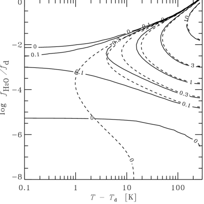
Figure 5: Contour plots of the levels of the constant $6_{16}$–$5_{23}$ maser optical depth $\tau_{\rm m}$ (solid curves) at the plane gas-dust temperature difference – gas-to-dust mass ratio for the following set of parameters $N_{\rm H_{2}}=10^{9}{\rm cm}^{-3}$, $T_{\rm d}=130$ K, $f_{\rm d}=0.01$, and $H=10^{14}$ cm. The dashed curves show the corresponding contours if the de Jong mechanism is not operating (i.e. the photon escape from the slab is neglected and the $K_{2}$ and $L_{2}$ terms in equation (12) are omitted).

3.3 Comparison to the de Jong model

Let us compare the de Jong model to the cold dust model. Using the escape probability approximation, the radiation field is now $\overline{J}=(1-p)S$, where $p$ is the probability for photons to escape without interactions and we neglected here the influence by the dust. The source function is then

$$S=\frac{\epsilon}{\epsilon+p}B.$$ (44)

In the optically thin case, $p\rightarrow 1$, and the source function is then identical to that in the case of the large amount of the cold dust ($B^{\rm d}=0$, see eq. [40]). Thus, in the optically thin limit the de Jong model is similar to the (very) cold dust – hot gas model.

4 Results

4.1 Maser transition $6_{16}$–$5_{23}$

The main results of our calculations for the case of amorphous ice of the size of $0.1\ \mu{\rm m}$ are shown on Figs. 4-6. The dependences of the inversion and the maser optical depth on $N_{\rm H_{2}}$ and $f_{\rm H_{2}O}/f_{\rm d}$ for the fixed dust and gas temperatures are shown in Fig. 4. One sees that when the temperature difference is small (Fig. 4b), the inversion appears in the region where $N_{\rm H_{2}}f_{\rm H_{2}O}/f_{\rm d}\sim 10^{6}$ within two orders of magnitude. The inversion is weak for small $f_{\rm H_{2}O}/f_{\rm d}$. We tested the influence of the de Jong mechanism on the results in this region by neglecting the terms $K_{2}$ and $L_{2}$ in the escape probabilities (12). In that case (dashed curve in Fig. 4b), the inversion is absent there because a higher temperature difference is needed (see eq. [3.2]) to invert the populations.

When $\Delta T$ is larger (see Fig. 4c,d), the inversion becomes larger and the inversion region increases in size, spreading also over to the region with a small water content ($f_{\rm H_{2}O}/f_{\rm d}<10^{-6}$). Here the radiation field is completely dominated by the dust and the inversion depends on the collisional rates defined by $N_{\rm H_{2}}$ only (for the fixed $T$). At lower dust temperature $T_{\rm d}=30$ K (Fig. 4a), the optical depth becomes larger by about 20% comparing with $T_{\rm d}=130$ K (Fig. 4c).

We should point out that the inversion disappears at $N_{\rm H_{2}}\sim 10^{12}{\rm cm}^{-3}$ because of the level thermalization by collisions. This is lower than our analytical estimate (3.2) which neglected many collisional transitions. On the right side the inversion region is bounded by $N_{\rm H_{2}}f_{\rm H_{2}O}/f_{\rm d}<10^{8.5}$ for $T=250$ K, which is very close to our estimate (37).

Let us note that the maximum inversion occurs when the water-to-dust mass ratio $f_{\rm H_{2}O}/f_{\rm d}\sim 10^{5}/N_{\rm H_{2}}$. The maser optical depth, on the other hand, is proportional to $N_{\rm H_{2}O}\Delta n_{\rm m}$ which reaches the maximum at $f_{\rm H_{2}O}/f_{\rm d}\sim 10^{7.5}/N_{\rm H_{2}}$ for $T=250$ K. This corresponds to $N_{\rm H_{2}O}=10^{6.5}f_{\rm d}$. The inversion disappears at $N_{\rm H_{2}O}>10^{7.5}f_{\rm d}$ because the amount of dust (comparing with water) is not sufficient here to produce the inversion. Thus for a given dust content there exists an optimal water concentration that produces the strongest maser. In order to calculate the maser intensity (see eq. [23]) or the brightness temperature in the line center $T_{\rm br}\approx|T_{\rm ex}|\exp(\tau_{\rm m}/\sqrt{\pi})$, one needs to have a rough estimate for the excitation temperature. Because the dependence is linear, the error in that is not important. At the maximum of $\tau_{\rm m}$, the excitation temperature varies between $-10$ and $-100$ K when $T$ varies between 150 and 500 K.

Figure 6: Temperature dependence of the maser optical depth for the same six sets of parameters $(N_{\rm H_{2}},f_{\rm H_{2}O}/f_{\rm d})$ as in Fig. 2. We fixed $H=10^{14}$ cm, $T_{\rm d}=130$ K, $f_{\rm d}=0.01$. The solid curve corresponds to analytical formula (45) with free normalization.

Figure 7: Contours of the constant maser optical depth for the strongest masing transitions of ortho-water for $T_{\rm d}=130$ K, $T=400$ K. Other parameters are the same as in Fig. 4.

Figure 8: Same as in Fig. 7, but for para-water.

On Fig. 5 we present the dependence of $\tau_{\rm m}$ on $f_{\rm H_{2}O}/f_{\rm d}$ and $\Delta T$ for the fixed value of $N_{\rm H_{2}}=10^{9}{\rm cm}^{-3}$. We see that the inversion disappears at large $f_{\rm H_{2}O}/f_{\rm d}$ because the levels are then thermalized at the gas temperature. At small $f_{\rm H_{2}O}/f_{\rm d}$, the medium is optically thin for the line and the dust emission ($\tau_{\rm d}<1$ for most infrared lines at this $N_{\rm H_{2}}$ for $f_{\rm d}=0.01$). Here we also tested the influence of the photon escape from the surface. The dashed curves show the maser optical depth when the escape is neglected. These results show that at small $\Delta T$ the inversion is produced by the de Jong mechanism, while without it the minimum $\Delta T$ to invert the population is about $\sim 1$ K. For small $f_{\rm H_{2}O}/f_{\rm d}$, however, the inversion appears only for $\Delta T>15$ K. At higher $N_{\rm H_{2}}\sim 10^{10}{\rm cm}^{-3}$ this limit is 3.5 K (see dashed curve in Fig. 9) which is very close to the predictions of our four-level model (3.2).

Fig. 6 shows the dependence of the optical depth in the main masing transition $\tau_{\rm m}$ on the gas temperature for the same six sets of parameters $(N_{\rm H_{2}},f_{\rm H_{2}O}/f_{\rm d})$ as in Fig. 2. One sees that in most points the inversion appears when gas temperature exceeds $T_{\rm d}$. At point 4, however, the inversion exists even at smaller $T$. This results from the action of the de Jong mechanism in an optically thin (in line) medium for a small dust content (see also Fig. 3).

The optical depth increases sharply at small $\Delta T$ and saturates at $T\sim 500$ K. This behavior is accurately described by our analytical formula (32). The optical depth is thus proportional to

$$\tau_{\rm m}\propto\left({\rm e}^{-E_{41}/T}-{\rm e}^{-E_{31}/T_{\rm d}}\right)/\sqrt{T},$$ (45)

where the $\sqrt{T}$ factor comes from the Doppler width.

4.2 Other maser transitions

TABLE 1
Ortho-water
masing transitions # Transition $\lambda\ \mu{\rm m}$ 1 $3_{12}\rightarrow 2_{21}$ 260 2 $4_{14}\rightarrow 3_{21}$ 789 3 $4_{23}\rightarrow 3_{30}$ 669 4 $6_{16}\rightarrow 5_{23}$ 13475 5 $5_{32}\rightarrow 4_{41}$ 483 6 $6_{25}\rightarrow 5_{32}$ 227 7 $6_{34}\rightarrow 5_{41}$ 259 8 $6_{43}\rightarrow 5_{50}$ 683 9 $8_{27}\rightarrow 7_{34}$ 231 10 $7_{43}\rightarrow 6_{52}$ 235 11 $7_{52}\rightarrow 6_{61}$ 677 12 $10_{29}\rightarrow 9_{36}$ 933

TABLE 2
Para-water
masing transitions # Transition $\lambda\ \mu{\rm m}$ 1 $3_{13}\rightarrow 2_{02}$ 1636 2 $5_{15}\rightarrow 4_{22}$ 922 3 $5_{24}\rightarrow 4_{31}$ 309 4 $5_{33}\rightarrow 6_{06}$ 632 5 $6_{33}\rightarrow 5_{42}$ 194 6 $7_{26}\rightarrow 6_{33}$ 208 7 $6_{42}\rightarrow 5_{51}$ 637 8 $7_{35}\rightarrow 6_{42}$ 170 9 $7_{44}\rightarrow 6_{51}$ 256 10 $9_{28}\rightarrow 8_{35}$ 331 11 $8_{44}\rightarrow 7_{53}$ 139 12 $8_{53}\rightarrow 7_{62}$ 252

Our simulations show that in addition to the $6_{16}\rightarrow 5_{23}$ maser, there appear many other masers. The strongest masers for ortho-water are listed in Table 1 and for para-water in Table 2. The levels of the constant optical depth are shown in Figs. 7 and 8, respectively. Some of these masers were found in the calculations of Chandra et al. (1984a) and Wallin & Watson (1997). Most of them appear also in models based on the de Jong (1973) mechanism (see also Cooke & Elitzur 1985; Neufeld & Melnick 1991). The $4_{14}\rightarrow 3_{21}$ and $3_{13}\rightarrow 2_{20}$ transitions have been detected in the Orion cloud by Phillips et al. (1980) and Waters et al. (1980). The masing emission in $10_{29}\rightarrow 9_{36}$ line was observed in a wide variety of sources where 1.35 cm maser was detected (Menten, Melnik, & Phillips 1990).

Figure 9: Isolines of the zero inversion of the strongest masing transitions for the same parameters as in Fig. 5. The labels on the contours correspond to the numbering in Table 1. Panel (a) is for $N_{\rm H_{2}}=10^{10}{\rm cm}^{-3}$; (b) corresponds to $N_{\rm H_{2}}=10^{9}{\rm cm}^{-3}$. The inversion of the maser level populations exists on the right side of the corresponding isoline. The left dashed curves show the zero inversion for the $6_{16}\rightarrow 5_{23}$ maser when the de Jong mechanism is turned off.

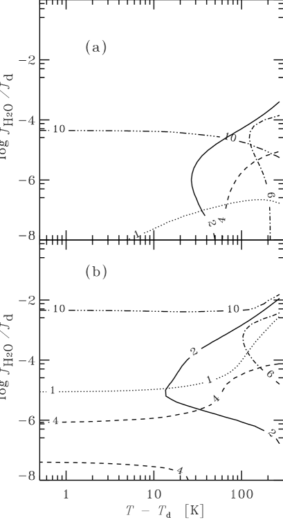
Figure 10: Same as Fig. 9, but for para-water. The labels on the contours correspond to the numbering in Table 2.

We show the isolines of the zero inversion of the level populations as a function of the gas temperature for the fixed $N_{\rm H_{2}}$ in Figs. 9 and 10. The inversion of the level populations appears on the right side from the corresponding curves. We see that the inversion in most of the transitions arises when the difference between the gas and dust temperature is larger than 30–100 K and one does not expect to see a significant signal in other water masing transitions if $\Delta T$ is small. This is related to the fact that the energy separation between the corresponding levels is much larger than that for the $6_{16}\rightarrow 5_{23}$ maser. Many masers also require the water concentration two orders of magnitude smaller than that where the $6_{16}\rightarrow 5_{23}$ and $10_{29}\rightarrow 9_{36}$ masers are strongest (see Figs. 7 and 8). In these respects the cold dust – hot gas model significantly differs from the de Jong model where many masing transitions appear simultaneously.

4.3 Other dust types and sizes

Since the optical properties of the ice in the far infrared spectral range for different grain size $0.01\ \mu{\rm m}\leq a\leq 1\ \mu{\rm m}$ are very similar, the maser strength is almost independent of $a$. The crystalline ice has a stronger peak in $\kappa_{\rm d}$ at $45\ \mu{\rm m}$ and therefore the $6_{16}-5_{23}$ maser optical depth is 30% larger than that for the amorphous ice. We repeated calculations with $0.1\ \mu{\rm m}$ silicate and graphite grains. The optical depth decreases by 15% and 25%, respectively.

We also computed the maser conditions for the mixture of the graphite and SiC dust. We consider the size distribution of the dust grains ${\rm d}n(a)\propto a^{-1.5}{\rm d}a$, which extends from $a_{\min}=0.005\ \mu{\rm m}$ to $a_{\max}=10\ \mu{\rm m}$. To allow easy comparison with the previous results (Collison & Watson 1995; Wallin & Watson 1997), we use an approximation of the results by Laor & Draine (1993, see their Fig. 6) for the dust cross-section. We assume the dust opacity in the form $\kappa_{\rm d}=600(f_{\rm d}/0.01)$ for $\lambda<50\ \mu{\rm m}$ and $\kappa_{\rm d}=600(f_{\rm d}/0.01)(50\ \mu{\rm m}/\lambda)^{2}\ [{\rm cm}^{2}{\rm g}^{-1}]$, for $\lambda>50\ \mu{\rm m}$. The resulting maser optical depth is very similar to that for the crystalline ice.

4.4 Approximating the inversion efficiency for $6_{16}\rightarrow 5_{23}$ maser

The maser luminosity is a function of the optical depth $\tau_{\rm m}$ which depends on the inversion $\Delta n_{\rm m}$. In many astrophysical problems, one would like to make simple estimations of the inversion and optical depth not repeating cumbersome calculations of the water molecular level populations. Thus one would like to have simple analytical approximate formulae for this purpose.

It is possible to design a formula for the inversion that describes it with an error of a factor of two using the four-level model from Sect. 3. We can further simplify the model by assuming that the upper masing level $6_{16}$ is populated directly from the $4_{14}$ level. We then arrive to a system of two equations, each corresponding to the two-level model. We now can introduce a pseudo-transition $1\rightarrow 4$, and prescribe to it some collisional and radiative rates.

We propose the following formula to compute the inversion:

$$\Delta n_{\rm m}=\frac{n_{1}}{g_{1}}\left(\frac{S_{41}}{1+S_{41}}-\frac{S_{31}}{1+S_{31}}\right).$$ (46)

The population at the lower level 1 is given by the following expression

$$\frac{n_{1}}{g_{1}}=0.75U^{-1}_{\rm part}\exp(-289/T),$$ (47)

where, based on the results of simulations, we can approximate the partition function in the range $10<T<500$ K as

$$U_{\rm part}=2.86[1+(T/42)^{1.4}].$$ (48)

Approximating the dependence of the collisional rate on the gas temperature by a power-law, we get the ratio

$$\epsilon_{31}=0.033\frac{N_{\rm H_{2}}}{10^{10}}\left(\frac{T}{100}\right)^{0.92}\left(1-\exp[-319/T]\right).$$ (49)

The dust influence is parametrized by $\beta$:

$$\beta_{31}=2\times 10^{-6}(T/100)^{1/2}(f_{\rm H_{2}O}/f_{\rm d})^{-1},$$ (50)

and $\delta_{31}$ is computed using equation (14). We now can assume that the $4\rightarrow 1$ transition is characterized by $\epsilon_{41}=1.1\epsilon_{31}$ and $\beta_{41}=0.6\beta_{31}$. The source functions are found from equation (29). These formulae give a rather good agreement with the results of numerical simulations (within a factor of two).

5 Conclusions

We consider the cold dust – hot gas mechanism of pumping of the water masers. To obtain the inversion of the maser level populations we take into account the first 45 rotational levels of ortho- and para-H₂O molecules and all possible collisional and radiative transitions between them. In the case of the large optical depth in the main pumping lines and the unsaturated masers, the radiative transfer problem can be significantly simplified, allowing us to investigate the maser efficiency for the set of the main parameters, such as the hydrogen concentration, the gas-to-dust mass ratio and the gas temperature.

As it was suggested by Deguchi (1981), the pumping cycle $4_{14}\rightarrow 5_{05}\rightarrow 6_{16}\rightarrow 5_{23}\rightarrow 4_{14}$ mainly determines the inversion of the $6_{16}-5_{23}$ maser levels populations. We use this four-level model for the analysis of our numerical results. We also suggest approximate formulae for the dependence of the inversion on the hydrogen concentration, the gas-to-dust mass ratio and the gas and dust temperatures, that could be used for modeling the astrophysical sources. We find that the inversion is the largest when the water-to-dust mass ratio is $f_{\rm H_{2}O}/f_{\rm d}\sim 10^{5}/N_{\rm H_{2}}$, and the maser optical depth is the largest when $N_{\rm H_{2}O}\sim(10^{6}\div 10^{7})f_{\rm d}$.

The inversion of the maser level populations as a function of the same parameters is calculated in the case of the amorphous and crystalline ice, silicate as well as graphite dust. The results of these calculations are very similar. Because the inversion depends on the dust mass density, our results can be applied to any size distribution of the dust particles.

Our analysis shows that in the optically thick environments the inversion in the $6_{16}\rightarrow 5_{23}$ transition appears when the gas is just $\sim 1$ K hotter than the dust, while most of other transitions start to be inverted at much larger $\Delta T\sim 30-100$ K. Most of them require also smaller water-to-dust mass ratio $f_{\rm H_{2}O}/f_{\rm d}$. This is very different from the predictions of the de Jong model where many transitions are inverted simultaneously. If the cold dust – hot gas model is the correct one, the relative ratios of the luminosities in different masing transitions could provide constraints on the gas and dust temperatures, water-to-dust mass ratio, and hydrogen concentration.