Observational constraints on dark energy model

Abstract

The recent observations support that our Universe is flat and expanding with acceleration. We analyze a general class of quintessence models by using the recent type Ia supernova and the first year Wilkinson Microwave Anisotropy Probe (WMAP) observations. For a flat universe dominated by a dark energy with constant $\omega$ which is a special case of the general model, we find that $\Omega_{\rm m0}=0.30^{+0.06}_{-0.08}$ and $\omega_{\rm Q}\leq-0.82$, and the turnaround redshift $z_{\rm T}$ when the universe switched from the deceleration phase to the acceleration phase is $z_{\rm T}=0.65$. For the general model, we find that $\Omega_{\rm m0}\sim 0.3$, $\omega_{\rm Q0}\sim-1.0$, $\beta\sim 0.5$ and $z_{\rm T}\sim 0.67$. A model independent polynomial parameterization of dark energy is also considered, the best fit model gives $\Omega_{\rm m0}=0.40\pm 0.14$, $\omega_{\rm Q0}=-1.4$ and $z_{\rm T}=0.37$.

1 Introduction

The type Ia supernova (SN Ia) observations indicate that the expansion of the Universe is speeding up rather than slowing down [1]-[4]. The measurement of the anisotropy of the cosmic microwave background (CMB) favors a flat universe [5, 6, 7]. The observation of type Ia supernova SN 1997ff at $z\sim 1.7$ also provides the evidence that the Universe is in the acceleration phase and was in the deceleration phase in the past [4, 8]. The transition from the deceleration phase to the acceleration phase happened around the redshift $z_{\rm T}\sim 0.4$ [4, 9]. In this paper, we use the notation $z_{\rm T}$ for the transition redshift. A new component with negative pressure widely referred as dark energy is usually introduced to explain the accelerating expansion. The simplest form of dark energy is the cosmological constant with the equation of state parameter $\omega_{\rm\Lambda}=-1$. One easily generalizes the cosmological constant model to dynamical cosmological constant models such as the dark energy model with negative constant equation of state parameter $-1\leq\omega_{\rm Q}<-1/3$ and the holographic dark energy models [10]. If we remove the null energy condition restriction $\omega_{\rm Q}\geq-1$ to allow supernegative $\omega_{\rm Q}<-1$, then we have the phantom energy models [11]. More exotic equation of state is also possible, such as the Chaplygin gas model with the equation of state $p=-A/\rho$ and the generalized Chaplygin gas model with the equation of state $p=-A/\rho^{\alpha}$ [12]. In general, a scalar field $Q$ that slowly evolves down its potential $V(Q)$ takes the role of a dynamical cosmological constant. The scalar field $Q$ is also called the quintessence field [13]-[20]. The energy density of the quintessence field must remain very small compared with that of radiation or matter at early epoches and evolves in a way that it started to dominate the universe around the redshift $0.4$. Instead of the quintessence field with the usual kinetic term $\dot{Q}^{2}/2$, tachyon field as dark energy was also proposed [21]. The tachyon models have the accelerated phase followed by the decelerated phase.

Although most dark energy models are consistent with current observations, the nature of dark energy is still mysterious. Therefore it is also possible that the observations show a sign of the breakdown of the standard cosmology. Some alternative models to dark energy models were proposed along this line of reasoning. These models are motivated by extra dimensions. In these models, the usual Friedmann equation $H^{2}=8\pi G\rho/3$ is modified to a general form $H^{2}=g(\rho)$ and the universe is composed of the ordinary matter only [22]-[29]. In other words, the dark energy component is unnecessary.

In this paper, I first use the 58 SN Ia data in Ref. raknop03, the 186 SN Ia data in Ref. riess and WMAP data [7] to constrain the parameter space of a general class of quintessence models discussed in Ref. gong02. In that model, a general relation between the potential energy and the kinetic energy of the quintessence field was proposed. As we know, the average kinetic energy is the same as the average potential energy for a point mass in a harmonic oscillator. For a stable, self-gravitating, spherical distribution of equal mass objects, the total kinetic energy of the objects is equal to minus 1/2 times the total gravitational potential energy. Therefore, the physics of dark energy may be determined if the relationship between the potential energy and the kinetic energy is known. Then I consider three different model independent parameterizations of $\omega_{\rm Q}$ to find out some properties of dark energy. After we determine the parameters in these models, the transition redshift $z_{\rm T}$ is obtained. The paper is organized as follows. After a brief introduction in section 1, the general class of models is reviewed in section 2. In section 3, I discuss the methodology used in this paper. In section 4, I give the main fitting results. In section 5, I conclude the paper by using a model independent analysis and compare the results with those in the literature.

2 Model Review

For a spatially flat, isotropic and homogeneous universe with both an ordinary pressureless dust matter and a minimally coupled scalar field $Q$ source, the Friedmann equations are

$$H^{2}\equiv\left({\dot{a}\over a}\right)^{2}={8\pi G\over 3}(\rho_{\rm m}+\rho_{\rm Q}),$$ (1)

$${\ddot{a}\over a}=-{4\pi G\over 3}(\rho_{\rm m}+\rho_{\rm Q}+3p_{\rm Q}),$$ (2)

$$\ddot{Q}+3H\dot{Q}+V^{\prime}(Q)=0,$$ (3)

where dot means derivative with respect to time, $\rho_{\rm m}=\rho_{\rm m0}(a_{0}/a)^{3}$ is the matter energy density, a subscript 0 means the value of the variable at present time, $\rho_{\rm Q}=\dot{Q}^{2}/2+V(Q)$, $p_{\rm Q}=\dot{Q}^{2}/2-V(Q)$, $V^{\prime}(Q)=dV(Q)/dQ$ and $V(Q)$ is the potential of the quintessence field. In Ref. gong02, a general relationship

$$V(Q)=\beta\dot{Q}^{2}+C,$$ (4)

was proposed instead of assuming a particular potential for the quintessence field or a particular form of the scale factor, where $\beta$ and $C$ are constants. Note that the above equation (4) is a constraint equation, one should not just substitute the above equation into the Lagrangian and thinks that the model is equivalent to a $1/2+\beta$ kinetic term plus a cosmological constant term $C$. The above general potential includes the hyperbolic potential and the double exponential potential. In terms of $\rho_{\rm Q0}$ and $\omega_{\rm Q0}$, we have

$$C = \left[{1\over 2}-\beta-\left({1\over 2}+\beta\right)\omega_{\rm Q0}\right]\rho_{\rm Q0},$$ (5)

$$\rho_{\rm Q} = (1/2+\beta)(1+\omega_{\rm Q0})\rho_{\rm Q0}\left({a_{0}\over a}\right)^{6/(2\beta+1)}+\left[{1\over 2}-\beta-\left({1\over 2}+\beta\right)\omega_{\rm Q0}\right]\rho_{\rm Q0},$$ (6)

$$p_{\rm Q} = (1/2-\beta)(1+\omega_{\rm Q0})\rho_{\rm Q0}\left({a_{0}\over a}\right)^{6/(2\beta+1)}-\left[{1\over 2}-\beta-\left({1\over 2}+\beta\right)\omega_{\rm Q0}\right]\rho_{\rm Q0},$$ (7)

$$H^{2} = {8\pi G\over 3}\left\{\rho_{\rm m0}\left(a_{0}\over a\right)^{3}+(1/2+\beta)(1+\omega_{\rm Q0})\rho_{\rm Q0}\left({a_{0}\over a}\right)^{6/(2\beta+1)}+C\right\}.$$ (8)

To make the quintessence field sub-dominated during early times, we require that $\beta\geq 0.5$. The transition from deceleration to acceleration happens when the deceleration parameter $q=-\ddot{a}H^{2}/a=0$. From equations (2), (6) and (7), in terms of the redshift parameter $1+z=a_{0}/a$, we have

$$(1+z_{\rm T})^{3}+2(1-\beta)(1+\omega_{\rm Q0}){\rho_{\rm Q0}\over\rho_{\rm m0}}(1+z_{\rm T})^{6/(2\beta+1)}-[1-2\beta-(1+2\beta)\omega_{\rm Q0}]{\rho_{\rm Q0}\over\rho_{\rm m0}}=0.$$ (9)

This equation gives a relationship between $\omega_{\rm Q0}$ and $\Omega_{\rm Q0}$. Now let us turn our attention to two special cases.

Case 1: $C=0$, the equation of state of the scalar field is a constant, $\omega_{\rm Q}=(1/2-\beta)/(1/2+\beta)$. The potential is [17, 18]

$$V(Q)=A[\sinh k(Q/\alpha+B)]^{-\alpha},$$

where $\alpha=2/(\beta-1/2)$, $k^{2}=48\pi G/(2\beta+1)$, $A^{\beta-1/2}=(1/2+\beta)C_{2}^{2\beta+1}\beta^{\beta-1/2}/(\rho_{\rm m0}a^{3}_{0})$ and $B$ is an arbitrary integration constant.

Case 2: $\beta=1/2$, the pressure of the scalar field becomes a constant $p_{\rm Q}=-C=\omega_{\rm Q0}\rho_{\rm Q0}$ and the potential is the double exponential potential [19]

$$V(Q)={A^{2}\over 8}[\exp(2\alpha Q)+\exp(-2\alpha Q)]+{\alpha^{2}A^{2}\over 6\pi G}-{A^{2}\over 4}.$$

The constant pressure model is equivalent to an ordinary matter with effective matter content $\Omega^{\rm eff}_{\rm m0}=(1+\omega_{\rm Q0})\Omega_{\rm Q0}+\Omega_{\rm m0}$ plus a cosmological constant $\rho_{\Lambda}=-\omega_{\rm Q0}\rho_{\rm Q0}$.

3 Methodology

In order to use the WMAP result, one usually parameterizes the location of the $m$-th peak of CMB power spectrum as [30]

$$l_{m}=(m-\phi_{m})l_{\rm A},$$

where the acoustic scale $l_{\rm A}$ is

$$l_{\rm A}={\pi\over\bar{c_{\rm s}}}{\tau_{0}-\tau_{\rm ls}\over\tau_{\rm ls}}={\pi\over\bar{c_{\rm s}}}{\int^{z_{\rm ls}}_{0}dz/\sqrt{g(z)}\over\int^{\infty}_{z_{\rm ls}}dz/\sqrt{g(z)}},$$ (10)

the conformal time at the last scattering $\tau_{\rm ls}$ and at today $\tau_{0}$ are

$$\tau_{\rm ls} = \int^{\tau_{\rm ls}}_{0}d\tau=\int^{\infty}_{z_{\rm ls}}{dz\over a_{0}H_{0}\sqrt{g(z)}},$$ (11)

$$\tau_{0} = \int^{\tau_{0}}_{0}d\tau=\int^{\infty}_{0}{dz\over a_{0}H_{0}\sqrt{g(z)}},$$ (12)

$$g(z) = \Omega_{\rm m0}(1+z)^{3}+\Omega_{\rm r0}(1+z)^{4}+(1/2+\beta)(1+\omega_{\rm Q0})\Omega_{\rm Q0}(1+z)^{6/(2\beta+1)}$$ (13)

$$+\left[{1\over 2}-\beta-\left({1\over 2}+\beta\right)\omega_{\rm Q0}\right]\Omega_{\rm Q0},$$

$\Omega_{\rm r0}=8.35\times 10^{-5}$ is the current radiation component and $z_{\rm ls}=1089\pm 1$ [6]. The difficulty of this method is that there are several undetermined parameters, such as $\phi_{m}$ and $\bar{c}_{s}$. Instead, we use the CMB shift parameter $\mathcal{R}\equiv\Omega_{\rm m0}^{1/2}a_{0}H_{0}(\tau_{0}-\tau_{\rm ls})=1.716\pm 0.062$ [31] to constrain the model.

The luminosity distance $d_{\rm L}$ is defined as

$$d_{\rm L}(z)=a_{0}c(1+z)\int^{t_{0}}_{\rm t}{dt^{\prime}\over a(t^{\prime})}=c{1+z\over H_{0}}\int^{z}_{0}du[g(u)]^{-1/2}.$$ (14)

The apparent magnitude redshift relation becomes

$$m(z) = M+5\log_{10}d_{\rm L}(z)+25=\mathcal{M}+5\log_{10}\mathcal{D}_{\rm L}(z)$$ (15)

$$= \mathcal{M}+5\log_{10}\left[c(1+z)\int^{z}_{0}du[g(u)]^{-1/2}\right],$$

where $\mathcal{D}_{\rm L}(z)=H_{0}d_{\rm L}(z)$ is the ”Hubble-constant-free” luminosity distance, $M$ is the absolute peak magnitude and $\mathcal{M}=M-5\log_{10}H_{0}+25$. $\mathcal{M}$ can be determined from the low redshift limit at where $\mathcal{D}_{\rm L}(z)=z$. We use the 54 SNe Ia data with both the stretch correction and the host-galaxy extinction correction, i.e., the fit 3 supernova data in Ref. raknop03 (we refer the data as Knop sample), and the 186 SNe Ia data in Ref. riess (we refer the data as Riess sample) to constrain the model. The parameters in the model are determined using a $\chi^{2}$-minimization procedure based on MINUIT code. There are four parameters in the fit: the current mass density $\Omega_{\rm m0}$, the current dark energy equation of state parameter $\omega_{\rm Q0}$, the constant $\beta$ as well as the nuisance parameter $\mathcal{M}$. The range of parameter space is $\Omega_{\rm m0}=[0,\ 1]$ and $\omega_{\rm Q0}=(-1,\ 0]$.

4 Results

For the dark energy model with constant $\omega_{\rm Q}$, i.e., the model with $C=0$, the best fit parameters to the 54 knop sample are $\Omega_{\rm m0}=[0,\ 0.46]$ centered at 0.30 and $\omega_{\rm Q}=(-1.0,\ -0.44]$ centered at almost $-1.0$ with $\chi^{2}=45.6$ at 68% confidence level. The best fit parameters to the 157 Riess gold sample are $\Omega_{\rm m0}=[0.19,\ 0.37]$ centered at 0.31 and $\omega_{\rm Q}=(-1,\ -0.75]$ centered at almost $-1.0$ with $\chi^{2}=177.1$ at 68% confidence level. The best fit parameters to the 186 Riess gold and silver sample are $\Omega_{\rm m0}=[0.22,\ 0.36]$ centered at 0.30 and $\omega_{\rm Q}=(-1,\ -0.81]$ centered at almost $-1.0$ with $\chi^{2}=232.3$ at 68% confidence level. The best fit parameters to the Riess gold sample and WMAP data combined are $\Omega_{\rm m0}=[0.22,\ 0.36]$ centered at 0.30 and $\omega_{\rm Q}=(-1.0,\ -0.81]$ centered at almost $-1.0$ with $\chi^{2}=177.3$ at 68% confidence level. The best fit parameters to the Riess gold and silver sample and WMAP data combined are $\Omega_{\rm m0}=[0.23,\ 0.35]$ centered at 0.30 and $\omega_{\rm Q}=(-1.0,\ -0.84]$ centered at almost $-1.0$ with $\chi^{2}=232.4$ at 68% confidence level. From the above results, it is shown that the addition of Riess silver data give almost the same results as those from Riess gold sample only. Therefore, we will use Riess gold sample only in the following discussion. The confidence regions of $\Omega_{\rm m0}$ and $\omega_{\rm Q}$ are shown in figure 1.

$\begin{array}[]{cc}\epsfbox{cwknop.eps}&\epsfbox{cwriess1.eps}\\ \epsfbox{cwriess2.eps}&\epsfbox{cwriessmap1.eps}\end{array}$

Figure 1: The confidence contours of $\Omega_{\rm m0}$ and $\omega_{\rm Q}$ for the $C=0$ model. The left upper panel is the 68%, 95% and 99% confidence regions fitted from Knop sample. The right upper panel is the 68%, 95%, 99% confidence regions fitted from Riess gold sample, the left lower panel is the 68%, 95% and 99% confidence regions fitted from Riess gold and silver sample. The right lower panel is the 68%, 95%, 99% confidence regions fitted from Riess gold sample and WMAP data.

For the general model $C\neq 0$, we first analyze the special constant pressure model $\beta=1/2$ which is equivalent to the $\Lambda$-CDM mdoel. The best fits to the 54 Knop sample are $\Omega_{\rm m0}=[0,\ 0.46]$ centered at almost zero and $\omega_{\rm Q0}=(-1,\ -0.54]$ centered at $-0.71$ with $\chi^{2}=45.6$ at 68% confidence level. The best fits to the 157 Riess gold sample are: $0\leq\Omega_{\rm m0}\leq 0.37$ and $-1<\omega_{\rm Q0}\leq-0.63$ at 68% confidence level with $\chi^{2}=177.1$. Note that the effective $\Omega_{\rm m0}\sim 0.3$ although the best fit $\Omega_{\rm m0}$ is almost zero. The best fits to the 157 Riess gold sample and WMAP data combined are: $0.25\leq\Omega_{\rm m0}\leq 0.35$ and $-1<\omega_{\rm Q0}\leq-0.93$ with $\chi^{2}=177.1$ at 68% confidence level. The confidence regions of $\Omega_{\rm m0}$ and $\omega_{\rm Q0}$ are shown in figures 2 and 3.

$\begin{array}[]{cc}\epsfbox{quinknop.eps}&\epsfbox{quinriess.eps}\end{array}$

Figure 2: The 68%, 95% and 99% confidence contours of $\Omega_{\rm m0}$ and $\omega_{\rm Q0}$ for $\beta=1/2$. The left panel shows fits to Knop sample and the right panel shows fits to Riess gold sample.

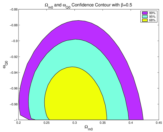
Figure 3: The 68%, 95% and 99% confidence contours of $\Omega_{\rm m0}$ and $\omega_{\rm Q0}$ for $\beta=1/2$ with Riess gold sample and WMAP data.

For the general model, the range of parameter space is $\Omega_{\rm m0}=[0,\ 1]$, $\omega_{\rm Q0}=(-1,\ 0]$ and $\beta\geq 0.5$. The best fits to the 54 Knop sample are: $0\leq\Omega_{\rm m0}\leq 0.50$, $-1<\omega_{\rm Q0}\leq-0.23$ and $\beta$ varies in a big range with $\chi^{2}=45.6$ at 68% confidence level. The best fits to the 157 Riess gold sample are: $0\leq\Omega_{\rm m0}\leq 0.38$, $-1<\omega_{\rm Q0}\leq-0.57$ and $\beta$ varies in a big range with $\chi^{2}=177.1$ at 68% confidence level. The best fits to the 157 Riess gold sample and WMAP data combined are: $0.21\leq\Omega_{\rm m0}\leq 0.37$, $-1.0<\omega_{\rm Q0}\leq-0.75$ and $\beta\geq 0.5$ with $\chi^{2}=177.1$ at 68% confidence level. From the above results, we see that the best fit model tends to be the $\Lambda$-CDM model with $\Omega_{\rm m0}\sim 0.3$.

$\begin{array}[]{cc}\epsfbox{rhowqz1b.eps}&\epsfbox{rhowqz2b.eps}\end{array}$

Figure 4: The best supernova and WMAP data fits to the polynomial model and linear model. The left panel shows Riess gold sample and WMAP data fits to the two parameter polynomial model, the light black lines are for $\Omega_{\rm Q}$ and the dark balck lines for $\omega_{\rm Q}$, the solid lines are from the best fit. The right panel shows Riess gold sample and WMAP data fits to the two parameter linear model of $\omega_{\rm Q}$, the solid lines are from the best fit, the light black lines are for the linear model and the dark black lines are for the stable model. The dashed lines define the 1$\sigma$ boundaries.

5 Model-independent Results

To construct a model independent result, we first parameterize the dark energy density by two parameters [32], $\Omega_{\rm Q}(z)=A_{0}+A_{1}(1+z)+A_{2}(1+z)^{2}$, here $\Omega_{\rm Q}(z)=8\pi G\rho_{\rm Q}(z)/(3H^{2}_{0})$ and $A_{0}=1-\Omega_{\rm m0}-\Omega_{\rm r0}-A_{1}-A_{2}$. The relationship between the dark energy state of equation parameter $\omega_{\rm Q}$ and the redshift is

$$\omega_{\rm Q}={1+z\over 3}{A_{1}+2A_{2}(1+z)\over A_{0}+A_{1}(1+z)+A_{2}(1+z)^{2}}-1.$$

With the above parameteriaztion, we find that $\Omega_{\rm Q}\ll\Omega_{m}$ and $\omega_{\rm Q}\approx-1/3$ when $z\gg 1$. The best fit parameters to Riess gold sample and WMAP data are $\Omega_{\rm m0}=0.40\pm 0.14$, $A_{1}=-3.6^{+3.8}_{-4.6}$ and $A_{2}=1.23^{+1.74}_{-1.23}$ with $\chi^{2}=174.3$. By using the best fit parameters, we find that $\omega_{\rm Q0}=-1.4$ and $z_{\rm T}=0.37$. Then we consider the commonly used two parameter linear model $\omega_{\rm Q}(z)=\omega_{0}+\omega_{1}(1+z)$. The Riess gold sample and WMAP data give that $\Omega_{\rm m0}=0.49^{+0.09}_{-0.20}$, $\omega_{0}=-2.57^{+1.58}_{-5.18}$ and $\omega_{1}=0.16^{+0.53}_{-0.16}$ with $\chi^{2}=173.7$. Combining the best fit parameters, it is found that $\omega_{\rm Q0}=-2.41$ and $z_{\rm T}=0.29$. Because the above linear model is divergent as $z\gg 1$, so we next consider a more stable prarmeterization of $\omega_{\rm Q}(z)=\omega_{0}+\omega_{a}z/(1+z)$ [33]. By using this parameterization, we find that the best fit parameters to Riess gold sample and WMAP data are $\Omega_{\rm m0}=0.47^{+0.10}_{-0.19}$, $\omega_{0}=-2.5^{+1.5}_{-4.9}$ and $\omega_{a}=3.2^{+6.6}_{-3.2}$ with $\chi^{2}=173.5$. Therefore the turnaround redshift is $z_{\rm T}=0.28$ and $\omega_{\rm Q0}=-2.5$. Note that the cosmological constant model $\omega_{0}=-1$ and $\omega_{a}=0$ is at the boundary of the $1\sigma$ parameter space. However, the dark energy term became the dominant term when $z\gg 1$ since $\omega_{0}+\omega_{a}=0.7$. Therefore, we use the results from the polynomial parameterization only. The evolutions of $\Omega_{\rm Q}(z)$ and $\omega_{\rm Q}(z)$ with redshift are shown in figure 4.

For the model independent second order polynomial parameterization, we find that $\Omega_{\rm m0}=0.40\pm 0.14$, $\omega_{\rm Q0}=-1.4$ and $z_{\rm T}=0.37$. Alam, Sahni and Starobinsky obtained $\Omega_{\rm m0}=0.385$ and $z_{\rm T}=0.39\pm 0.03$ in a similar analysis [32]. Tegmark et al. found that $\Omega_{\rm m0}\approx 0.30\pm 0.04$ by using the WMAP data in combination with the Sloan Digital Sky Survey (SDSS) data [34]. More recently, Riess et al. showed that $z_{\rm T}=0.46\pm 0.13$ from the two parameter linear model by using SNe Ia data only with the assumption that $\Omega_{\rm m0}=0.27\pm 0.04$ [4]. The above results are consistent with each other. For a flat universe with constant $\omega_{\rm Q}$, we find that $\Omega_{\rm m0}=0.30^{+0.06}_{-0.08}$ and $\omega_{\rm Q}\leq-0.82$. The result is consistent with our model independent results and that in Refs. raknop03,riess,weller. With those parameter values, we find that the turnaround redshift $0.47\leq z_{\rm T}\leq 0.95$. For the constant pressure model $\beta=1/2$, the best fits to the combined supernova and WMAP data are $\Omega_{\rm m0}=0.298$ and $\omega_{\rm Q0}=-0.985$ which result in $z_{\rm T}=0.65$. The best parameter fits to the combined supernova and WMAP data for the general model analyzed in this paper are $\Omega_{\rm m0}\sim 0.3$, $\omega_{\rm Q0}\sim-1.0$ and $\beta\sim 0.5$. The turnaround redshfit is $z_{\rm T}\sim 0.67$. These results are consistent with the observations. In conclusion, it is shown that the general model in Ref. gong02 is consistent with current observations and the model effectively tends to be the $\Lambda$-CDM model. Furthermore, our model independent results support the conclusion of dark energy metamorphosis obtained in Ref.  alam.

References

- [1] S. Perlmutter et al., Nature 391, 51 (1998); Astrophys. J. 517, 565 (1999); P.M. Garnavich et al., Astrophys. J. Lett. 493, L53 (1998); A.G. Riess et al., Astron. J. 116, 1009 (1998).
- [2] J.L. Tonry et al., Astrophys. J. 594, 1 (2003); B.J. Barris et al., ibid. 602, 571 (2004)
- [3] R.A. Knop et al., Astrophys. J. 598, 102 (2003);.
- [4] A.G. Riess et al., Astrophys. J. 607, 665 (2004).
- [5] P. de Bernardis et al., Nature 404, 955 (2000); S. Hanany et al., Astrophys. J. Lett. 545, L5 ( 2000).
- [6] C.L. Bennett et al., Astrophys. J. Supp. Ser. 148, 1 (2003).
- [7] D.N. Spergel et al., Astrophys. J. Supp. Ser. 148, 175 (2003).
- [8] A.G. Riess, Astrophys. J. 560, 49 (2001).
- [9] M.S. Turner and A.G. Riess, Astrophys. J. 569, 18 (2002); R.A. Daly and S.G. Djorgovski, ibid. 597, 9 (2003); 612, 652 (2004).
- [10] A. Cohen, D. Kaplan and A. Nelson, Phys. Rev. Lett. 82, 4971 (1999); S.D.H. Hsu, Phys. Lett. B594, 13 (2004); R. Horvat, Phys. Rev. D70, 087301 (2004); M. Li, Phys. Lett. B603, 1 (2004); Q.G. Huang and Y. Gong, J. Cosm. Astropart. Phys. 0408, 006 (2004); Y. Gong, Phys. Rev. D70, 064029 (2004).
- [11] R.R. Caldwell, Phys. Lett. B545, 23 (2002); A. Melchiorri, I. Mersini, C.J. Odman and M. Trodden, Phys. Rev. D68, 043509 (2003); G.W. Gibbons, hep-th/0302199; S.M. Carroll, M. Hoffman and M. Trodden, Phys. Rev. D68, 023509 (2003); J.G. Hao and X.Z. Li, Phys. Rev. D67, 107303 (2003); D70, 043529 (2004); Phys. Lett. B606, 7 (2005); P. Singh, M. Sami and N. Dadhich, Phys. Rev. D68, 023522 (2003); J.S. Alcaniz, Phys. Rev. D69, 083521 (2004); M. Kaplinghat and S. Bridle, astro-ph/0312430.
- [12] A. Kamenshchik, U. Moschella and V. Pasquier, Phys. Lett. B511, 265 (2001); N. Bilic, G. Tupper and R.D. Viollier, ibid. B535, 17 (2002); M.C. Bento, O. Bertolami and A.A. Sen, Phys. Rev. D66, 043507 (2002); D. Carturan and F. Finelli, ibid. D68, 103501 (2003); J.V. Cunha, J.S. Alcaniz and J.A.S. Lima, ibid. D69, 083501 (2004); L. Amendola, F. Finelli, C. Burigana and D. Carturan, J. Cosm. Astropart. Phys. 0307, 005 (2003).
- [13] R.R. Caldwell, R. Dave and P.J. Steinhardt, Phys. Rev. Lett. 80, 1582 (1998); I. Zlatev, L. Wang and P.J. Steinhardt, ibid. 82, 896 (1999).
- [14] P.G. Ferreira and M. Joyce, Phys. Rev. Lett. 79, 4740 (1997); P.G. Ferreira and M. Joyce, Phys. Rev. D58, 023503 (1998).
- [15] B. Ratra and P.J.E. Peebles, Phys. Rev. D37, 3406 (1988); C. Wetterich, Nucl. Phys. B302, 668 (1988).
- [16] S. Perlmutter, M.S. Turner and M. White, Phys. Rev. Lett. 83, 670 (1999).
- [17] V. Sahni and A.A. Starobinsky, Int. J. Mod. Phys. D9, 373 (2000); C. Rubano and J.D. Barrow, Phys. Rev. D64, 127301 (2001); V.B. Johri, Class. Quantum Grav. 19, 5959 (2001).
- [18] L.A. Ureña-López and T. Matos, Phys. Rev. D62, 081302 (2000); E. Di Pietro and J. Demaret, Int. J. Mod. Phys. D10, 231 (2001).
- [19] A.A. Sen and S. Sethi, Phys. Lett. B532, 159 (2002).
- [20] Y. Gong, Class. Quantum Grav. 19, 4537 (2002).
- [21] C. Armendariz-Picon, T. Damour and V. Mukhanov, Phys. Lett. B458, 209 (1999); T. Padmanabhan and T.R. Choudhury, Phys. Rev. D66, 081301 (2002); J.S. Bagla, H.K. Jassal and T. Padmanabhan, ibid. D67, 063504 (2003); T. Padmanabhan, Phys. Rep. 380, 235 (2003); T. Padmanabhan and T.R. Choudhury, Mon. Not. Roy. Astron. Soc. 344, 823 (2003).
- [22] K. Freese and M. Lewis, Phys.Lett. B540, 1 (2002); K. Freese, Nucl. Phys. Suppl. 124, 50 (2003).
- [23] P. Gondolo and K. Freese, Phys. Rev. D68, 063509 (2003).
- [24] S. Sen and A.A. Sen, Astrophys. J. 588, 1 (2003) ; A. A. Sen and S. Sen, Phys. Rev. D68, 023513 (2003).
- [25] Z.H. Zhu and M. Fujimoto, Astrophys. J. 581, 1 (2002); 585, 52 (2003); 602, 12 (2004); Z.H. Zhu, M. Fujimoto and X.T. He, ibid. 603, 365 (2004).
- [26] Y. Wang, K. Freese, P. Gondolo and M. Lewis, Astrophys. J. 594, 25 (2003).
- [27] T. Multamaki, E. Gaztanaga and M. Manera, Mon. Not. Roy. Astron. Soc. 344, 761 (2003).
- [28] W.J. Frith, Mon. Not. Roy. Astron. Soc. 348, 916 (2004).
- [29] Y. Gong and C.K. Duan, Class. Quantum Grav. 21, 3655 (2004); Mon. Not. Roy. Astron. Soc. 352, 847 (2004); Y. Gong, X.M. Chen and C.K. Duan, Mod. Phys. Lett. A19, 1933 (2004).
- [30] W. Hu, M. Fukugita, M. Zaldarriaga and M. Tegmark, Astrophys. J. 549, 669 (2001); M. Doran, M. Lilley, J. Schwindt and C. Wetterich, ibid. 559, 501 (2001); M. Doran, M. Lilley and C. Wetterich, Phys. Lett. B528, 175 (2002); M. Doran and M. Lilley, Mon. Not. Roy. Astron. Soc. 330, 965 (2002).
- [31] J.R. Bond, G. Efstathiou and M. Tegmark, Mon. Not. Roy. Astron. Soc. 291, L33 (1997); A. Melchiorri, L. Mersini, C.J. Ödman and M. Trodden, Phys. Rev. D68, 043509 (2003); Y. Wang and P. Mukherjee, Astrophys. J. 606, 654 (2004); Y. Wang and M. Tegmark, Phys. Rev. Lett. 92, 241302 (2004).
- [32] U. Alam, V. Sahni, T.D. Saini and A.A. Starobinsky, Mon. Not. Roy. Astron. Soc. 354, 275 (2004); U. Alam, V. Sahni and A.A. Starobinsky, J. Cosm. Astropart. Phys. 0406, 008 (2004); Y. Gong, Class. Quantum Grav., in press, astro-ph/0405446.
- [33] M. Chevallier and D. Polarski, Int. J. Mode. Phys. D10, 213 (2001); E.V. Linder, Phys. Rev. Lett. 90, 91301 (2003).
- [34] M. Tegmark et al., Phys. Rev. D69, 103501 (2004).
- [35] J. Weller and A.M. Lewis, Mon. Not. Roy. Astron. Soc. 346, 987 (2003); P. Schuecker et al., Astron. Astrophys. 402, 53 (2003).