A Search for Kinematic Evidence of Radial Gas Flows in Spiral Galaxies

Abstract

CO and H I velocity fields of seven nearby spiral galaxies, derived from radio-interferometric observations, are decomposed into Fourier components whose radial variation is used to search for evidence of radial gas flows. Additional information provided by optical or near-infrared isophotes is also considered, including the relationship between the morphological and kinematic position angles. To assist in interpreting the data, we present detailed modeling that demonstrates the effects of bar streaming, inflow, and a warp on the observed Fourier components. We find in all of the galaxies evidence for either elliptical streaming or a warped disk over some range in radius, with deviations from pure circular rotation at the level of $\sim$20–60 km s^-1. Evidence for kinematic warps is observed in several cases well inside $R_{25}$. No unambiguous evidence for radial inflows is seen in any of the seven galaxies, and we are able to place an upper limit of $\sim$5–10 km s^-1 (3–5% of the circular speed) on the magnitude of any radial inflow in the inner regions of NGC 4414, 5033 and 5055. We conclude that the inherent non-axisymmetry of spiral galaxies is the greatest limitation to the direct detection of radial inflows.

1. Introduction

The potential importance of radial gas flows for understanding the evolution of galaxies has long been recognized. Their effect on galactic morphology has been discussed in the context of evolution along the Hubble sequence (e.g., Norman, Sellwood, & Hasan 1996) and the formation of exponential stellar disks (Lin & Pringle 1987; Ferguson & Clarke 2001). Their possible role in fueling nuclear activity and star formation in the inner disks of galaxies has been discussed by Shlosman, Frank, & Begelman (1989) and Blitz (1996) respectively. Their ability to account for the steeper than expected abundance gradients in spiral galaxies has been explored by Lacey & Fall (1985), Chamcham & Tayler (1994), and Portinari & Chiosi (2000). Finally, the susceptibility of galactic disks to radial flows has been discussed by Struck-Marcell (1991) and Struck & Smith (1999) from a hydrodynamic standpoint. In general such flows are expected to be mildly subsonic, i.e. up to a few km s^-1 in typical galaxies.

Despite the strong motivations for expecting radial flows to occur, published measurements of radial gas flows in galaxy disks are limited to a few strongly barred galaxies (e.g., NGC 7479, Quillen et al. 1995; NGC 1530, Regan, Vogel, & Teuben 1997), and even in these cases it is difficult to measure inflow rates unambiguously. Part of the problem is achieving adequate velocity resolution: even slow radial flows can be important on an evolutionary timescale, since 1 km s^-1 $\approx$ 1 kpc Gyr^-1. More fundamental is the ambiguity in deriving the full velocity structure from only the line-of-sight component of motion. For gas in pure circular rotation, the direction of the velocity vector at any point in the disk is uniquely determined (assuming the orientation of the disk is known) and its magnitude depends only on the galactocentric radius. If non-circular motions exist, however, the direction of local motion is generally not known, and recovering the true velocity structure from Doppler velocities alone is impossible without further assumptions.

Table 1Properties of the Sample Galaxies

			$R_{25}$	$V_{\odot}$	Nuc.	CO Resolution	HI Resolution
Name	R.A. (2000)	Decl. (2000)	(arcsec)	(km s-1)	Type	(arcsec $\times$ arcsec $\times$ km s-1)
NGC 4321	12:22:54.9	15:49:21	220	1571	T2	8.85 $\times$ 5.62 $\times$ 10	20.0 $\times$ 20.0 $\times$ 20.6
NGC 4414	12:26:27.1	31:13:24	110	716	T2:	6.53 $\times$ 4.88 $\times$ 10	17.5 $\times$ 15.3 $\times$ 10.3
NGC 4501	12:31:59.2	14:25:14	210	2281	S2	7.89 $\times$ 6.23 $\times$ 20	23.2 $\times$ 22.3 $\times$ 10.3
NGC 4736	12:50:53.1	41:07:14	340	308	L2	6.86 $\times$ 5.02 $\times$ 10	15.0 $\times$ 15.0 $\times$ 5.15
NGC 5033	13:13:27.5	36:35:38	320	875	S1.5	7.52 $\times$ 6.49 $\times$ 20	19.9 $\times$ 17.0 $\times$ 20.6
NGC 5055	13:15:49.3	42:01:45	380	504	T2	5.69 $\times$ 5.30 $\times$ 10	12.9 $\times$ 12.8 $\times$ 10.3
NGC 5457	14:03:12.5	54:20:55	870	241	H	6.88 $\times$ 6.36 $\times$ 10	15.0 $\times$ 15.0 $\times$ 5.15

One approach for measuring inflow speeds is to model the gravitational potential based on the observed stellar distribution and then use the model to predict the gas inflow rate towards the center. While such modeling is becoming less daunting computationally, the results still depend quite heavily on the exact techniques employed and on assumptions regarding the mass-to-light ($M/L$) ratio and the deprojection of surface brightness into a volume mass density. Determining the appropriate $M/L$ ratio is especially problematic when observations of the stellar velocity dispersion are unavailable. An upper limit to $M/L$ is provided by the “maximum disk” hypothesis, which adopts the maximum $M/L$ ratio for the disk that is consistent with the rotation curve and observed gas and stellar profiles. However, the maximum disk hypothesis has been questioned, both in the context of the Milky Way (Merrifield 1992; but see Sackett 1997) as well as for other galaxies (Bottema 1993). An alternative is to determine the $M/L$ ratio from stellar population synthesis models. For the strongly barred galaxy NGC 7479, Quillen et al. (1995) found a consistent value of $M/L_{K}\approx 1.35\,M_{\odot}/L_{K\odot}$ using both maximum disk and population synthesis techniques. By estimating the torque from the resulting gravitational potential, they inferred a radial inflow speed of 10–20 km s^-1 for molecular gas along the bar. However, they only integrated the torque across a linear dust lane seen in CO emission; integrating over the entire gas distribution would likely result in a lower inflow speed, in better agreement with numerical simulations (e.g., Athanassoula 1992).

In this study, we will instead attempt to detect radial inflows directly, from the atomic and molecular gas kinematics of nearby, moderately inclined spiral galaxies. We consider three basic types of deviations from a circularly rotating disk: uniform (axisymmetric) inflow, elliptical streaming in a non-axisymmetric potential (including the special case of spiral streaming), and circular orbits that are inclined with respect to the main disk (an outer warp). Since the latter two situations are not necessarily accompanied by net inflow, we aim to distinguish them from the pure inflow case by employing a Fourier analysis of the velocity field. Optical and near-infrared images are used as an independent indicator of possible bars or oval distortions. Although our models are simplistic, they have very few free parameters and hence can be applied to a large number of galaxies with relatively little fine-tuning.

This paper is organized as follows. In §2 we summarize the observational data, most of which come from CO mapping as part of the BIMA Survey of Nearby Galaxies (Regan et al. 2001; Helfer et al. 2003) and from previously published VLA H I data. In §3 we present velocity fields, tilted-ring modeling and isophote fits for the seven galaxies in our sample. In §4 we describe the signatures of different types of non-circular motions, as revealed by a harmonic decomposition of the velocity field. In §5 we analyze the velocity fields for evidence of radial gas flows, making use of complementary information from the optical and near-infrared isophote fits. §6 contains a discussion and summary of this work.

2. Observations

2.1. Properties of the Sample

The sample of seven galaxies used in this study is the same as in Wong & Blitz (2002, hereafter Paper I). Basic properties of the galaxies are summarized in Table 1. All exhibit strong CO emission at a range of radii (out to at least $R\sim 50\arcsec$) and have available H I maps at a resolution of $\sim$20″ or better. They have also been selected to possess fairly regular velocity fields—none are involved in strong tidal interactions (although NGC 4321 and 4501 are members of the Virgo cluster) and none are classified as strongly barred (SB) in RC3 (de Vaucouleurs et al. 1991). Only two of the galaxies, NGC 4501 and 5033, contain Seyfert nuclei; the rest show H II, LINER, or composite nuclear spectra (Ho et al. 1997). At a median distance of 16 Mpc, adopted for the Virgo cluster using the Cepheid measurement of Ferrarese et al. (1996), $1\arcsec=80$ pc, and 1 kpc = 13″.

The exclusion of strongly barred galaxies may seem puzzling given that the gravitational torque exerted by a bar is considered the most effective mechanism for funneling gas into the central regions (e.g., Combes 1999). Many strongly barred galaxies exhibit dust lanes (usually along the leading side of the bar) which are thought to be associated with shocks, and hydrodynamical simulations indicate that these shocks can lead to strong radial inflows (Athanassoula 1992). Disentangling radial inflow from strong bar streaming, however, requires the type of detailed modeling for which our method is unsuitable, since our elliptical streaming models assume non-intersecting gas orbits, a condition which would not be satisfied where shocks occur. Hence we will focus on unbarred or weakly barred galaxies, which might still exhibit detectable (albeit smaller) radial flows.

2.2. CO and HI Observations

CO(1–0) observations were conducted with the BIMA interferometer at Hat Creek, California and the NRAO 12 m telescope at Kitt Peak, Arizona, mostly as part of the BIMA Survey of Nearby Galaxies (BIMA SONG) (Regan et al. 2001; Helfer et al. 2003). Details of the observations and reduction procedures are given in Paper I. The BIMA visibilities were used to generate data cubes with synthesized beams of $\sim$6″(see Table 1). The velocity channel increment was 10 km s^-1 for most of the cubes, but 20 km s^-1 for the NGC 4501 and 5033 cubes. Although the instrumental velocity resolution was $\sim$4 km s^-1, choosing a larger velocity channel width can significantly improve the signal-to-noise of the map, allowing for better deconvolution. The 12 m data were folded into the BIMA cubes using the MIRIAD task IMMERGE, resulting in combined datacubes that are sensitive to emission on both large and small scales. Without the single-dish data, the velocity field would be biased more strongly to the emission peaks.

The H I observations were obtained at the NRAO Very Large Array (VLA). Six of the galaxies have appeared previously in the literature, in papers by Knapen et al. (1993) (NGC 4321), Thornley & Mundy (1997b) (NGC 4414), Braun (1995) (NGC 4736 and 5457), Thean et al. (1997) (NGC 5033), and Thornley & Mundy (1997a) (NGC 5055). Reduced datacubes for these galaxies were kindly provided by these authors. The NGC 4501 data are described in detail below. All galaxies were observed in the C configuration, which gives a synthesized beam of $\sim$13″ for uniform weighting and $\sim$20″ for natural weighting; three of the galaxies (NGC 4736, 5055, and 5457) were also observed at higher resolution in the B configuration. Data obtained in the D configuration are included for all galaxies except NGC 4501 and 5033, so that the resulting maps are sensitive to even very extended ($\sim$15′) emission. The datacubes were imported into MIRIAD and transformed to the spatial and velocity coordinate frames of the BIMA cubes.

2.3. NGC 4501 Data

The single-dish CO map for NGC 4501 used in Paper I was only 2′ $\times$ 2′ in size and had an angular resolution of 55″, making it less than ideal for combination with the BIMA data. For this study we have instead used a CO map of NGC 4501 taken during several sessions in 1992 and 1993 with the IRAM 30 m telescope on Pico Veleta, Spain. The map consisted of spectra taken at 249 positions separated by 12″, covering a field roughly 3′$\times$ 2′ elongated along the major axis. At $\lambda$ = 2.6 mm the half-power beamwidth (HPBW) of the 30 m telescope is 23″. The noise level in the resulting map was 27 mK per 10.4 km s^-1 channel. The data were converted from a brightness temperature to flux density scale assuming a telescope gain of 6.5 Jy (K[$T_{A}^{*}$])^-1. The resulting CO flux within the primary beam function of the BIMA mosaic is 2200 Jy km s^-1, comparable to the 2300 Jy km s^-1 measured in the 12 m map. We used the IRAM map to regenerate a combined (single-dish + interferometer) CO datacube for this galaxy using the IMMERGE technique as described in Paper I. In performing the combination, the flux of the BIMA map had to be rescaled by a factor of 0.8 to produce consistency with the IRAM map. This scaling factor is similar to factors needed to reconcile the BIMA and 12-m flux scales for the other galaxies (Paper I), and is consistent with the calibration uncertainties typical of millimeter-wave telescopes.

Table 2Parameters For NGC 4501 H I Observations

R.A. of phase center (1950.0)	12h29m27$\fs$0
Decl. of phase center (1950.0)	14°41′43$\farcs$0
Central velocity (km s-1, heliocentric)	2280
Velocity range (km s-1)	630
Time on source (hr)	5.8
Bandwidth (MHz)	3.125
Number of channels	63
Channel separation (km s-1)	10.3
Synthesized beam width	23$\farcs$2 $\times$ 22$\farcs$9
Noise level (1$\sigma$)	0.55 mJy beam-1

As the H I data for NGC 4501 used in this study (as well as Paper I) have not previously been published, we also briefly describe the observations and data reduction here. The observations were made on 1991 January 20 as part of a program (AG 318) designed by Gunn, Knapp, van Gorkom, Athanassoula and Bosma to determine rotation properties of spiral galaxies. The instrumental parameters are given in Table 2. Standard VLA calibration procedures were applied in AIPS. The continuum was subtracted by making a linear visibility fit for a range of line free channels at either side of the band. The line free channels were determined by visual inspection of the data. The line images were made with the task IMAGR, using a “robust” weighting scheme intermediate between uniform and natural weighting, as well as a tapering of the longer baselines. This resulted in a synthesized beam of 23$\farcs$2 $\times$ 22$\farcs$9 (FWHM), close to the beam size of the 30-m CO data.

2.4. NIR and Optical Images

Near-infrared (NIR) images were obtained from the Two Micron All Sky Survey (2MASS) in the $K_{s}$ (2.2 $\mu$m) filter for all galaxies except NGC 4414 and 5055, for which $K^{\prime}$ images from Thornley (1996) were used instead. Astrometry and photometry from 2MASS and Thornley (1996) were adopted; surface photometry from the latter was found to be consistent with 2MASS for NGC 4414 to within $<$0.5 mag arcsec^-2. Astrometric coordinates should be accurate to less than 1″, as indicated by a comparison with Digitized Sky Survey (DSS) images using foreground stars. In some cases (NGC 4501, 4736, 5033, 5457), the galaxy fell near the edge of a 2MASS Atlas Image, and several Atlas images were mosaiced together using the IRAF task COMBINE, after subtracting a constant background level from each.

We also obtained $I$-band images for all galaxies except NGC 4736. For NGC 4321, 4414, 4501, 5033, and 5055, these images come from the on-line catalog of Frei et al. (1996). For NGC 5457, we used an $I$ image taken with the 1.5 m Palomar telescope in 2000 April, taken by M. Regan for the BIMA SONG project. For NGC 4736, we used instead the $\lambda$=665 nm continuum image corresponding to the H$\alpha$ image of Martin & Kennicutt (2001), approximating an $R$-band image. As most of these images were not photometrically calibrated, and some are saturated near the galaxy’s nucleus, they are only used here to supplement the $K$-band data. Astrometry for the Frei et al. (1996) images proved difficult, since foreground stars have been removed, and was accomplished by matching the location of giant H II regions with a DSS image (NGC 4321, 5033, 5055) or by a cross-correlation technique (NGC 4414, 4501). We expect the resulting coordinates to be accurate to within 2″.

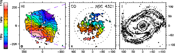
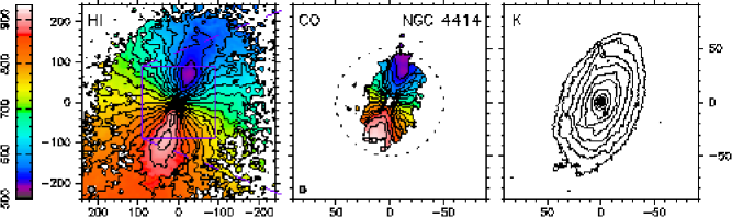
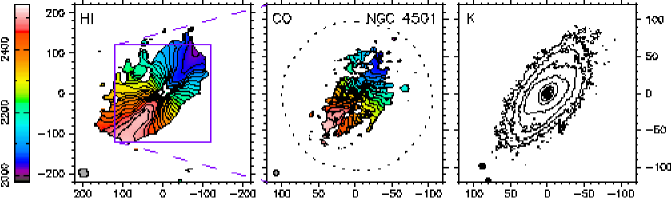
Figure 1.— Velocity fields for all seven galaxies derived from Gaussian fits as described in the text. For each galaxy, the left panel shows the H I velocity field, the center panel shows the full-resolution CO velocity field, and the right panel shows a contoured $I$ or $K$-band image (note the presence of some foreground stars). Units of the axes are in arcseconds. The velocity fields have been masked using a rotation model as described in the text. Isovelocity contours are spaced by 20 km s^-1. The synthesized beam is shown on the lower left, and the CO field of view (where the map sensitivity is at least half of its peak value) is given by a dotted contour.

3. Data Analysis

3.1. Velocity Fields

We derived CO and H I velocity fields from the corresponding datacubes by fitting a Gaussian to the spectrum at each pixel using a customized version of the MIRIAD task GAUFIT. Gaussian fits were required to have an amplitude of $>$1.5$\sigma$, where $\sigma$ is the r.m.s. noise in a channel map. Although this criterion allows for the detection of broad lines which are relatively weak in a single velocity channel, it has the drawback of also allowing for a large number of spurious fits, as evidenced by velocities which are spatially uncorrelated from pixel to pixel, producing a “noisy” appearance. In contrast, the true velocity field should be dominated by galactic rotation and smooth on scales smaller than a synthesized beam. Additional thresholds were therefore imposed based on the integrated flux of the Gaussian and the uncertainty in its mean velocity. Although the exact threshold depended somewhat on the signal-to-noise and flux level in the datacube, a Gaussian fit in a naturally weighted CO datacube ($\sigma\sim 50$ mJy bm^-1) would typically be required to have a velocity-integrated intensity of $\gtrsim 3$ Jy bm^-1 km s^-1 (a 3$\sigma$ detection over 20 km s^-1) and a velocity uncertainty of $\lesssim 20$ km s^-1 to be included. The assumption of Gaussian profiles, of course, is only an approximation, but in most cases the signal-to-noise could not justify the use of an asymmetric profile, and other methods of deriving the velocity field (such as the first moment) proved less robust and did not provide meaningful error estimates.

Figure 1 shows the CO and H I velocity fields at full resolution and a contoured $I$ or $K$-band image on the same scale as the CO velocity field for comparison. The BIMA field of view (where the sensitivity drops to half of its peak value) is shown as a dotted contour. The velocity fields shown have been masked further using a rotation model derived from the adopted rotation curve. This masking eliminates points which deviate by $\gtrsim$50 km s^-1 from circular rotation, as described in §3.2. As noted in Paper I, the CO emission in all galaxies except NGC 4736 and 5033 appears to extend to the edge of the observed field, suggesting that our observations sample only the inner part of the molecular disk.

Note that while there is some subjectivity in determining the appropriate thresholds for accepting the Gausssian fits, our velocity fields do not automatically reject anomalous velocity gas that is inconsistent with circular rotation, until the final masking using a rotation model is performed. Indeed an anomalous velocity component is seen in the southeastern corner of the H I disk in NGC 4501. No other clear examples of anomalous velocity gas were seen.

Table 3Galaxy Parameters From Kinematic Fits

Galaxy	$(\Delta x_{0},\Delta y_{0})$	$V_{\rm sys}$	$\Gamma_{0}$	$i$
	(″)	(km s-1)	(°)	(°)
NGC 4321	(0,0)	$1570\pm 3$	$153\pm 3$	$34\pm 5$
NGC 4414	(2,0)	$720\pm 5$	$159\pm 2$	$55\pm 2$
NGC 4501	(0,0)	$2270\pm 1$	$141\pm 1$	$64\pm 2$
NGC 4736	(1,1)	$317\pm 4$	$295\pm 10$	$32\pm 8$
NGC 5033	$(-1,0)$	$880\pm 8$	$353\pm 2$	$68\pm 2$
NGC 5055	(0,0)	$506\pm 3$	$98\pm 1$	$63\pm 1$
NGC 5457	(0,0)	$257\pm 1$	$42\pm 2$	$21\pm 3$

Figure 2.— A circular orbit in the plane of the galaxy as viewed from two different orientations: (a) oblique view, showing direction to the observer; and (b) observer’s view, with north up. The angles shown are as defined in the text.

3.2. Kinematic Disk Parameters

In preparation for the more detailed kinematic analysis needed to search for radial flows, we estimated the basic disk orientation parameters (mean velocity, rotation center, position angle, and inclination) as well as the rotation curve by fitting tilted-ring models to the CO and H I velocity fields. Four velocity fields were analyzed for each galaxy: the CO and H I at full resolution, the CO data smoothed to the resolution of the H I, and the H I data smoothed to 55″ resolution. We used the standard least-squares fitting technique developed by Begeman (1987), as implemented in the ROTCUR task within the NEMO software package (Teuben 1995). The galactic disk is subdivided into rings, each of which is described by 6 parameters: the center coordinates $(x_{0},y_{0})$, position angle ($\Gamma_{0}$), inclination ($i$), offset velocity ($V_{\rm sys}$), and circular velocity ($v_{c}$). Starting with initial estimates for the fitting parameters, the parameters are adjusted iteratively for each ring until convergence is achieved.

In general it is not possible to fit all 6 parameters simultaneously, due to kinematic disturbances and limited signal-to-noise in the velocity field, compounded by correlations between fit parameters. We therefore adopted the following procedure for determining the fit parameters:

1. Initial estimates for $i$ and $\Gamma_{0}$ were taken from the isophotal fits (§3.3), and the optical or radio continuum center from the NASA Extragalactic Database (NED) was taken as $(x_{0},y_{0})$. Initial estimates for $V_{\rm sys}$ and $v_{c}$ were taken from a position-velocity cut through the center at a position angle of $\Gamma_{0}$, or from previously published studies.

2. An improved estimate of $\Gamma_{0}$ was determined by fixing $(x_{0},y_{0})$, $V_{\rm sys}$, and $i$, and allowing the remaining parameters ($\Gamma_{0}$ and $v_{c}$) to vary.

3. An improved estimate of $V_{\rm sys}$ was determined by fixing $(x_{0},y_{0})$, $\Gamma_{0}$, and $i$.

4. An improved estimate of $(x_{0},y_{0})$ was determined by fixing $V_{\rm sys}$, $\Gamma_{0}$, and $i$.

5. An attempt was made to fit for $i$ while $(x_{0},y_{0})$, $V_{\rm sys}$, and $\Gamma_{0}$ were held fixed, although this could only be accomplished for some of the rings.

At each step, an inner radius for the fit was chosen to exclude rings within 2 beamwidths of the center, which were strongly affected by finite resolution effects (beam smearing). An outer radius was chosen to ensure that the ring was well-sampled in azimuth and did not show signs of a strong warp (a systematic drift in $\Gamma_{0}$ with radius). Since the program fits each ring separately, a weighted average of the values for all rings was used as the improved estimate for the next step. The full-resolution H I maps were generally most useful for constraining the fit parameters, since they contain a large number of independent resolution elements in a region where $v_{c}$ is roughly constant, but the CO maps provide better constraints on the kinematic center since they have higher resolution (and often signal-to-noise) in the central region.

Once an initial rotation curve and set of orientation parameters had been determined, model velocity fields were generated (assuming a flat rotation curve beyond the outer edge of the fitted disk) and compared to the observed velocity fields. Pixels in the velocity fields which were discrepant by more than $\sim$50 km s^-1 from the corresponding model were flagged. This threshold was increased when necessary so that only points that were clearly noise were rejected: care was taken to ensure that the threshold did not exclude gas that was continuous in velocity with gas in the disk. Although this process introduces some noise bias (noise pixels with velocities within 50 km s^-1 of the model are not eliminated), it provides an excellent compromise between sensitivity (which would be degraded by too strict a Gaussian fit threshold) and noise rejection, as evidenced by the generally smooth velocity contours in Fig. 1.

The cleaned velocity fields were then subjected to the ROTCUR analysis again to derive “final” values for the fit parameters, which are summarized in Table 3. The uncertainties given represent the range in values for the various velocity fields analyzed, and are thus generally larger than the formal least-squares errors for a single velocity field. In §4.5 we discuss how errors in the adopted disk parameters would affect the resulting harmonic decomposition.

Note that in most of the galaxies the kinematic center is displaced $<1\arcsec$ from the center defined by the $K$-band or radio continuum nucleus. Only NGC 4414 and 4736 show a displacement of $\sim$1$\farcs$5, which is of marginal significance given the uncertainties in determining the optical and kinematic centers. For the subsequent analyses presented here, we have adopted the kinematic rather than optical center.

3.3. Isophote Fits

In order to better constrain the influence of spiral structure and bars on the observed kinematics, we performed ellipse fitting to the optical and NIR isophotes using the IRAF task ELLIPSE. The fitting program outputs the center $(x,y)$ coordinates, semimajor axis $a$, ellipticity $\epsilon=1-b/a$, and position angle $\phi$ of each fit. The ellipse centers were fixed during the fitting except in the case of NGC 4321, for which a satisfactory fit could not be obtained without allowing the center to wander by up to $\sim$10″. However, the difficulty in fitting the isophotes does not reflect an uncertainty in the center position: the nucleus of NGC 4321 is well-determined photometrically in the $K$-band image (to within $\lesssim$2″) and the kinematic center is also well-determined (to within $\sim$1″) by the CO velocity field. The results of the isophotal analysis are discussed in §5.2.

4. Signatures of Non-Circular Motions in Disks

In this section we present some general results for non-circular motions in disks. We adopt a right-handed $xyz$ coordinate system with the main disk of the galaxy confined to the $xy$ plane. As discussed by Franx, van Gorkom, & de Zeeuw (1994), the direction of our sight-line is defined by two angles, $\theta_{\rm obs}$ and $i$, where $\theta_{\rm obs}$ is measured in the $xy$ plane from the $x$-axis and $i$ is measured from the $z$-axis [see Figure 2(a)]. Note that $i$ is restricted to the range $0<i<\pi/2$. Figure 2(b) then shows the appearance of the galaxy as viewed in the sky. Here $\Gamma$ is the position angle measured in the sky plane, from north to east, and $\Gamma_{\rm node}$ is the position angle of the line of nodes (the intersection of the galaxy and sky planes). Although in principle we could define the $x$-axis so that $\theta_{\rm obs}$=0, we choose to keep it independent of $\theta_{\rm obs}$ to more easily handle the case of a bar.

Adopting the convention that positive line-of-sight (“radial”) velocities correspond to recession, we therefore have:

$$V_{\rm los}=V_{\rm sys}+v_{c}\cos(\theta-\theta_{\rm obs}-\pi/2)\sin i$$ (1)

for an axisymmetric model with rotation curve $v_{c}(R)$. Here $V_{\rm sys}$ is the mean (systemic) velocity of the galaxy. For the most general case of a two-dimensional velocity field,

$$V_{\rm los}(x,y)=V_{\rm sys}+v_{\theta}(x,y)\cos\psi\sin i+v_{R}(x,y)\sin\psi\sin i\;,$$ (2)

where $(v_{R},v_{\theta})$ is the velocity vector in the disk in polar coordinates and $\psi\equiv\theta-\theta_{\rm obs}\mp\pi/2$ is the azimuthal angle in the galaxy plane, measured from the receding side of the line of nodes (the $-$ sign is taken for counterclockwise rotation and the $+$ sign for clockwise). With these definitions $v_{\theta}$ is always positive, and $v_{R}>0$ indicates outflow for counterclockwise rotation and inflow for clockwise rotation.

In each case below, we seek to express the model velocity field $V_{\rm los}$ in terms of harmonic coefficients $c_{j}(R)$ and $s_{j}(R)$, where

$$V_{\rm los}=c_{0}+\sum_{j=1}^{n}\left[c_{j}\cos(j\psi)+s_{j}\sin(j\psi)\right]$$ (3)

For the simple models we consider, it is only necessary to expand out to $n$=3. For the case of pure circular rotation, $c_{0}$=$V_{\rm sys}$ and $c_{1}$=$v_{c}\sin i$, with all other coefficients 0.

4.1. Axisymmetric Radial Flow

The simplest example of non-circular motion is one in which $v_{R}$ and $v_{\theta}$ are functions of radius $R$ only:

$$V_{\rm los}=V_{\rm sys}+v_{\theta}(R)\cos\psi\sin i+v_{R}(R)\sin\psi\sin i$$ (4)

This corresponds to circular motion superposed on axisymmetric inflow or outflow. The harmonic coefficients are simply $c_{0}$=$V_{\rm sys}$, $c_{1}$=$v_{\theta}\sin i$, and $s_{1}$=$v_{R}\sin i$. Of course, for the inflow case a continuity problem arises unless some sink for the inflowing gas exists: this might be star formation, a central black hole, or an outflowing wind ejected out of the plane.

4.2. Elliptical Streaming

A straightforward alternative to simple radial flows is the case in which gas follows elliptic closed orbits, as might occur in a bar-like potential. For a general distortion of harmonic number $m$ rotating at a fixed pattern speed $\Omega_{p}$, the potential is given by:

$$\Phi(R,\theta)=\Phi_{0}(R)+\Phi_{m}(R)\cos[m(\theta-\Omega_{p}t)]$$ (5)

where $\Phi_{0}$ is the axisymmetric part of the potential. For simplicity we take $\Phi_{0}$ to be a spherical logarithmic potential, giving a flat rotation curve with circular speed $v_{c}$:

$$\Phi_{0}(R)=v_{c}^{2}\ln R\;.$$

We assume a uniform $m$=2 perturbation to the potential given by:

$$\Phi_{2}=-\frac{1}{2}\epsilon_{\rm pot}v_{c}^{2}\;,$$

so that the ellipticity of the potential at all radii is $\epsilon_{\rm pot}$. The sign of $\Phi_{2}$ is taken to be negative in order that the equipotentials are elongated along the $x$-axis ($\theta$=0) at $t$=0. Potentials of this type have been analyzed in a number of previous studies (e.g., Franx et al. 1994; Kuijken & Tremaine 1994; Rix & Zaritsky 1995; Jog 2000).

Figure 3.— (a) Harmonic coefficients $s_{1}$ and $s_{3}$ normalized by $v_{*}=v_{c}\sin i$, plotted as a function of $\omega_{p}\propto R$ for a collisionless model (dashed line) and a dissipative model (solid line) with a flat rotation curve and a rotating, globally elongated potential. The locations of the ILR, CR, and OLR are marked as dotted lines. (b) Same but for a two-armed spiral model with a flat rotation curve, pitch angle of 10°, and velocity perturbation amplitude $v_{\rm sp}=0.2v_{c}$.

First we consider collisionless models, which are strictly applicable only to stellar orbits. Using the potential in Eq. 5 and the equation of motion in a frame rotating at angular velocity $\Omega_{p}$ (Binney & Tremaine 1987), one can solve for the allowed closed, periodic orbits using first-order epicyclic theory (this assumes the bar perturbation is relatively weak). Schoenmakers, Franx, & de Zeeuw (1997) showed that a potential distortion of order $m$ introduces changes in the $(m-1)$st and $(m+1)$st harmonic coefficients. For the $m$=2 case, their expressions reduce to:

$$c_{0} = V_{\rm sys}$$ (6)

$$c_{1} = v_{*}\left\{1-\frac{1}{4}[(2-3\omega_{p})a_{2}+(1-\omega_{p})b_{2}]\cos 2\theta_{\rm obs}\right\}$$

$$s_{1} = v_{*}\left\{\frac{1}{4}[(2-3\omega_{p})a_{2}+(1-\omega_{p})b_{2}]\sin 2\theta_{\rm obs}\right\}$$

$$c_{3} = v_{*}\left\{-\frac{1}{4}[(\omega_{p}-2)a_{2}+(1-\omega_{p})b_{2}]\cos 2\theta_{\rm obs}\right\}$$

$$s_{3} = v_{*}\left\{\frac{1}{4}[(\omega_{p}-2)a_{2}+(1-\omega_{p})b_{2}]\sin 2\theta_{\rm obs}\right\}$$

where $v_{*}\equiv v_{c}\sin i$, $\omega_{p}\equiv\Omega_{p}/\Omega_{0}=R(\Omega_{p}/v_{c})$, and the ellipticity coefficients $a_{2}$ and $b_{2}$ are given by:

$$a_{2} = \frac{1}{(1-4\omega_{p}+2\omega_{p}^{2})(1-\omega_{p})}\,\epsilon_{\rm pot}$$ (7)

$$b_{2} = \frac{2-3\omega_{p}+2\omega_{p}^{2}}{(1-4\omega_{p}+2\omega_{p}^{2})(1-\omega_{p})^{2}}\,\epsilon_{\rm pot}$$

The coefficients $s_{1}$ and $s_{3}$ for this model are plotted with a dashed line in Figure 3(a) as a function of $\omega_{p}$, which is proportional to the radius $R$. Note that between the ILR (inner Lindblad resonance, at $\omega_{p}=1-\sqrt{2}/2$) and OLR (outer Lindblad resonance, at $\omega_{p}=1+\sqrt{2}/2$), the $s_{1}$ and $s_{3}$ terms have opposite sign.

Although gas is not expected to follow collisionless orbits, Gerhard & Vietri (1986) and Franx et al. (1994) have argued that a collisionless treatment should be applicable to gaseous orbits if the potential is non-rotating, since gas will then be able to settle into stable closed orbits. The special case of a stationary potential ($\omega_{p}$=0) was solved previously by Franx et al. (1994):

$$c_{1} = v_{*}(1-\epsilon_{\rm pot}\cos 2\theta_{\rm obs})$$ (8)

$$s_{1} = v_{*}\epsilon_{\rm pot}\sin 2\theta_{\rm obs}$$

$$c_{3} = s_{3}=0$$

Here no resonances exist and all orbits are aligned along the $y$-axis, perpendicular to the bar. The fact that the $c_{3}$ and $s_{3}$ terms vanish has an important implication: for a flat rotation curve, the velocity field of a stationary bar potential resembles axisymmetric inflow or outflow. Thus kinematics alone cannot distinguish these two cases; in §4.6 we will discuss how photometric measurements might break this degeneracy. Since measurement of $c_{1}$ only provides the value of $v_{*}(1-\epsilon_{\rm pot}\cos 2\theta_{\rm obs})$, and $v_{*}$ cannot be determined independently, it is impossible to disentangle $\epsilon_{\rm pot}$ from the viewing angle $\theta_{\rm obs}$. However, under the assumption that $c_{1}\approx v_{*}$, a measurement of the $s_{1}$ term provides an estimate of the quantity $\epsilon_{\rm pot}\sin 2\theta_{\rm obs}$, and hence a lower limit on $\epsilon_{\rm pot}$.

For the more general case of gas flow in a rotating potential, as in a barred galaxy, it is possible to relax the collisionless assumption by including a damping term in the equation of motion to simulate the dissipative effect of gas viscosity. This can be done as described in Appendix A. The corresponding harmonic coefficients $s_{1}$ and $s_{3}$ are plotted with a solid line in Figure 3(a). Their behavior is qualitatively similar to the collisionless model, aside from a smoother variation near the resonances. For the non-rotating case, the dissipative and collisionless models yield the same coefficients.

To determine the effect of using a more realistic potential, we also ran models using the analytic potential employed by Wada (1994), which gives a rotation curve that can be parametrized as $v_{c}\propto R(R^{2}+a^{2})^{-3/4}$. Although the results differ in detail from the flat rotation curve case, the $s_{1}$ and $s_{3}$ coefficients still have opposite signs except near major resonances. The region where the rotation curve rises is associated with a second inner Lindblad resonance (the inner ILR) across which the coefficients both change sign.

4.3. Spiral Arm Streaming

A two-armed spiral density wave can be thought of as an $m$=2 perturbation with a phase shift that varies with radius. One would therefore expect that the velocity perturbations due to spiral arms would be in rough qualitative agreement with the results given in §4.2. For a more detailed analysis we adopt the linearized equations given by Canzian & Allen (1997) for the velocity perturbations due to a spiral potential, which are based on the original treatment given by Lin, Yuan, & Shu (1969). Substituting into their equations, we find for a two-armed logarithmic spiral the harmonic coefficients

$$\frac{c_{1}-v_{c}}{\sin i} = \frac{v_{\rm sp}}{2}\left(\frac{\kappa}{2\Omega}-\nu\right)\sin\left(2\theta_{\rm sp}-\chi\right)$$ (9)

$$\frac{s_{1}}{\sin i} = \frac{v_{\rm sp}}{2}\left(\frac{\kappa}{2\Omega}-\nu\right)\cos\left(2\theta_{\rm sp}-\chi\right)$$

$$\frac{c_{3}}{\sin i} = \frac{v_{\rm sp}}{2}\left(\frac{\kappa}{2\Omega}+\nu\right)\sin\left(2\theta_{\rm sp}+\chi\right)$$

$$\frac{s_{3}}{\sin i} = \frac{v_{\rm sp}}{2}\left(\frac{\kappa}{2\Omega}+\nu\right)\cos\left(2\theta_{\rm sp}+\chi\right)\;.$$

Here $\theta_{\rm sp}$ is the spiral phase, defined at a fiducial radius $R_{0}$ by

$$\theta_{\rm sp}=\frac{\ln(R/R_{0})}{\tan\chi}\;,$$

where $\chi$ is the pitch angle, the angle an arm makes with the tangent to a circle. The dimensionless frequency $\nu$ and epicyclic frequency $\kappa$ are defined as

$$\nu\equiv\frac{m(\Omega_{p}-\Omega)}{\kappa}\;,\quad\quad\kappa^{2}\equiv 4\Omega^{2}+R\frac{d\Omega^{2}}{dR}\;,$$

and $v_{\rm sp}$ is a velocity amplitude that depends on the strength of the spiral perturbation.

The $s_{1}$ and $s_{3}$ coefficients for a flat rotation curve are plotted in Figure 3(b) as a function of $\omega_{p}\propto R$. A characteristic of the spiral wave is the sinusoidal variation in the coefficients with radius—since the spiral has no preferred orientation, the observer in effect samples different orientations of the perturbed velocity field at different radii.

In a realistic treatment including the nonlinear effect of shocks, the spiral velocity perturbations will not be purely sinusoidal (e.g., Roberts & Stewart 1987), the peaks in Figure 3(b) will be narrower, and additional Fourier terms will occur. However, two basic properties of the model are worth noting since they are likely to be quite general. First, there is the change in dominance from the $s_{1}$ term to the $s_{3}$ term that occurs at corotation, which Canzian (1993) showed must occur when crossing a corotation resonance. The same phenomenon occurs in the bar model, although to a lesser degree [Figure 3(a)]. Second, the signs of $s_{1}$ and $s_{3}$ are the same near corotation (where $\nu=0$), but tend to take on opposite signs as one moves away from the corotation resonance (CR). For the bar models, on the other hand, the two coefficients have opposite signs at nearly all radii. As shown by Schoenmakers et al. (1997), this difference can be attributed to additional contributions to $s_{1}$ and $s_{3}$ that result from the radial variation in the phase of the potential.

4.4. Warped Disk

Although not directly related to radial gas flows, warps are a common feature in the outer H I disks of galaxies, and are well-known to have a significant effect on the observed velocity field (e.g., Bosma 1978). A warp is characterized by gas moving in circular orbits, but with the angular momentum vectors of the orbits not aligned as they would be in the case of a flat disk. Most galaxies are not strongly warped within their optical disks (for a review of observed properties of warps see Briggs 1990), so the plane of the inner disk defines a natural coordinate system for the galaxy.

The kinematics of warped galaxies can usually be well-modeled with a tilted-ring fit (Rogstad, Lockhart, & Wright 1974; Bosma 1981), in which the inclination $i$ and the major axis position angle $\Gamma_{\rm maj}$ are allowed to vary with radius. In contrast to the cases of radial flows or elliptical streaming, the kinematic axes $\Gamma_{\rm maj}$ and $\Gamma_{\rm min}$ (see §4.6) remain perpendicular, even as they drift with radius (Bosma 1981), since the gas flow is still circular. A harmonic decomposition of the velocity field using fixed disk parameters will display the characteristic signatures due to incorrect values of the position angle and inclination discussed below (§4.5). The coefficients $c_{1}$, $s_{1}$, $c_{3}$, and $s_{3}$ will all change with radius, with the $c_{1}$ and $s_{1}$ terms being most affected. Again this contrasts with the case of elliptical or spiral streaming, where changes in the $c_{3}$ and $s_{3}$ terms will dominate beyond the corotation radius.

4.5. Errors in the Parameters and Beam Smearing

We have assumed up to this point that the disk parameters used in making the harmonic expansion (namely, the kinematic center, inclination, and position angle) are correct. It is clear that this will not generally be the case, since the disk parameters will likely be derived from the velocity field under the assumption of circular rotation. Schoenmakers et al. (1997) analyzed the changes in the harmonic coefficients that result from using incorrect disk parameters, and found that the Fourier components due to non-circular motions will mix with those due to incorrect disk parameters. To first order, and assuming the errors in the position of the kinematic center are small compared to the radii of interest (satisfied for our galaxies, see Table 3), the following rules apply:

1. An error in the position angle $\Gamma_{0}$ leads to offsets in the $s_{1}$ and $s_{3}$ terms proportional to $v_{*}\equiv v_{c}\sin i$. The offset in $s_{1}$ is generally larger than that in $s_{3}$.

2. An error in the inclination $i$ leads to offsets in the $c_{1}$ and $c_{3}$ terms which are proportional to $v_{*}$. Because the $c_{1}$ term is large, the effect will only be detectable in the $c_{3}$ term.

3. An error in the kinematic center leads to offsets in the $c_{0}$, $c_{2}$, and $s_{2}$ terms proportional to $v_{*}/R$.

What is the effect of finite resolution (beam smearing) on the coefficients? Smoothing a datacube to lower resolution affects primarily the $c_{1}$ term (since the rotation curve rise becomes more gradual) and the $c_{3}$ term (since the isovels near the galaxy center become more parallel, leading to a lower fitted inclination). On the other hand, the $s_{1}$ and $s_{3}$ terms, which are sensitive to the kinematic position angle, should be relatively unaffected by beam smearing outside of the central few resolution elements, since smoothing an image should not lead to any net rotation of the velocity contours. (Of course, any small-scale variations in these terms will be smoothed out, but there should be no systematic offsets.) We have confirmed these effects using simulations of axisymmetric velocity fields convolved with both symmetric and asymmetric beams (for details see Wong 2000). We note, however, that our simulations have assumed an axisymmetric filled disk; if the gas distribution is very inhomogeneous, or confined to a small range in azimuth, it is conceivable that beam smearing could affect the measured $s_{1}$ and $s_{3}$ terms as well.

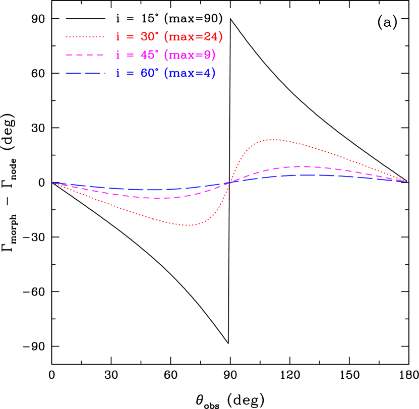
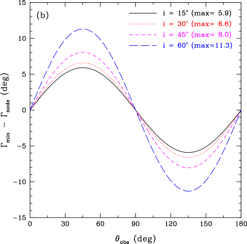
Figure 4.— (a) Offset of morphological position angle from the line of nodes, as a function of $\theta_{\rm obs}$, for isophotes of ellipticity 0.1. (b) Offset of kinematic minor axis position angle from the line of nodes, for an elongated potential with $\epsilon_{\rm pot}$=0.1. In both panels, a range of inclinations $i$ is shown. The numbers in parentheses in the legend give the maximum value (in degrees) for the corresponding curve.

4.6. Inclusion of Isophotal Data

Given that it is nearly impossible to kinematically distinguish a radial inflow model from an elliptical streaming model when $\omega_{p}\equiv\Omega_{p}/\Omega_{0}\ll 1$, i.e. when the potential is rotating slowly compared to the local circular speed, we must consider whether additional constraints can be provided by optical or near-infrared surface photometry. It is worth noting at the outset that since the isophotes (contours of constant surface brightness) of an axisymmetric disk are concentric aligned ellipses, any change in the isophotes over a region where the kinematics suggest pure radial flows would raise the possibility that streaming motions are occurring. A clearer prediction can only be made if one restricts consideration to an elliptical streaming model in which the gas orbits are elongated in the same direction as the isophotes. Then, as shown below, the morphological and kinematic position angles will deviate in opposite directions with respect to the line of nodes.

First, however, we need to identify conditions under which the elongation of the gas orbits will be parallel to the elongation of the isophotes. We consider three possibilities, two of which would satisfy this requirement:

1. For a stationary elongated potential, the closed loop orbits are perpendicular to the elongation of the potential, so if the stars follow loop-type orbits like the gas, the isophotes will be aligned with the gas orbits. In this case, however, the stars obviously cannot support the potential—in fact they will tend to counteract its asymmetry (Jog 2000). Rather, this case would be appropriate for a disk galaxy embedded in a massive triaxial halo.

2. Most of the stars could follow box-type orbits that are aligned with the potential, so that the isophotes are perpendicular to the gas orbits. This would allow a self-consistent solution between the stellar density and the potential it generates (de Zeeuw, Hunter, & Schwarzschild 1987), and no triaxial halo would be required.

3. The potential of a rotating bar will be aligned with the stable loop orbits between ILR and CR (these are often referred to as $x_{1}$ orbits), as shown in Figure 13 in the Appendix, so again the isophotes will be parallel to the gas orbits as in Case 1.

Thus, by assuming that the gas orbits are elongated parallel to the isophotes, we are assuming that Case 1 or 3 applies. Note that Case 1, which implies a strongly sub-maximal disk, conflicts with most observational studies of high surface brightness galaxies (Bell & de Jong 2001; Bottema 1993). On the other hand, Case 3 is not ruled out by such considerations and should be readily apparent in the isophotes, since bars are strong between the ILR and CR and weaker outside this region. We assume throughout our discussion that the isophotes trace a thin disk, so we can neglect the complications of projecting an inherently 3-dimensional structure onto the plane of the sky.

If an orbit (or isophote) has an intrinsic axis ratio $Q=b/a$ and position angle $\psi_{0}$ with respect to the line of nodes, how will it appear when projected on the sky at some inclination angle $i$? The appropriate geometrical transformations can be found in Teuben (1991), who finds that the new axis ratio $q$ and position angle $\gamma_{0}$ (still measured with respect to the line of nodes) are given by

$$q^{2}=\frac{(A\cos^{2}i+C)\cos 2\psi_{0}+(A\cos^{2}i-C)}{(A\cos^{2}i+C)\cos 2\psi_{0}-(A\cos^{2}i-C)}\\$$ (10)

$$\tan 2\gamma_{0}=-\frac{2B\cos i}{A\cos^{2}i-C}$$ (11)

where the coefficients are defined as

$$A \equiv Q^{2}\cos^{2}\psi_{0}+\frac{\sin^{2}\psi_{0}}{Q^{2}}$$ (12)

$$B \equiv \frac{(1-Q^{2})}{Q^{2}}\sin\psi_{0}\cos\psi_{0}$$

$$C \equiv Q^{2}\sin^{2}\psi_{0}+\frac{\cos^{2}\psi_{0}}{Q^{2}}\;.$$

Note that we have corrected some typesetting errors in the original paper by Teuben (1991).

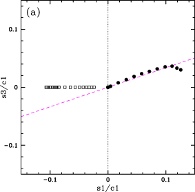
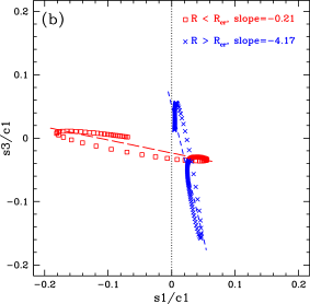
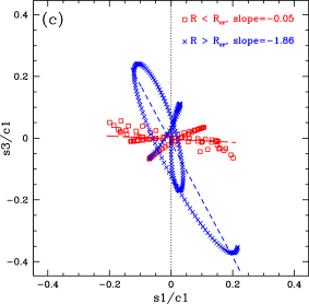
Figure 5.— Comparison of $s_{1}$ and $s_{3}$ coefficients for (a) inflow (open squares) and warp (solid circles) models, (b) bar streaming model including dissipation, and (c) spiral streaming model with a pitch angle of 10°. The dashed line in panel (a) represents the “warp line” where points should fall if there is an error in the P.A., for the assumed inclination of 55°. Long-dashed and short-dashed lines in panels (b) and (c) represent fits to points inside and outside of corotation respectively (shown with different plot symbols).

Using these equations and the sky coordinate system described by Figure 2, we can calculate the offset $\gamma_{0}$ between the apparent or morphological position angle of an elliptical isophote ($\Gamma_{\rm morph}$) and the position angle of the true line of nodes ($\Gamma_{\rm node}$). For the model discussed in §4.2, with equipotentials elongated along the $x$-axis, we assume that the isophotes are elongated along the $y$-axis. The resulting offset angle is shown in Figure 4(a) as a function of the viewing angle $\theta_{\rm obs}$ (measured from the $+x$-axis), for an ellipticity of 0.1 ($Q$=0.9) and a range of inclination angles. Note that for low inclinations ($\cos i>Q$), the offset angle can reach very large values if the line of sight is close to the long axis of the ellipse.

For comparison, the offset between the kinematic minor axis (the locus in the sky plane where $V_{\rm los}=V_{\rm sys}$) and the line of nodes, for an orbit in an elongated potential, is plotted in Figure 4(b) for the same set of inclination angles (the kinematic major axis shows a similar but weaker effect). This angle can be expressed in terms of the harmonic coefficients as (Franx et al. 1994):

$$\Gamma_{\rm min}-\Gamma_{\rm node}=\frac{\pi}{2}+\frac{s_{1}-s_{3}}{c_{1}-3c_{3}}\,\frac{1}{\cos i}\;.$$ (13)

For all non-degenerate observing angles, the offset in $\Gamma_{\rm min}$ is in the opposite direction from the offset in $\Gamma_{\rm morph}$. This is a robust result, depending purely on geometry, as can be seen by drawing on a sheet of paper an ellipse that is centered on, but has some angle to, the vertical and horizontal axes. The quadrants through which the apparent minor axis passes will be different from the quadrants where the maximum $y$-value is achieved, which is where the kinematic minor axis occurs if the $x$-axis is the line of nodes. Note also that a larger inclination reduces $\Gamma_{\rm morph}$ but increases $\Gamma_{\rm min}$, so bars in highly inclined galaxies are best identified kinematically rather than morphologically.

5. Results

Before returning to the analysis of the seven galaxies in our sample, let us summarize our basic approach to diagnosing various types of non-circular motions.

Based on the results of §4, the effects of elliptical or spiral streaming are most easily distinguished from radial inflow by examining the first and third order sine coefficients ($s_{1}$ and $s_{3}$). Variations in these coefficients as a function of radius can be placed into three broad categories, corresponding roughly to warp, elliptical streaming, and inflow models:

1. The $s_{1}$ and $s_{3}$ terms are correlated, with $ds_{3}/ds_{1}>0$.

2. The $s_{1}$ and $s_{3}$ terms are anti-correlated, with $ds_{3}/ds_{1}<0$.

3. The $s_{1}$ term is significant in some region but the $s_{3}$ term is negligible ($s_{3}\approx 0$).

We reiterate that these criteria do not always permit a clear distinction between physical models. As noted in §4.2, a stationary bar potential (usually in the second category) can mimic the kinematic signature of radial inflow (third category) inward of the ILR. A spiral streaming model (essentially equivalent to elliptical streaming, but with the orbits misaligned) can produce all three types of behavior, depending on location relative to the CR, but will generally correspond to case 2.

Examples of how four different kinematic models appear in the $s_{1}$-$s_{3}$ plane are given in Figure 5. For a pure warp model, the $(s_{1},s_{3})$ points are predicted to lie along a line we refer to as the “warp line,” defined by

$$\frac{\delta s_{1}}{\delta s_{3}}=\frac{3q^{2}+1}{1-q^{2}}\;,$$ (14)

where $q\equiv\cos i$. This is the predicted relation between $s_{1}$ and $s_{3}$ for an incorrect disk position angle (§4.5). For elliptical streaming, the results depend somewhat on the choice of model parameters, but in general one finds a shallow slope inside of the corotation radius ($R_{\rm CR}$) and a steep slope outside. This is a reflection of the switch in dominance from the $s_{1}$ to the $s_{3}$ term as one crosses $R_{\rm CR}$ (Canzian & Allen 1997), and also occurs for the spiral streaming model. As is clear from Figure 5, the greatest ambiguity arises when trying to distinguish inflow from streaming motions in the region $R\ll R_{\rm CR}$. For a large sample of galaxies viewed from random orientations, streaming motions should produce apparent outflow in roughly half of the galaxies, but our sample is too small for such statistical arguments to be useful.

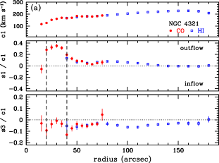
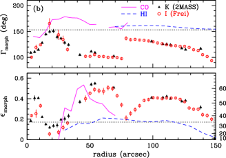
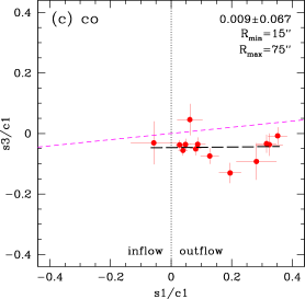
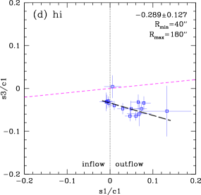
Figure 6.— (a) $c_{1}$, $s_{1}$ and $s_{3}$ coefficients plotted as functions of radius for NGC 4321. The $s_{1}$ and $s_{3}$ coefficients have been normalized by $c_{1}$. The CO data is indicated by filled circles and the H I data by open squares. Text labels indicate whether positive values of $s_{1}$ correspond to radial inflow or outflow. Vertical dashed lines delineate candidate inflow regions given in Table 4. (b) Morphological position angle and ellipticity as a function of radius from the isophote fits. In the upper panel, the kinematic minor axis position angle (shifted by $\pi/2$) is overplotted as a solid line for the CO and a dashed line for the HI, for all points with estimated error $<5\arcdeg$. In the lower panel, the kinematic inclination, expressed as an ellipticity using $\epsilon=1-\cos i$, is similarly plotted for points with error $<0.05$. Corresponding values of $i$ in degrees are given on the right axis. The dotted horizontal lines represent the adopted values for the disk position angle and inclination. (c) Comparison of $s_{1}$ and $s_{3}$ coefficients normalized by $c_{1}$, for CO and (d) HI. The heavy long-dashed line represents a linear least-squares fit to the data points (with slope given in the upper right corner), while the short-dashed line (“warp line”) represents the predicted relation between $s_{1}$ and $s_{3}$ for an error in the position angle $\Gamma_{0}$. The sign of $s_{1}$ corresponds to inflow or outflow as indicated at the bottom of each plot.

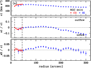
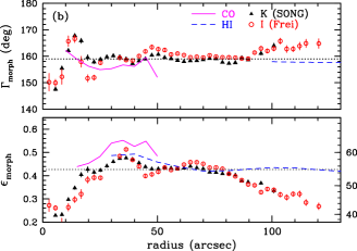
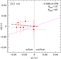
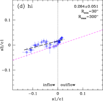
Figure 7.— Same as Fig. 6, but for NGC 4414.

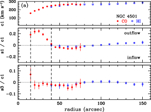
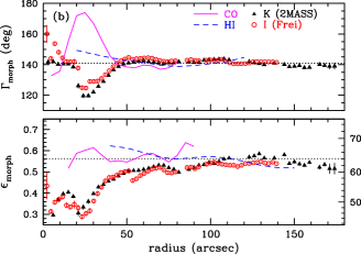
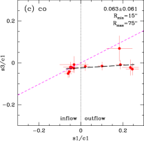
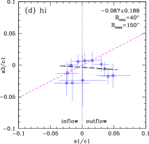
Figure 8.— Same as Fig. 6, but for NGC 4501.

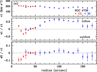
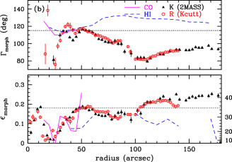
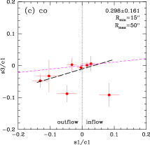
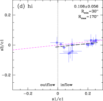
Figure 9.— Same as Fig. 6, but for NGC 4736.

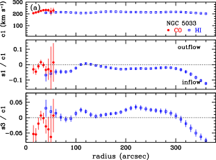
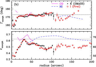
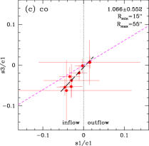
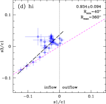
Figure 10.— Same as Fig. 6, but for NGC 5033.

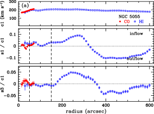
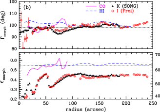
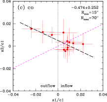
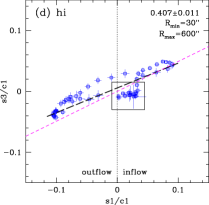
Figure 11.— Same as Fig. 6, but for NGC 5055. The box in panel (d) indicates the region of possible inflow between $R$=50″–150″.

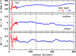
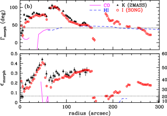
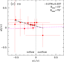
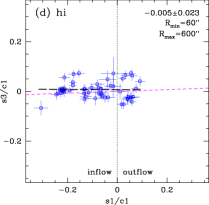
Figure 12.— Same as Fig. 6, but for NGC 5457.

5.1. Harmonic Analysis of Velocity Fields

Using the GIPSY task RESWRI (Schoenmakers 1999), each CO or H I velocity field was subdivided into rings using the adopted orientation parameters, and a third-order Fourier series was fitted to the velocities in each ring (cf. Eq. 3 with $n$=3). The program employs a least-squares fitting procedure (singular value decomposition) rather than a direct Fourier expansion since the points may not be uniformly distributed in azimuth. No extra weight is given to points near the major axis, and in fact it is points near the minor axis that provide the most information about non-circular motions.

The $s1$ and $s3$ coefficients are plotted against radius for each galaxy in Figures 6(a)–12(a), after normalization by $c_{1}\approx v_{*}$, which is also plotted. The error bars represent the formal least-squares errors (corrected for the number of pixels per beam), using the sum of fractional errors for the ratios. While the $c_{1}$ and $c_{3}$ terms are also affected by elliptical or spiral streaming, they are also quite susceptible to beam smearing effects and, in the case of the $c_{1}$ term, dominated by the overall circular rotation. Fluctuations in the $c_{0}$, $c_{2}$, and $s_{2}$ terms, on the other hand, reflect an error in the kinematic center (in which case the deviations should fall as $R^{-1}$) or the presence of an $m$=1 mode (lopsidedness) in the potential. Although lopsidedness is clearly revealed in several galaxies, it is usually at a fairly low level ($|c_{2}|\lesssim 5$ km s^-1), except in the outer H I disks of strongly warped galaxies. A more thorough analysis of this phenomenon is beyond the scope of this paper.

The lower panels of Figures 6–12 show, for each galaxy, the measured $s_{1}$ and $s_{3}$ terms plotted against each other, normalized by $c_{1}\approx v_{c}\sin i$. Coefficients for the CO and H I data are plotted separately as panels (c) and (d), since they are derived at different spatial resolutions. The slope of a linear least-squares fit (heavy long-dashed line) is given in the upper right corner of each plot; we consider slopes of $\lesssim 0.1$ in absolute value, corresponding to $|s_{1}/s_{3}|\gtrsim 10$, to be good candidates for radial flows. The dashed line through $(0,0)$ is the warp line—the locus of points along which an error in the disk position angle ($\Gamma$) should fall, assuming a flat rotation curve. A tendency for the data points fall close to this line would be consistent with a warp. In addition, a shift in the assumed P.A. ($\Gamma_{0}$) would be equivalent to a shift of all data points in a direction parallel to this line.

If the $s_{1}$ term is interpreted as radial flow, its sign corresponds to inflow or outflow depending on the sense of rotation in the galaxy. Assuming that spiral arms are always trailing, we infer that all galaxies besides NGC 4736 and 5055 rotate counterclockwise in the sky, so that except for these two galaxies the criterion $s_{1}>0$ corresponds to radial outflow, as labeled at the bottom of each $s_{1}$-$s_{3}$ plot. We discuss results for each galaxy individually in §5.3.

5.2. Comparison with Isophotal Data

Figures 6(b)–12(b) show, as functions of radius, the morphological position angle and inclination, as derived from the isophote fits, and the kinematic minor axis position angle and inclination, as derived from the harmonic decomposition of the CO and H I velocity fields. Horizontal dotted lines are used to indicate the adopted values of the position angle and inclination from the ROTCUR analysis (§3.2), except for NGC 4736 where the adopted inclination is based on the photometry of Möllenhoff, Matthias, & Gerhard (1995). The inclination $i$ has been expressed in terms of the ellipticity of the projected disk, $\epsilon\equiv 1-\cos i$. Note that the morphological inclination, $\epsilon_{\rm morph}$, is expected to decrease in the inner, bulge-dominated region of the disk as the isophotes become more circular. This general behavior is seen most clearly in NGC 4414, 4501, 5033, and 5055, which are sufficiently inclined so that the fitted values of $\Gamma_{\rm morph}$ and $\epsilon_{\rm morph}$ are dominated by geometry rather than non-axisymmetric structure.

The kinematic values were derived as follows:

1. We determined the kinematic minor axis $\Gamma_{\rm min}$ from the harmonic coefficients for each ring by setting $V_{\rm los}=V_{\rm sys}$ in Eq. 3 and deriving the roots numerically using Ridders’ method (Press et al. 1992, and references therein). There are two roots spaced by $\sim\pi$, corresponding to the two halves of the axis; we adopted the average of the two values (first offsetting one of them by $\pi$) and took half their difference as the estimated error $\sigma$. Only points with $\sigma<5\arcdeg$ are shown.

2. The kinematic inclination or “ellipticity” is defined by

   $$\epsilon_{\rm kin}=1-q_{\rm kin}=1-\widehat{q}\left(1-\frac{4c_{3}}{c_{1}}\right)$$ (15)

   where $\widehat{q}$ is the cosine of the adopted inclination used in the harmonic decomposition. This approximation is only accurate to first order in $\delta q/q$, and additional errors can arise if the rings are sufficiently tilted with respect to the assumed inclination that points in the velocity image get assigned to the wrong ring. We checked that our results were consistent with tilted-ring fits in which the inclination is allowed to vary, although such fits generally give poorer results because of correlations between fit parameters. Only points with $\sigma<0.05$ (with errors derived from the harmonic coefficients) are shown.

Based on the results of §4.6, we expect that elliptical streaming should be accompanied by a change in the morphological position angle $\Gamma_{\rm morph}$ in a direction opposite to the change in $\Gamma_{\rm min}$, assuming the gas orbits are aligned with the isophotes. An anti-correlation of this type is seen in several of the galaxies, most notably NGC 4321, 4501, and 4736, as discussed below. The presence of a bar, warp, or strong spiral structure would be expected to affect the morphological inclination (via the isophote ellipticity) and quite possibly the kinematic inclination (via the $c_{3}$ term) as well.

5.3. Results for Individual Galaxies

5.3.1 NGC 4321 (M100)

The CO velocity field of this well-studied Virgo cluster galaxy shows a strong $s_{1}$ term peaking between $R$=20″ and 40″ with $s_{1}/c_{1}\approx 0.35$ and a slope $|ds_{3}/ds_{1}|\approx-0.05$, making it a clear candidate for radial flows. Interpreted as radial flow, the $s_{1}$ term implies an outflow at $\sim$60 km s^-1 in the plane of the galaxy. However, elliptical streaming must be considered as well, since NGC 4321 is known to possess a stellar bar with a radial extent of $\sim$60″ (Knapen et al. 1995). Further evidence for elliptical streaming comes from a comparison of the kinematic and morphological position angles: the CO kinematics show a positive offset in $\Gamma_{\rm min}$ over the range $R$=20″–40″ [Fig. 6(b)], corresponding to a negative offset in $\Gamma_{\rm morph}$ over the same region. Moreover, the H I velocity field from $R$=40″–180″ shows a negative slope in the $s_{1}$-$s_{3}$ plane as expected for a bar potential [Fig. 6(d)]. The presence of a dominant $s_{1}$ term in the CO kinematics would be consistent with our modeling of gas flow in the ILR region of a barred galaxy [cf. Fig. 3(a)].

5.3.2 NGC 4414

The CO data show nearly circular kinematics, aside from a region near $R\sim 30\arcsec$ where $ds_{3}/ds_{1}\approx-0.1$ [Fig. 7(c)], a possible indication of radial inflow. The peak inflow speed would be $\sim$8 km s^-1, less than 4% of the circular speed. On the other hand, the errorbars are large and do not rule out values of $ds_{3}/ds_{1}$ that would be characteristic of an elliptical streaming model. While there is little evidence for a bar in the $K$-band image ($\Gamma_{\rm morph}$ varies by $<2\arcdeg$ over the region $R$=20″–50″), low-amplitude spiral structure had been noted in the $K$-band image by Thornley & Mundy (1997b) after removing an axisymmetric component from the light distribution. Thus the apparent inflow signature may be related to weak spiral streaming.

While the H I data show a strong decrease in the $s_{1}$ component, especially for $R>150\arcsec$, it is well correlated with changes in $s_{3}$ [Fig. 7(d)], suggesting the presence of a strong warp. The slope of the least-squares fit is a good match to the warp line, although there is a constant offset from that line which may indicate the effects of other non-circular motions. A decreasing trend in the morphological inclination supports an interpretation in which the warp extends as far in as $R\approx 30$″, well within the optical radius ($R_{25}\sim 100\arcsec$). This would explain the slight mismatch between the CO and H I rotation curves, since the average CO and H I inclinations would actually be different. We note, however, that effects other than a warp, such as finite thickness or flaring of the disk, might also affect the morphological inclination.

5.3.3 NGC 4501 (M88)

The CO data show an outflow signature very similar to that seen in NGC 4321, with implied outflow velocities of up to $\sim$45 km s^-1 in the region $R<40\arcsec$ [Fig. 8(a)]. As in the case of 4321, however, this could well be due to elliptical streaming, a possibility that is strongly favored by the remarkably clear anti-correlation between $\Gamma_{\rm min}$ and $\Gamma_{\rm morph}$ in this region. It is unclear whether such a signature could be attributed to spiral arms—strong spiral features are seen in both CO and H$\alpha$ maps (Paper I), but at an inclination of 64° the projection effects are severe. The $s_{1}$-$s_{3}$ plot for the H I data [Fig. 8(d)] shows a marginally negative slope at larger radii (with $s_{1}>0$, as would be the case for outflow), which is also likely to be a consequence of the bar. Note that although the isophotes in this outer region ($R$=50″–100″) are nearly circular, isophotes become less sensitive to non-axisymmetric structures as the disk inclination increases. We conclude that NGC 4501 is a likely example of a galaxy that is optically classified as unbarred but whose gas kinematics and inner near-infrared isophotes strongly suggest the presence of a bar.

5.3.4 NGC 4736 (M94)

This prototypical ringed galaxy contains a nuclear stellar bar and a corresponding CO bar (Wong & Blitz 2000). We attribute the large $s_{1}$ and $s_{3}$ terms in the CO data to the effects of the bar, although the scatter in the $s_{1}$-$s_{3}$ plot is large [Fig. 9(c)], partly due to the complicating effects of a strong spiral arc at $R\sim 25\arcsec$ whose streaming motions are distinct from the bar’s. The H I kinematics between $R$=50″ and 150″ show a strong $s_{1}$ term with $|ds_{3}/ds_{1}|\approx 0.2$. In an earlier paper (Wong & Blitz 2000), we had argued that the relative weakness of the $s_{3}$ term appeared to rule out an elliptical streaming model. The more sophisticated analysis presented in §4.2 suggests that instead we may be viewing elliptical streaming in the vicinity of an ILR; in fact, the prominent H$\alpha$ ring in this galaxy at $R=45\arcsec$ has been modeled as the ILR of a large-scale oval distortion (Gerin, Casoli, & Combes 1991). A pronounced decrease in $\Gamma_{\rm morph}$ occurs between $R$=50″–100″, also consistent with such a distortion [Fig. 9(b)]. While a warp model is not ruled out by the kinematics alone, due to the low inclination of the galaxy, the observed anti-correlation between $\Gamma_{\rm morph}$ and $\Gamma_{\rm min}$ would then be harder to account for.

5.3.5 NGC 5033

The CO data show some evidence for a warp based on the $s_{1}$-$s_{3}$ plot [Fig. 10(c)], although the uncertainties are large. No indication of radial inflow at speeds of $>$5% of the circular speed ($v_{c}\sim 200$ km s^-1) is seen for $R<55\arcsec$. For the H I data, the $s_{1}$ and $s_{3}$ terms are positively correlated at radii beyond 90″, raising the possibility that the galaxy’s warp, which only becomes prominent around $R_{25}$=320″, is pervasive throughout the galaxy, as suggested for NGC 4414. Such a disturbance may be related to the weak interaction of NGC 5033 with Holmberg VIII, as evidenced by the tidal H I plume on the southern side of the galaxy (Thean et al. 1997). However, the peak in $s_{1}$ and $s_{3}$ near $R$=110″ [Fig. 10(a)] might instead be the result of spiral streaming. The morphological inclination also falls with radius beyond $R$=30″–100″, although it does not closely follow the kinematic inclination [Fig. 10(b)]. It is possible that extinction or projection effects due to the galaxy’s high inclination may dominate over the warp, as far as the isophotes are concerned. A deeper $K$-band image would be useful for clarifying the situation.

5.3.6 NGC 5055

A strong negative slope in the $s_{1}$-$s_{3}$ plot for the CO data [Fig. 11(c)] suggests the presence of low-level streaming motions centered around $R$=30″. Although inspection of the $K$-band image does not reveal clear evidence of a bar, the isophotes do become “boxier” around this radius, leading to a dip in the ellipticity $\epsilon_{\rm morph}$. In spite of this localized deviation, the smallness of the $s_{1}$ term places an upper limit of $v_{R}\lesssim 5$ km s^-1 (3% of the circular speed) on the magnitude of any radial flows in the region $R$=15″–70″.

The H I kinematics are clearly dominated by a warp for $R>200\arcsec$ (0.5$R_{25}$). Inside of this radius, a possible region of gas inflow is seen, highlighted by the small box in Fig. 11(d). We interpret this weak feature (again amounting to radial motions of no more than 3% of the circular speed) to spiral streaming motions, since one finds CO and H I spiral arms crossing the galaxy’s minor axis at approximately these radii, where their effects are more likely to have an impact on the observed kinematics. Fluctuations in the isophotal parameters $\Gamma_{\rm morph}$ and $\epsilon_{\rm morph}$ are also apparent around $R\approx 70\arcsec$ [Fig. 11(b)], and are likely associated with spiral arms.

Note that for this galaxy, $\epsilon_{\rm morph}$ never rises to a value comparable to $\epsilon_{\rm kin}$. Aside from a few humps that may be attributed to spiral structure, the morphological inclination reaches a fairly constant value of around 57°, while the kinematics favor an inclination of 63°, also with very little scatter (this comparison is made well inside the region of the warp). One possibility is that the morphological inclination is reduced by the finite thickness of the stellar disk. A radius of 200″ corresponds to $\sim$10 kpc for this galaxy, so the projected minor axis at this radius should have a length of $\sim$4.5 kpc if the true inclination is 63°. If the minor axis is extended by 1 kpc due to a thick disk, however, the morphological inclination is reduced to 56°, consistent with the observed value.

5.3.7 NGC 5457 (M101)

The inclination of this galaxy is not well determined by either morphology or kinematics; the adopted value is based on fitting just two rings in the H I velocity field. However, our value of 21° is close to the 18° value of RC3 as well as the 22° that results from the Tully-Fisher relation of Pierce & Tully (1992) using an H I linewidth of 190 km s^-1.

Despite poor signal-to-noise in the inner arcminute, the CO velocity field shows strong evidence for large $s_{1}$ and $s_{3}$ terms [Fig. 12(c)], and indeed a substantial twist in the kinematic minor axis is seen in the tapered CO velocity field (Fig. 1). The slope of the $s_{1}$-$s_{3}$ relation appears to be negative and thus indicative of elliptical streaming. Identifying the bar in the optical images is difficult due to the strong spiral structure in this galaxy, but the bar-like CO and H$\alpha$ morphology, as well as the rise in the ellipticity of the isophotes across the region $R$=20″–60″ to a value much larger than in the rest of the disk, confirm the presence of a weak bar or oval distortion in the inner regions. The H I kinematics show a strongly decreasing $s_{1}$ term beyond $R$=200″ (0.2$R_{25}$) which is probably dominated by a large outer warp, with additional fluctuations in $s_{1}$ and $s_{3}$ at certain radii due to the strong spiral structure in this galaxy. Unfortunately, the inclination is too low to clearly distinguish the effects of the warp from possible radial flows.

Table 4Candidate Regions For Radial Flows, Based On $s_{1}/s_{3}$

Galaxy	Tracer	Radial Range	Maximum $v_{R}$	Interpretation
NGC 4321	CO	20″–40″	$56\pm 5$	Bar streaming
NGC 4414	CO	15″–45″	$-8\pm 2$	Spiral streaming
NGC 4501	CO	15″–40″	$48\pm 5$	Bar streaming
NGC 4501	HI	40″–150″	$10\pm 4$	Bar streaming
NGC 5055	H I	50″–150″	$-6\pm 1$	Spiral streaming
NGC 5457	H I	250″–600″	$-56\pm 5$	Outer warp

6. Discussion and Conclusions

We have carried out a search for radial flow signatures in the CO and H I velocity fields of seven nearby spirals by decomposing each elliptical ring into a third-order Fourier series. By requiring that $|s_{1}/s_{3}|\gtrsim 10$ over a significant range in radius, where $s_{1}$ amd $s_{3}$ are the coefficients of the $\sin\psi$ and $\sin 3\psi$ terms, we identified candidate regions for radial inflow or outflow as summarized in Table 4. Aside from NGC 5457, where an inflow signature is degenerate with a warp, we find photometric evidence for bars or spiral structure in all such regions, suggesting that elliptical streaming in a bar or spiral potential is the dominant contributor to non-circular motions. While inflow may be superposed on these motions, we find no unequivocal evidence for radial inflow alone. Three of the galaxies, NGC 4414, 5033 and 5055, show nearly pure circular rotation in their inner few kiloparsecs ($R\lesssim 60$″), with an upper limit to any radial inflows of $\sim$5–10 km s^-1, or 3–5% of the circular speed. These are probably the strictest limits that can be placed on radial gas flows in external galaxies.

Although our radial inflow limits are a small fraction of the circular speed, they cannot be used to rule out theoretical models that invoke radial flows, since such models generally predict even smaller inflow speeds. On the higher end of estimates is that by Blitz (1996), who estimates that an inflow velocity of $-7$ km s^-1 would be needed to completely replenish gas consumed by star formation in the inner Galaxy with H I from twice the solar radius. Given that estimates of the gas consumption time in our sample of galaxies are substantially longer than in the Milky Way (Paper I), such a high inflow rate would not be expected. Struck-Marcell (1991) discusses how radial flows can serve to maintain hydrodynamic stability in gaseous disks, but such flows are always subsonic ($\lesssim$5 km s^-1) and in fact reduce to zero for an $R^{-1}$ gas surface density profile. Struck & Smith (1999) further develop this idea into a steady-state model for a turblent multiphase ISM, predicting slow ($\sim$3 km s^-1) inflows of cold gas in the galaxy midplane. Pure chemical evolution models invoke even smaller inflow speeds (e.g. $\sim$1 km s^-1 in Portinari & Chiosi 2000) since they are concerned with steepening metallicity gradients in galaxies over timescales of many Gyr. Thus, our observations and analysis techniques have yet to reach the regime where such flows can be easily detected.

The results presented in this paper underscore the difficulty of detecting radial inflow in disks where a warp or $m$=2 distortion in the potential exists. Once such effects become dominant, they cannot be easily fitted and removed without performing a more sophisticated analysis than that performed here. For instance, by neglecting the important role of shocks in the gas component, we are unable to model the very processes (bars and spiral arms) that are most likely to lead to radial inflows in the inner regions of galaxies. Even with more sophisticated modeling, however, a leap in sensitivity and angular resolution will be needed to examine shock regions in detail. Similarly, our lack of knowledge about warps limits our ability to analyze the gas kinematics in the outskirts of galaxies. The default assumption, that warped orbits remain circular even as they move away from the principal plane, must be only a crude approximation. Since warps may be intimately related to infalling gas (Binney 1992), which in turn could induce radial flows, further modeling is clearly desirable.

An intriguing result from our analysis has been the possible detection of low-level kinematic warp signatures in NGC 4414 and 5033, at radii well inside the radius at which the warp becomes prominent (which is roughly the optical radius $R_{25}$). While spiral structure may confuse the picture in NGC 5033, it is unlikely to play a major role in NGC 4414, where the spiral structure is much more flocculent and the isophote fits seem to indicate an optical warp as well. The prominent kinematic warps in NGC 5055 and 5457 also appear well inside $R_{25}$, contrary to usual expectations (e.g., Briggs 1990). Since warps are often straightforward to identify in the $s_{1}$-$s_{3}$ plane, the harmonic decomposition technique will be valuable for assessing the radius at which warping begins, which in turn may shed light on the physical mechanisms that maintain warps.

Appendix A Effect of Dissipation on Gaseous Orbits

For a non-zero pattern speed, a collisionless weak bar model has the property that the stable periodic orbits change orientation (from parallel to perpendicular to the bar or vice versa) with each resonance crossing [Figure 13(a)]. Many of the resulting orbits intersect each other, and are hence not accessible to the gas component, since only one velocity is permitted for a fluid at a given spatial location. Instead, the gaseous orbits are expected to turn gradually between resonances, producing a spiral pattern [see Figure 13(b)]. Since cloud collisions, shocks, and energy dissipation lead to vastly more complex behavior than can be described by a model such as the one given in §4.2, this situation is generally examined with the help of numerical simulations, employing either a hydrodynamical or “sticky particle” approach.

One can obtain an approximate analytic description of gaseous orbits in a barred potential by introducing a damping term into the equations of motion, as has been done by various authors (e.g., Lindblad & Lindblad 1994; Wada 1994; Byrd et al. 1998). The additional term simulates a frictional force that is proportional to the velocity perturbation in the radial and/or azimuthal direction. For simplicity we consider damping in the radial direction only, following Wada (1994). (The more involved case of both radial and azimuthal damping is treated by Baker 2000). The first-order equation of motion (cf. Binney & Tremaine 1987, p. 148) is then:

$$\ddot{R_{1}}+2\Lambda\dot{R}_{1}+\kappa_{0}^{2}R_{1}=-\left[\frac{d\Phi_{m}}{dR}+\frac{2\Omega\Phi_{m}}{R(\Omega-\Omega_{p})}\right]_{R_{0}}\cos m\phi_{0}$$ (A1)

where $\Lambda$ is the damping term and $\phi_{0}\equiv(\Omega_{0}-\Omega_{p})t$. The solutions for $(R,\phi,v_{R},v_{\phi})$ in the rest frame of the bar are given by Sakamoto et al. (1999), although we have redefined some of the constants here to facilitate comparison with §4.2:

$$R = R_{0}\left[1-\frac{A}{2}\cos(2\phi_{0}+\delta_{0})\right]$$ (A2)

$$\phi = \phi_{0}+\frac{B}{4}\sin(2\phi_{0}+\beta_{0})$$ (A3)

$$v_{R} = v_{c}(1-\omega_{p})[A\,\sin(2\phi_{0}+\delta_{0})]$$ (A4)

$$v_{\phi} = v_{c}(1-\omega_{p})\left[1-\frac{A}{2}\cos(2\phi_{0}+\delta_{0})+\frac{B}{2}\cos(2\phi_{0}+\beta_{0})\right]$$ (A5)

The amplitudes of the epicyclic motion are given by

$$A = \frac{2}{R_{0}\sqrt{\Delta_{0}^{2}+16\Lambda^{2}(\Omega_{0}-\Omega_{p})^{2}}}\left[\frac{2\Phi_{2}(R_{0})}{R_{0}(1-\omega_{p})}+\Phi_{2}^{\prime}(R_{0})\right]$$ (A6)

$$B = \sqrt{(E+F)^{2}+2EF(\cos\delta_{0}-1)}$$ (A7)

where

$$E\equiv-\frac{2A}{1-\omega_{p}}\;,\quad F\equiv\frac{2\Phi_{2}(R_{0})}{v_{c}^{2}(1-\omega_{p})^{2}}\;.$$

The phase shifts of the orbit are given by

$$\tan\delta_{0}=-\frac{4\Lambda(\Omega_{0}-\Omega_{p})}{\Delta_{0}}\;,\quad\tan\beta_{0}=\frac{\sin\delta_{0}}{\cos\delta_{0}+(F/E)}\;.$$ (A8)

Note that in the limit that $\Lambda\rightarrow 0$, we have $A\rightarrow a_{2}$ and $B\rightarrow(a_{2}+b_{2})$, in terms of the coefficients of the collisionless model.

Transforming to the galaxy rest frame, we find that for $t=0$:

$$v_{R} = v_{c}\left[A(1-\omega_{p})\sin(2\theta+\delta_{0})\right]$$ (A9)

$$v_{\theta} = v_{c}\left[1-\frac{A}{2}\cos(2\theta+\delta_{0})+\frac{B}{2}(1-\omega_{p})\cos(2\theta+\beta_{0})\right]\;.$$ (A10)

Recall that the harmonic coefficients are defined by:

$$V_{\rm los} = V_{\rm sys}+(v_{\theta}\cos\psi+v_{R}\sin\psi)\sin i$$ (A11)

$$= c_{0}+c_{1}\cos\psi+s_{1}\sin\psi+c_{3}\cos 3\psi+s_{3}\sin 3\psi\;,$$

where $\psi=\theta-\theta_{\rm obs}-\pi/2$. Thus we find:

$$c_{0} = V_{\rm sys}$$ (A12)

$$\frac{c_{1}}{v_{*}} = 1-\frac{1}{4}[(-2\omega_{p}+1)A\cos(2\theta_{\rm obs}+\delta_{0})+(1-\omega_{p})B\cos(2\theta_{\rm obs}+\beta_{0})]$$

$$\frac{s_{1}}{v_{*}} = \frac{1}{4}[(-2\omega_{p}+1)A\sin(2\theta_{\rm obs}+\delta_{0})+(1-\omega_{p})B\sin(2\theta_{\rm obs}+\beta_{0})]$$

$$\frac{c_{3}}{v_{*}} = -\frac{1}{4}[(2\omega_{p}-3)A\cos(2\theta_{\rm obs}+\delta_{0})+(1-\omega_{p})B\cos(2\theta_{\rm obs}+\beta_{0})]$$

$$\frac{s_{3}}{v_{*}} = \frac{1}{4}[(2\omega_{p}-3)A\sin(2\theta_{\rm obs}+\delta_{0})+(1-\omega_{p})B\sin(2\theta_{\rm obs}+\beta_{0})]$$

where $v_{*}\equiv v_{c}\sin i$. These relations give the observed harmonic coefficients in terms of the orbit parameters $(A,B,\beta_{0},\delta_{0})$.

Figure 13.— Orbits viewed in the rotating frame for a (a) dissipationless bar model and (b) dissipative bar model with a flat rotation curve. The dashed lines at radii of $1-\sqrt{2}/2$, 1, and $1+\sqrt{2}/2$ are the ILR, CR, and OLR respectively.

For the case of an elongated potential discussed in §4.2, the orbit parameters ($A$, $B$, $\delta_{0}$, $\beta_{0}$) are given by:

$$A = -\frac{\epsilon_{\rm pot}}{(1-\omega_{p})\sqrt{(1-4\omega_{p}+2\omega_{p}^{2})^{2}+4\lambda^{2}(1-\omega_{p})^{2}}}$$ (A13)

$$B = -\sqrt{\left(\frac{2A}{1-\omega_{p}}+\frac{\epsilon_{\rm pot}}{(1-\omega_{p})^{2}}\right)^{2}+\frac{4A\epsilon_{\rm pot}}{(1-\omega_{p})^{3}}(\cos\delta_{0}-1)}$$ (A14)

$$\tan\delta_{0} = \frac{2\lambda(1-\omega_{p})}{1-4\omega_{p}+2\omega_{p}^{2}}$$ (A15)

$$\tan\beta_{0} = \frac{\sin\delta_{0}}{\cos\delta_{0}+\epsilon_{\rm pot}/[2A(1-\omega_{p})]}\;.$$ (A16)

where $\lambda\equiv\Lambda/\Omega_{0}$. With our choice of signs, $\delta_{0}\rightarrow-\pi$ at $\omega_{p}$=0 for $\lambda=0$. Model orbits calculated using these equations, using a flat rotation curve, are shown in Figure 13(b). Note that the damping term leads to a gradual change in orbit orientation near the ILR ($\omega_{p}=1-\sqrt{2}/2$), although the orbit oscillations still go nonlinear near the CR ($\omega_{p}=1$).

References

- Athanassoula (1992) Athanassoula, E. 1992, MNRAS, 259, 345
- Baker (2000) Baker, A. J. 2000, PhD thesis, California Institute of Technology
- Begeman (1987) Begeman, K. G. 1987, PhD thesis, Univ. of Groningen
- Bell & de Jong (2001) Bell, E. F. & de Jong, R. S. 2001, ApJ, 550, 212
- Binney (1992) Binney, J. 1992, ARA&A, 30, 51
- Binney & Tremaine (1987) Binney, J. & Tremaine, S. 1987, Galactic Dynamics (Princeton: Princeton U. Press)
- Blitz (1996) Blitz, L. 1996, in 25 Years of Millimeter Wave Spectroscopy, ed. W. B. Latter, S. J. E. Radford, P. R. Jewell, J. G. Mangum, & J. Bally (Dordrecht: Kluwer), 11
- Bosma (1978) Bosma, A. 1978, PhD thesis, Univ. of Groningen
- Bosma (1981) —. 1981, AJ, 86, 1825
- Bottema (1993) Bottema, R. 1993, A&A, 275, 16
- Braun (1995) Braun, R. 1995, A&AS, 114, 409
- Briggs (1990) Briggs, F. H. 1990, ApJ, 352, 15
- Byrd et al. (1998) Byrd, G. G., Ousley, D., & dalla Piazza, C. 1998, MNRAS, 298, 78
- Canzian (1993) Canzian, B. 1993, ApJ, 414, 487
- Canzian & Allen (1997) Canzian, B. & Allen, R. J. 1997, ApJ, 479, 723
- Chamcham & Tayler (1994) Chamcham, K. & Tayler, R. J. 1994, MNRAS, 266, 282
- Combes (1999) Combes, F. 1999, Ap&SS, 265, 417
- de Vaucouleurs et al. (1991) de Vaucouleurs, G., de Vaucouleurs, A., Corwin, H. G., Buta, R. J., Paturel, G., & Fouqué, P. 1991, Third Reference Catalogue of Bright Galaxies (New York: Springer-Verlag)
- de Zeeuw et al. (1987) de Zeeuw, P. T., Hunter, C., & Schwarzschild, M. 1987, ApJ, 317, 607
- Ferguson & Clarke (2001) Ferguson, A. M. N. & Clarke, C. J. 2001, MNRAS, 325, 781
- Ferrarese et al. (1996) Ferrarese, L. et al. 1996, ApJ, 464, 568
- Franx et al. (1994) Franx, M., van Gorkom, J. H., & de Zeeuw, T. 1994, ApJ, 436, 642
- Frei et al. (1996) Frei, Z., Guhathakurta, P., Gunn, J. E., & Tyson, J. A. 1996, AJ, 111, 174
- Gerhard & Vietri (1986) Gerhard, O. E. & Vietri, M. 1986, MNRAS, 223, 377
- Gerin et al. (1991) Gerin, M., Casoli, F., & Combes, F. 1991, A&A, 251, 32
- Helfer et al. (2003) Helfer, T. T., Thornley, M. D., Regan, M. W., Wong, T., Sheth, K., Vogel, S. N., Blitz, L., & Bock, D. C.-J. 2003, ApJS, 145, 259
- Ho et al. (1997) Ho, L. C., Filippenko, A. V., & Sargent, W. L. W. 1997, ApJS, 112, 315
- Jog (2000) Jog, C. J. 2000, ApJ, 542, 216
- Knapen et al. (1995) Knapen, J. H., Beckman, J. E., Heller, C. H., Shlosman, I., & de Jong, R. S. 1995, ApJ, 454, 623
- Knapen et al. (1993) Knapen, J. H., Cepa, J., Beckman, J. E., del Rio, M. S., & Pedlar, A. 1993, ApJ, 416, 563
- Kuijken & Tremaine (1994) Kuijken, K. & Tremaine, S. 1994, ApJ, 421, 178
- Lacey & Fall (1985) Lacey, C. G. & Fall, S. M. 1985, ApJ, 290, 154
- Lin et al. (1969) Lin, C. C., Yuan, C., & Shu, F. H. 1969, ApJ, 155, 721
- Lin & Pringle (1987) Lin, D. N. C. & Pringle, J. E. 1987, ApJ, 320, L87
- Lindblad & Lindblad (1994) Lindblad, P. O. & Lindblad, P. A. B. 1994, in Physics of the Gaseous and Stellar Disks of the Galaxy, ASP Conf. Series Vol. 66, ed. I. R. King (San Francisco: ASP), 29
- Martin & Kennicutt (2001) Martin, C. L. & Kennicutt, R. C. 2001, ApJ, 555, 301
- Merrifield (1992) Merrifield, M. 1992, AJ, 103, 1552
- Möllenhoff et al. (1995) Möllenhoff, C., Matthias, M., & Gerhard, O. E. 1995, A&A, 301, 359
- Norman et al. (1996) Norman, C. A., Sellwood, J. A., & Hasan, H. 1996, ApJ, 462, 114
- Pierce & Tully (1992) Pierce, M. J. & Tully, R. B. 1992, ApJ, 387, 47
- Portinari & Chiosi (2000) Portinari, L. & Chiosi, C. 2000, A&A, 355, 929
- Press et al. (1992) Press, W. H., Teukolsky, S. A., Vetterling, W. T., & Flannery, B. P. 1992, Numerical Recipes in FORTRAN, 2nd Ed. (Cambridge U. Press)
- Quillen et al. (1995) Quillen, A. C., Frogel, J. A., Kenney, J. D. P., Pogge, R. W., & DePoy, D. L. 1995, ApJ, 441, 549
- Regan et al. (2001) Regan, M. W., Thornley, M. D., Helfer, T. T., Sheth, K., Wong, T., Vogel, S. N., Blitz, L., & Bock, D. C.-J. 2001, ApJ, 561, 218
- Regan et al. (1997) Regan, M. W., Vogel, S. N., & Teuben, P. J. 1997, ApJ, 482, L143
- Rix & Zaritsky (1995) Rix, H. & Zaritsky, D. 1995, ApJ, 447, 82
- Roberts & Stewart (1987) Roberts, W. W. & Stewart, G. R. 1987, ApJ, 314, 10
- Rogstad et al. (1974) Rogstad, D. H., Lockhart, I. A., & Wright, M. C. H. 1974, ApJ, 193, 309
- Sackett (1997) Sackett, P. D. 1997, ApJ, 483, 103
- Sakamoto et al. (1999) Sakamoto, K., Okumura, S. K., Ishizuki, S., & Scoville, N. Z. 1999, ApJS, 124, 403
- Schoenmakers (1999) Schoenmakers, R. H. M. 1999, PhD thesis, Univ. of Groningen
- Schoenmakers et al. (1997) Schoenmakers, R. H. M., Franx, M., & de Zeeuw, P. T. 1997, MNRAS, 292, 349
- Shlosman et al. (1989) Shlosman, I., Frank, J., & Begelman, M. C. 1989, Nature, 338, 45
- Struck & Smith (1999) Struck, C. & Smith, D. C. 1999, ApJ, 527, 673
- Struck-Marcell (1991) Struck-Marcell, C. 1991, ApJ, 368, 348
- Teuben (1991) Teuben, P. 1991, in Warped Disks and Inclined Rings Around Galaxies, ed. S. Casertano, P. D. Sackett, & F. H. Briggs (Cambridge: Cambridge U. Press), 40
- Teuben (1995) Teuben, P. J. 1995, in Astronomical Data Analysis Software and Systems IV, ASP Conference Series Vol. 77, ed. R. A. Shaw, H. E. Payne, & J. J. E. Hayes (San Francisco: ASP), 398
- Thean et al. (1997) Thean, A. H. C., Mundell, C. G., Pedlar, A., & Nicholson, R. A. 1997, MNRAS, 290, 15
- Thornley (1996) Thornley, M. D. 1996, ApJ, 469, L45
- Thornley & Mundy (1997a) Thornley, M. D. & Mundy, L. G. 1997a, ApJ, 484, 202
- Thornley & Mundy (1997b) —. 1997b, ApJ, 490, 682
- Wada (1994) Wada, K. 1994, PASJ, 46, 165
- Wong (2000) Wong, T. 2000, PhD thesis, Univ. of California at Berkeley
- Wong & Blitz (2000) Wong, T. & Blitz, L. 2000, ApJ, 540, 771
- Wong & Blitz (2002) —. 2002, ApJ, 569, 157