TNG Near-IR Photometry of five Galactic Globular Clusters

We present near–infrared J and K observations of giant stars in five metal-poor Galactic Globular Clusters (namely M3, M5, M10, M13 and M92) obtained at the Telescopio Nazionale Galileo (TNG). This database has been used to determine the main photometric properties of the red giant branch (RGB) from the (K,J-K) and, once combined with the optical data, in the (K,V-K) Color Magnitude Diagrams. A set of photometric indices (the RGB colors at fixed magnitudes) and the major RGB evolutionary features (slope, bump, tip) have been measured. The results have been compared with the relations obtained by Ferraro et al. (2000) and with the theoretical expectations, showing a very good agreement.

1 Introduction

This paper is part of a long-term project devoted to the detailed study of the Red Giant Branch (RGB) properties of Galactic Globular clusters (GGCs) using the Color–Magnitude Diagrams (CMDs) and Luminosity Functions (LFs) in the near–infrared (IR) (see e.g. Ferraro et al. 2000, hereafter F00).

The near–IR spectral range is particularly suitable to study the cool stellar sequences, being the most sensitive to low temperatures. In addition, compared to the visual range, the reddening corrections and the background contamination by Main Sequence (MS) stars are much less severe, allowing to properly characterize the RGB even in the innermost core region of stellar clusters, affected by severe crowding. This is well known for two decades, and several authors have used IR photometry to derive the main RGB properties, starting from the pioneering survey of $\sim$30 GGCs by Frogel, Cohen & Persson (1983–hereafter FCP83), based on single–channel detectors and aperture photometry.

In the 90’s with the advent of bidimensional IR array detectors with pixel sizes and overall performances similar to those of optical CCDs, larger and more complete samples of Population II RGB stars with high photometric accuracy have been provided (see e.g. Davidge & Simons 1991, 1994a, 1994b; Ferraro et al. 1994; Minniti 1995; Minniti et al. 1995; Ferraro et al. 1995; Montegriffo et al. 1995; Kuchinski et al. 1995–hereafter K95; Kuchinski & Frogel 1995–hereafter KF95; Guarnieri et al. 1998; Ferraro et al. 2000; Momany et al. 2003).

By combining near–IR and optical photometry one can also calibrate a few major indices with a wide spectral baseline, which turn out to be very sensitive to the stellar parameters, like for example the (V-K) color index, possibly the best photometric thermometer for cool giants. F00 presented high-quality near-IR CMDs of 10 GGCs spanning a wide metallicity range which have been used $(i)$ to calibrate several observables describing the RGB physical and chemical properties; $(ii)$ to detect the major RGB evolutionary features as the RGB bump and the RGB tip; $(iii)$ to prepare followup observations devoted to better understand the mass loss process (see e.g. Origlia et al. 2002). In this paper we present an extension of the F00 work to five additional metal–poor GGCs.

The observations and data reduction are presented in §2, while §3 describes the properties of the observed CMDs. §4 is devoted to derive the mean RGB features from the combined study of CMDs and LFs. We summarize our conclusions in §5.

Figure 1: K,J-K (upper panels) and K,V-K (lower panels) CMDs for the observed clusters. The thick line in each panel indicates the fiducial ridge line of the RGB.

2 Observations and data reduction

A set of J and K images were secured at the Telescopio Nazionale Galileo (TNG), in the Canary Islands during 3 nights on May 10,11 and 13th, 2000, using the near-IR camera ARNICA equipped with a NICMOS-3 $256\times 256$ array detector. By using a magnification of 0.35 ${}^{\prime\prime}/px$, for a total field of view of $1.5^{\prime}\times 1.5^{\prime}$, 5 GGCs, namely M3, M5, M10, M13 and M92, have been observed. Table 1 lists the main parameters adopted for the program clusters: the metallicity in the original scale of Zinn (1985), in the Carretta & Gratton (1997) (hereafter CG97) scale, and the global scale as defined by Ferraro et al. (1999–hereafter F99), the reddening and the distance modulus from Table 1 of F99. The central region of the cluster was mapped in all the targets with the exception of M10 for which only a field at ${\sim}1$’ East from the cluster center was secured. In M92, besides the central field, an additional partially overlapping field has been observed at ${\sim}1.5$’ South–East from the cluster center.

During the observations the average seeing was $0.8^{\prime\prime}-1^{\prime\prime}$. Each acquired J and K image was the average of 120 single exposures of 1-s detector integration time (DIT). A series of typically 4 in J and 8–12 images in K were secured on each target, for a total integration time of ${\approx}$ 8 and 24 minutes in J and K, respectively. The sky was measured at a distance of ${\sim}$8’–10’ from the cluster center. More details on the pre–reduction procedure can be found in Ferraro et al. (1994), Montegriffo et al. (1995). For each field we combined all the available sky–corrected images, in order to obtain a median–averaged image with a signal to noise ratio ${\geq}50$.

The photometric reduction was carried out by using the ROMAFOT package (Buonanno et al. 1983; Buonanno & Iannicola 1989). The Point Spread Function (PSF) fitting procedure was adopted to determine the instrumental magnitude of the stars in the frame. The full description of the reduction procedure is shown in previous papers (see Ferraro et al. 1994, 1997) and it will not be repeated here. We just report that the automatic search for the object detection was performed (in each filter) in the median–averaged image. As usual, the mask with the object positions was used as input for the PSF–fitting procedure and a catalog listing the instrumental magnitudes measured in each image was obtained. Magnitudes in each filter were then transformed to a homogeneous photometric system. A final catalog with the average instrumental J and K magnitudes from different images of the same field was finally obtained.

Since the observations were performed under not perfect photometric conditions, we adopted the following procedure to calibrate the data–set:
i) The instrumental magnitudes were first transformed into the Two Micron All Sky Survey (2MASS) photometric system. Only zero–order polynomial transformations were used.

ii) The catalogs in the 2MASS photometric system were finally transformed into the F00 system by using the following transformations:

$J_{F00}=J_{2MASS}+0.06$

$K_{F00}=K_{2MASS}+0.05$

The transformations were empirically calibrated by using more then 5000 stars in common between the 2MASS catalogs and the catalogs presented by F00 for 10 GGCs.

Fig. 1 present the K,J-K CMDs for the observed clusters calibrated in the F00 system. An overall uncertainty of ${\pm}0.05$ mag in the zero point calibration, both in the J and K bands, has been estimated.

Table 1: Adopted parameters for the observed clusters.

Name	$[Fe/H]_{Z85}$	$[Fe/H]_{CG97}$	$[M/H]$	$E(B-V)$	$(m-M)_{0}$
M3	-1.66	-1.34	-1.16	0.01	15.03
M5	-1.40	-1.11	-0.90	0.03	14.37
M10	-1.60	-1.41	-1.25	0.28	13.38
M13	-1.65	-1.39	-1.18	0.02	14.43
M92	-2.24	-2.16	-1.95	0.02	14.78

Figure 2: Internal photometric errors for stars detected in the observed cluster sample. The rms values of the frame-to-frame scatter expressed in magnitudes are plotted as a function of the J (left panels) and K (right panels) calibrated magnitudes.

3 Color Magnitude Diagrams

More then 4500 stars are plotted in the (K,J–K) and (K,V–K) CMDs shown in Fig. 1. Since the IR observations mapped the central regions of the clusters, we mostly used optical photometry from HST (M3: Ferraro et al. (1997), Rood et al. (1999); M5: Sandquist et al. (1996); M13: Ferraro et al. (1997b); M92: Ferraro et al.(2003) in preparation).

The main features of the CMDs presented in Fig. 1 can be schematically summarized as follow:
i) The RGB is quite well populated and allows us a clean definition of the mean ridge line in all the program clusters. The observations reach $K{\approx}17$ mag and are deep enough to detect the base of the RGB at ${\Delta}K{\approx}7-8$ mag fainter than the RGB tip.
ii) In the combined CMDs the Horizontal Branch (HB) stars are clearly separable from the RGB stars. The HB appears as a sequence which has an almost vertical structure in all the CMDs. This is not surprising since intermediate metal–poor clusters are expected to have blue HB.
iii) The RGB is well populated in all program clusters, even in the brightest magnitude bin, with the possible exception of M10. The large size of the available sample allows a meanful estimate of the major evolutionary features along the RGB, namely the RGB bump and tip.

3.1 Internal Photometric errors

A reasonable estimate of the internal photometric accuracy of the IR photometry presented here can be estimated from the rms frame-to-frame scatter of multiple stars measurements. Fig. 2 shows the distribution of the obtained values (see Ferraro et al. 1991), for all the stars detected in each program cluster and in each band as a function of the final calibrated magnitude. As expected the internal errors significantly increase at fainter magnitudes due to photon statistics. In addition to this general trend, a number of stars show a ${\sigma}$ larger than the mean value: these stars are either variable stars (mainly RR Lyrae) observed at random phase (M 3, M 5 and M 92 harbor a large population of such variables) or stars lying in the innermost region of the clusters severely affected by crowding conditions. Nevertheless, over most of the RGB extension, the internal errors are quite low (${\sigma}_{K}{\sim}{\sigma}_{J}<0.03$ mag), increasing up to ${\sigma}_{K}{\sim}{\sigma}_{J}{\sim}0.06$ at $K{\geq}16$.

3.2 Comparison with previous photometry

The clusters presented here have been subject of several photometric and spectroscopic investigations in the optical, particularly M3 and M13, since they are a classical HB Second Parameter pair. However, only a few papers in the literature present IR photometry for these clusters.

Cohen, Frogel & Persson (1978) (hereafter CFP78) presented JHK aperture photometry for a selected sample of bright giants in the outer region of M3, M13 and M92. The advent of a modern generation of IR arrays has led to the study of the Turn Off (TO) region (see e.g. Davidge & Harris 1995a, b; Davidge & Courteau 1999; Lee et al. 2001, for M3, M13 and M92 respectively), or the MS (see e.g. Burckley & Longmore 1992, for M13). However, IR observations devoted to the study of the photometric properties of the RGB for the program clusters are still lacking and a systematic star to star comparison with the quoted photometric studies is not possible. As an example, Fig. 3 shows the comparison of our set with the few stars observed by CFP78, in the outer regions of M3, M13 and M92. For M3 the RGB mean ridge line by Lee et al. (2001) is also shown. As can be seen the agreement with CFP78 database is acceptable, only in M13 does our dataset appear systematically redder than the CFP78 data by ${\sim}0.03$. In M3 the agreement with the mean ridge line of Lee et al. (2001) is very good.

4 The main RGB features

In this section the main photometric indices and RGB features are derived and compared with those found by F00.

Figure 3: Comparison with previous photometry for three clusters: M3, M13 and M92. The bright giants by CFP78 are overplotted to our data as filled squares. The RGB mean ridge line by Lee et al. (2001) for M3 is also plotted.

4.1 The RGB fiducial ridge lines

Figure 4: RGB fiducial ridge lines for the observed GGCs (solid lines) in the $M_{K}$,(J-K)₀ (left panel) and M_K,(V-K)₀ (right panel) compared with those of F00 (dotted lines).

In order to obtain the RGB fiducial ridge lines for our cluster sample we followed the same strategy as in F00. First, we removed the HB stars from the CMDs and then we computed the fiducial ridge lines by using a low-order polynomial to fit the RGB stars, rejecting those at ${\geq}{\pm}2{\sigma}$ from the best-fit line.

The ridge lines obtained following this procedure are overplotted to the (K,J–K) and (K,V–K) CMDs shown in Fig. 1. In order to convert the RGB fiducial ridge lines into the absolute plane we adopted the distance scale defined in F99. The correction for reddening has been computed by using the reddening values listed in Table 1 (F99) and the extinction coefficient for the J and K bands, reported by Savage & Mathis (1979) $A_{J}/E(B-V)=0.87$ and $A_{K}/E(B-V)=0.38$ . The adopted values for the true distance modulus and reddening are listed in Table1.

Fig. 4 shows the observed RGB fiducial ridge lines in the absolute $M_{K}$,(J-K)₀ and $M_{K}$,(V-K)₀ planes for the observed clusters (heavy solid lines), the ridge lines of the 10 GGCs presented by F00 (dotted lines) are also plotted as reference. As expected, the mean ridge lines of the five intermediate–low metallicity clusters studied here lie in the bluer region of the diagrams.

4.2 The RGB location in Color and in Magnitude

Table 2: RGB $\rm(J-K)_{0}$ colors for the observed GCs at different magnitudes ($\rm M_{K}=-3,-4,-5,-5.5$).

Name	$[M/H]$	$(J-K)_{0}^{-5.5}$	$(J-K)_{0}^{-5}$	$(J-K)_{0}^{-4}$	$(J-K)_{0}^{-3}$
M3	-1.16	0.84${\pm}0.02$	0.79${\pm}0.02$	0.72${\pm}0.01$	0.66${\pm}0.01$
M5	-0.90	0.90${\pm}0.02$	0.86${\pm}0.02$	0.78${\pm}0.02$	0.71${\pm}0.01$
M10	-1.25	0.75${\pm}0.01$	0.72${\pm}0.01$	0.66${\pm}0.01$	0.60${\pm}0.01$
M13	-1.18	0.89${\pm}0.02$	0.85${\pm}0.02$	0.76${\pm}0.02$	0.69${\pm}0.01$
M92	-1.95	0.71 ${\pm}0.01$	0.68 ${\pm}0.01$	0.62${\pm}0.01$	0.57${\pm}0.01$

Table 3: RGB $\rm(V-K)_{0}$ colors for the observed GCs at different magnitudes ($\rm M_{K}=-3,-4,-5,-5.5$).

Name	$[M/H]$	$(V-K)_{0}^{-5.5}$	$(V-K)_{0}^{-5}$	$(V-K)_{0}^{-4}$	$(V-K)_{0}^{-3}$
M3	-1.16	3.33${\pm}0.09$	3.10${\pm}0.08$	2.73${\pm}0.06$	2.47${\pm}0.04$
M5	-0.90	3.38${\pm}0.09$	3.15${\pm}0.09$	2.76${\pm}0.07$	2.44${\pm}0.06$
M13	-1.18	3.16${\pm}0.09$	2.96${\pm}0.07$	2.62${\pm}0.05$	2.38${\pm}0.04$
M92	-1.95	2.95${\pm}0.07$	2.76${\pm}0.06$	2.50${\pm}0.05$	2.30${\pm}0.03$

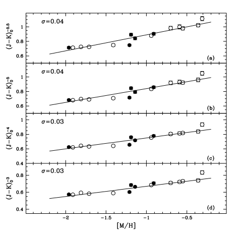
Figure 5: RGB mean (J-K)₀ color at different magnitudes ($\rm M_{K}=-3,-4,-5,-5.5$) as a function of the global metallicity for the observed clusters (filled circles). The data from F00 sample (empty circles) are also shown for comparison. The solid lines are the best-fit to the F00 data, while ${\sigma}$ is the standard deviation of the total sample (F00 and this work).

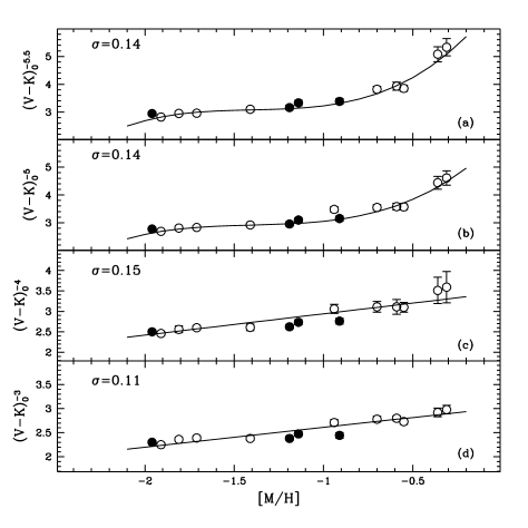
Figure 6: RGB mean (V-K)₀ color at different magnitudes ($\rm M_{K}=-3,-4,-5,-5.5$) as a function of the global metallicity for the observed clusters (filled circles) and for the F00 sample (empty circles). The solid lines are the best-fit to the F00 data, and ${\sigma}$ is the computed standard deviation of the total sample (F00 + this work).

In order to define the mean RGB properties of our cluster sample we used the observables defined in F00, namely: i) the intrinsic (J–K)₀ and (V–K)₀ colors at fixed absolute magnitude ${\rm(M_{K}=-3,-4,-5,-5.5)}$ and ii) the ${\rm M_{K}}$ absolute magnitude at constant color, both in the ${\rm M_{K}}$,(J–K)₀ and ${\rm M_{K}}$,(V–K)₀ planes. The intrinsic (J–K)₀ and (V–K)₀ colors of the RGB measured at different ${\rm M_{K}}$ are listed in Tables 2 and 3, respectively.

In order to perform a complete characterization of the RGB, these observables have been calibrated as a function of the cluster global metallicity ([M/H]) defined and computed in F99. As discussed in that paper the global metallicity take in account the contribution of the ${\alpha}$–elements in the definition of the total metallicity of the cluster.

Fig. 5 and 6 show the mean RGB (J–K)₀ and (V–K)₀ colors respectively, at different magnitude levels as a function of the global metallicity (filled circles). The value measured by F00 in the reference 10 GGCs are plotted as empty circles. The best fit to the F00 data is also shown in each panel. The five additional points, from this study, well fit into the F00 relations. Note that the Y-scale of panel (a) and (b) of Fig. 6 spans a much larger range in the V-K color than panel (c) and (d). This could produce the incorrect impression that the upper part of the RGB does not correlate with metallicity. Indeed, the linear region of the relations show in panel (a) and (b) have a slope (0.71 and 0.61, respectively) significantly larger than those shown in panel (c) and (d) (0.44 and 0.34, respectively). This evidence quantitatively confirms (according to Fig. 4) that the location in color of the upper part of the RGB is much more sensitive to the metallicity than the lower part.

Fig. 7 shows the trend of the $\rm M_{K}$ absolute magnitudes at fixed (V–K)₀=3 and (J–K)₀=0.7 colors as a function of the global metallicity, the solid lines being the best-fit to the F00 data. The derived values for $\rm M_{K}$ at different (V–K)₀ and (J–K)₀ are listed in Table 4. The values measured in our sample well fit into the relations calibrated by F00.

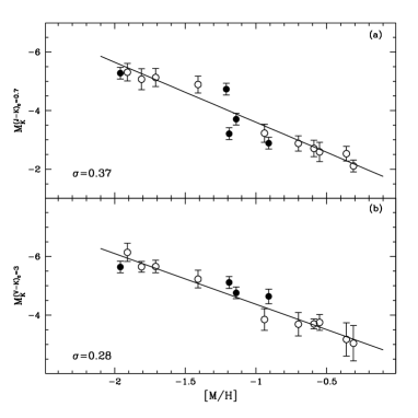
Figure 7: $M_{K}$ at constant (J-K)₀=0.7 (upper panel) and (V-K)₀=3 (lower panel) as a function of the global metallicity for the clusters in our sample (filled circles) and for the F00 sample (empty circles). The solid lines are the best-fit to the F00 data and ${\sigma}$ is the data standard deviation of the global sample (F00 and this work).

The errors on the derived absolute $\rm M_{K}$ have been computed by combining the two main sources of errors: the uncertainty in the absolute distance modulus (0.2 mag) and the uncertainty due to the reddening. In fact, given the intrinsic steepness of the RGB, an error of a few hundredths of magnitude in the reddening correction easily implies 0.15-0.20 mag uncertainty in the derived $M_{K}$ absolute magnitude, depending on the height along the RGB (see Fig. 4).

4.3 The RGB slope

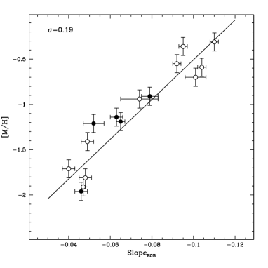
Figure 8: Global metallicity as a function of the derived RGB slope for the selected 5 GGCs (filled circles) and for the F00 sample (empty circles). The solid lines is the best-fit to the F00 data and ${\sigma}$ is the standard deviation of the global sample (F00 and this work).

One of the most useful parameters to derive the cluster metallicity is the slope of the brightest portion of the RGB (namely brighter than the HB), since it is a reddening and distance independent measurement. A careful estimate of the RGB slope is a complicated task, even in the K,J–K plane where the RGB morphology is less curved than in any other plane. However, adopting the technique described in K95 and KF95 we computed the RGB slope by means of a linear fit. The derived values are listed in Table 4, and Fig 8 shows the behaviour of this parameter as a function of the global metallicity. As usual, the analogous measurements and the average relation from F00 are plotted for comparison.

4.4 The RGB bump

Table 4: Calibrated RGB features for the observed clusters.

Name	$[M/H]$	$M_{K}^{(J-K)_{0}=0.7}$	$M_{K}^{(V-K)_{0}=3}$	SlopeRGB	$K^{Bump}$	$M_{K}^{Bump}$	$K^{Tip}$	$M_{K}^{Tip}$
M3	-1.16	-3.71${\pm}0.22$	-4.76${\pm}0.22$	-0.063${\pm}0.003$	13.15${\pm}0.05$	-1.88${\pm}0.21$	8.90${\pm}0.09$	-6.13${\pm}0.20$
M5	-0.90	-2.89${\pm}0.22$	-4.64${\pm}0.22$	-0.079${\pm}0.004$	12.70${\pm}0.06$	-1.68${\pm}0.24$	8.48${\pm}0.12$	-5.90${\pm}0.22$
M10	-1.25	-4.73${\pm}0.22$	——	-0.052${\pm}0.005$	——	——	——	——
M13	-1.18	-3.21${\pm}0.22$	-5.12${\pm}0.22$	-0.065${\pm}0.002$	12.45${\pm}0.05$	-1.99${\pm}0.21$	8.30${\pm}0.17$	-6.14${\pm}0.21$
M92	-1.95	-5.28${\pm}0.22$	-5.64${\pm}0.22$	-0.046${\pm}0.003$	12.40${\pm}0.05$	-2.39${\pm}0.21$	8.97${\pm}0.24$	-5.82${\pm}0.21$

Figure 9: Observed integrated (upper panel) and differential (lower panel) LF for M3. The dashed lines, in the upper panel, are the linear fits to the regions above and below the RGB bump.

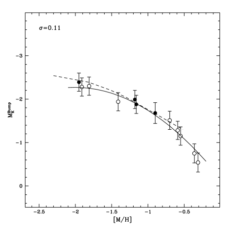
Figure 10: Absolute K magnitude at the RGB bump as a function of the global metallicity for our sample (filled circles) and for F00 dataset (empty circles). The solid line is the best fit to the F00 data. The dashed line is the theoretical prediction by Straniero et al. (1997).

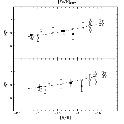
Figure 11: Absolute K magnitude of the brightest star (RGB tip) as a function of the metallicity in the CG97 (upper panel) and global scale (lower panel) for the GGCs in our sample (filled circles) and for F00 data–set (empty circles). The dashed lines are the theoretical expectations based on Straniero et al. (1997) models.

The RGB bump is an important evolutionary feature, since it flags the point (during the post–MS evolution of low mass stars) when the narrow hydrogen–burning shell reaches the discontinuity in the hydrogen distribution profile, generated by the previous innermost penetration of the convective envelope. Besides the obvious check of the accuracy of the theoretical models of stellar evolution, the identification of this feature in stellar aggregates can be used as a useful tool to provide observational constraints on a number of population parameters, since the RGB bump is a sensitive function of the metal content, helium abundance and the stellar population age. From an observational point of view, it was identified for the first time by King, Da Costa & Demarque (1985) in 47 Tuc. Then, during the last 10 years this feature was identified in a large number of GGCs (see e.g. Fusi Pecci et al. 1990; Zoccali et al. 2000, F99 and F00) and in other stellar aggregates (see e.g. Bellazzini et al. 2001, 2002; Monaco et al. 2002). As emphasized by Fusi Pecci et al. (1990) and by F99, the combined use of the differential and integrated LFs is the best tool in order to properly detect this feature. The bump luminosity increases with decreasing metallicity, hence its identification is more difficult in metal–poor clusters, where the brightest portion of the RGB is poorly populated because of the high evolutionary rate of stars at the end of the RGB evolution.

Following the Fusi Pecci et al. (1990) prescription, we identified the RGB bump in M3, M5, M13 and M92 by using the integral and differential LFs in the K band (as an example, both LFs are shown in Fig. 9 for M3). Since for M10 we did not map the central (more populated) regions of the cluster, the LF is much less populated than those observed in the other program clusters, preventing any reliable detection of the RGB bump. Note that the region covered by our observations allows to sample a significant fraction of the cluster light (ranging from 25% to 39% in 3 out of the 5 clusters presented here). However, in order to further increase the fraction of the sampled cluster population we also used complementary data from 2MASS catalog (after the application of the transformations quoted in §2). The level of the RGB-bump derived from our data was re-computed on the combined sample. Also, the RGB-bump magnitude in the K band was compared (by using the V-K color) with the RGB-bump in the V magnitude from F99 finding a very good agreement. The observed K^Bump and absolute M${}_{K}^{Bump}$ magnitude for the four clusters, where the bump has been identified, are listed in Table 4, while Fig. 10 shows the absolute K magnitude of the bump as a function of the global metallicity. The estimates for this additional sample of clusters well fit into the empirical relation by F00, with a total data standard deviation of ${\sigma}=0.11$. Fig. 10 also shows an excellent agreement with the theoretical expectations based on the Straniero et al. (1997) models (for an age of $t=14$ Gyr, see e.g. Gratton et al. 2003).

4.5 RGB Tip

The luminosity of the RGB tip (the bright end of the RGB) flags the end of the evolution along this sequence. The RGB tip luminosity is now recognized as a valuable standard candle (see e.g Bellazzini et al. 2001, and references therein) and it has been widely used to derive distance to extragalactic stellar populations (see e.g. Ferrarese et al. 2000a, b, and references therein). A well-defined relation between the bolometric luminosity of the brightest star and the cluster metallicity has been found by Frogel et al. (1981) and FCP83. F00 presented a more recent calibration of the RGB tip both in the K and bolometric magnitudes.

Here we present an estimate of the RGB tip for the program clusters by using the brightest giant in our observed sample (see F00). In principle, the magnitude of the brightest RGB star should give a reasonable estimate of the RGB tip if a significant fraction of the cluster has been sampled. Since we mapped, in most of the program clusters, the very central (more populated) regions we can reasonable apply this technique to our sample. The uncertainty of the procedure is discussed in F00, here we just note that the possible contamination of bright AGB stars is low since these stars are significantly less than the RGB stars, and especially in the intermediate–low metallicity clusters, no long-period AGB variables are expected. The main source of uncertainty is surely due to statistical fluctuations; following the prescription of F00 we estimated the error expected on the basis of the number of stars in the brightest two magnitude bin along the RGB. In our cluster sample ${\sigma}_{stat}$ turns to be ${\sim}$0.15 and we assume this as the main source of error in the RGB tip determination. The observed K magnitude of the brightest star and its absolute magnitude M_K are listed in columns 8 and 9, respectively, of Table 4. Fig. 11 shows the absolute K magnitude of the tip as a function of the metallicity in the CG97 and global scales, respectively. The theoretical expectation from Straniero et al. (1997) models for $t=14$ Gyr is also overplotted to the data. The data from F00 are also shown as empty circles. As can be seen from the figure, the theoretical prediction nicely agrees with the observations further suggesting that the adopted distance scale, from F99, is not affected by large systematic errors.

5 Conclusions

Using near-IR TNG observations of five low–metallicity GCCs, a detailed analysis of the RGB features has been performed. From the study of CMDs and LFs we derive and calibrate severals observables describing the morphology and the chemical properties of the RGB and the major RGB evolutionary features, namely

• the location in color and in magnitude of the RGB in the K,J–K and K,V–K planes

• the RGB slope

• the K–band absolute magnitude of the RGB bump and tip.

These observable have been also reported in the absolute planes by adopting the metallicity and distance scales defined in F99 and F00. The clusters presented in this paper represent an extension of the F00 sample, in the intermediate metal–poor regime. In a forthcoming paper an additional sample of intermediate–high metallicity clusters will be presented and updated relations for all the parameters will be derived and discussed.


We warmly thank Paolo Montegriffo for assistance during the catalog crosscorrelation procedure and the TNG staff for assistance during the observations. The financial support of the Agenzia Spaziale Italiana and the Ministero della Istruzione e della Ricerca Universitaria is kindly acknowledged.

This publication makes use of data products from the Two Micron All Sky Survey, which is a joint project of the University of Massachusetts and the Infrared Processing and Analysis Center/California Institute of Technology, founded by the National Aeronautics and Space Administration and the National Science Foundation.

References

- Arribas et al. (1990) Arribas, S., Martinez Roger, C., Paez, E. & Caputo, F. Ap&SS, 169, 45A
- Arribas et al. (1991) Arribas, S.,, Martinez Roger, C., Paez, E. & Caputo, F. A&AS, 88, 19A
- Bellazzini et al. (2001) Bellazzini, M., Ferraro, F. R. & Pancino, E. 2001, MNRAS, 327, 15
- Bellazzini et al. (2002) Bellazzini, M., Ferraro, F. R., Origlia, L., Pancino, E., Monaco, L. & Oliva, E. 2002, AJ, 124, 3222
- Buonanno et al. (1983) Buonanno, R., Buscema, G., Corsi, C. E., Ferraro, I. & Iannicola, G. 1983, A&A, 126,278
- Buonanno & Iannicola (1989) Buonanno, R. & Iannicola, G. 1988, PASP, 101, 294
- Burckley & Longmore (1992) Burckley, D. R. V. & Longmore, A. J. 1992, MNRAS, 257,731
- Carretta & Gratton (1997) Carretta, E. & Gratton, R. 1997, A&AS, 12, 95 (CG97)