The precession of orbital plane and the significant variabilities of binary pulsars

Abstract

There are two kinds of expressions on the precession of orbital plane of a binary pulsar system, which are given by Barker $\&$ O’Connell (1975) and Apostolatos et al. (1994), Kidder (1995) respectively. This paper points out that these two kinds of orbital precession velocities are actually obtained by the same Lagrangian under different degrees of freedom. Correspondingly the former expression is not consistent with the conservation of the total angular momentum vector; whereas the latter one is. Damour $\&$ Schäfer (1988) and Wex $\&$ Kopeikin (1999) have applied Barker $\&$ O’Connell’s orbital precession velocity in pulsar timing measurement. This paper applies Apostolatos et al. $\&$ Kidder’s orbital precession velocity in pulsar timing measurement. We analyze that Damour $\&$ Schäfer’s treatment corresponds to negligible Spin-Orbit induced precession of periastron. Whereas the effects corresponding to Wex $\&$ Kopeikin and this paper are both significant (however they are not equivalent). The observational data of two typical binary pulsars, PSR J2051-0827 and PSR J1713+0747 apparently support significant Spin-Orbit coupling effect. Further more, the discrepancies between Wex $\&$ Kopeikin and this paper can be tested on specific binary pulsars with orbital plane nearly edge on. If the orbital period derivative of double-pulsar system PSRs J0737-3039 A and B, with orbital inclination angle $i=87.7_{-29}^{+17}$deg, is much larger than that of the gravitational radiation induced one, then the expression of this paper is supported, otherwise Wex $\&$ Kopeikin’s expression is supported.

1 Introduction

In the gravitational two-body problem with spin, each body is precessing in the gravitational field of its companion, with precession velocity of 1 Post-Newtonian order (PN) (Barker $\&$ O’Connell 1975, hereafter BO). This precession velocity is widely accepted. But how the orbital plane reacts to the torque caused by the precession of the two bodies has two kinds of treatments. BO’s orbital precession velocity is obtained by assuming that the angular momentum vector, ${\bf L}$, precesses at the same velocity as the Runge-Lenz vector, ${\bf A}$.

On the other hand, in the study of the modulation of the gravitational wave by Spin-Orbit (S-L) coupling effect on merging binaries (Apostolatos et al. 1994, Kidder 1995, hereafter AK) obtain an orbital precession velocity that satisfies the conservation of the total angular momentum, ${\bf J}$, and the triangle constraint, ${\bf J}={\bf L}+{\bf S}$ (where ${\bf S}$ is the sum of spin angular momenta of two bodies, ${\bf S}_{1}$ and ${\bf S}_{2}$).

The discrepancy in the assumptions leads to different behaviors in physics between BO and AK’s orbital precession velocities. The former isn’t consistent with the triangle constraint, whereas the latter is. And the reason of this discrepancy is that the former actually assumes that the four vectors, ${\bf S}_{1}$, ${\bf S}_{2}$, ${\bf r}_{1}$ and ${\bf r}_{2}$ (${\bf r}_{1}$, ${\bf r}_{2}$ are position vectors of the two bodies respectively), are independent; whereas, the latter assumes that the independent vectors are either ${\bf S}_{1}$, ${\bf r}_{1}$ and ${\bf r}_{2}$; or ${\bf S}_{2}$, ${\bf r}_{1}$ and ${\bf r}_{2}$.

The discrepancy between BO and AK’s precession velocities is analogous to the following case. The motion of a small mass at the bottom of a clock pendulum can be described in $x-y$ plane. However if we treat the degree of freedom of this small mass as 2, then this small mass can move every in the 2-dimension space, and the length of the pendulum is not a constant. In other words, once the length of the pendulum is a constant, the degree of freedom is 1 instead of 2. Correspondingly if the free vectors of a binary system is 4, as treated by BO, then the triangle constraint cannot be satisfied (or ${\bf J}$ cannot be a constant vector). On the other hand, if the triangle constraint is satisfied, the number of free vectors is 3, instead of 4.

In the application to pulsar timing measurement, BO’s orbital precession velocity is treated in two different ways, by Damour $\&$ Schäfer (1988) and Wex $\&$ Kopeikin (1999) respectively. The former one predicts insignificant S-L coupling induced precession of periastron, $\dot{\omega}^{S}$, and the derivative of orbital period, $\dot{P}_{b}$; whereas the latter predicts significant $\dot{\omega}^{S}$ and $\dot{P}_{b}$. The paper points out that the discrepancy is due to Damour $\&$ Schäfer and Wex $\&$ Kopeikin calculated effects in different kinds of coordinate systems, the former coordinate system is not at rest to ”an observer” at the Solar System Baryon center (SSB), whereas, the latter is at rest to it. In other words, the former coordinate system has non-zero acceleration to SSB; whereas, the latter one has zero acceleration to SSB.

This paper calculates observational effect corresponding to AK’s orbital precession velocity, which uses the same coordinate system as that of Wex $\&$ Kopeikin (1999). Significant $\dot{\omega}^{S}$ and $\dot{P}_{b}$ are given, but they are not equivalent to the results given by Wex $\&$ Kopeikin (1999). The validity of these two expressions can be tested by specific binary pulsars with orbital inclination close to $\pi/2$, i.e., the double-pulsar system PSRs J0737-3039 A and B.

This paper contains four parts: (a) the physical discrepancy between BO and AK’s orbital precession velocity (Sect 2,3); (b) the derivation of S-L coupling induced effect corresponding to AK’s expression of orbital precession (Sect 4,5,9); (c) the discrepancy between the coordinate systems used by Damour $\&$ Schäfer (1988) and Wex $\&$ Kopeikin (1999), as well as the relationships among three kinds of S-L coupling induced effects, Damour $\&$ Schäfer and Wex $\&$ Kopeikin and this paper (Sect 6); (d) confrontation of the three S-L coupling effects with observational data of PSR J2051-0827 and PSR J1713+0747, and different predictions on $\dot{\omega}^{S}$ and $\dot{P}_{b}$ of PSRs J0737-3039 A and B by different S-L coupling models (Sect 7,8).

2 Orbital precession velocity

This section introduces the derivation of the orbital precession velocity of BO and AK.

2.1 Derivation of BO’s orbital precession velocity

BO’s two-body equation was the first gravitational two-body equation with spin, which consists of two parts, the precession velocity of the spin angular momenta vectors of body one and body two, and the precession velocity of the orbital angular momentum vector. Body one precesses in the gravitational field of body two, with precession velocity (BO),

$$\dot{\bf\Omega}_{1}=\frac{L(4+3m_{2}/m_{1})}{2r^{3}}\,\hat{\bf L}+\frac{S_{2}}{2r^{3}}\left[\hat{\bf S}_{2}-3(\hat{\bf L}\cdot\hat{\bf S}_{2})\,\hat{\bf L}\right]$$ (1)

where $\hat{\bf L}$, $\hat{\bf S}_{1}$ and $\hat{\bf S}_{2}$ are unit vectors of the orbital angular momentum, the spin angular momentum of star 1 and star 2, respectively.

$\dot{\bf\Omega}_{2}$ can be obtained by exchanging the subscript 1 and 2 at the right side of Eq.(1). The first term of Eq.(1) represents the geodetic (de Sitter) precession, which corresponds to the precession of ${\bf S}_{1}$ around ${\bf L}$, it is 1PN due to $\frac{L}{r^{3}}\sim(\frac{v}{c})^{2}(\frac{v}{r})$; and the second term represents the Lense-Thirring precession, ${\bf S}_{1}$ around ${\bf S}_{2}$, which is $\frac{S}{L}$ times smaller than the first, therefore, it corresponds to 1.5PN. The the precession velocity of the spin angular momenta vectors is confirmed by other authors using different method.

However for the precession velocity of the orbit, there are different expressions. BO’s orbital precession velocity is given as follows.

The total Hamiltonian for the gravitational two-body problem with spin is given (BO, Damour $\&$ Schäfer 1988),

$$H=H_{N}+H_{1PN}+H_{2PN}+H_{S}\ ,$$ (2)

where $H_{N}$, $H_{1PN}$ and $H_{2PN}$ are the Newtonian, the first and second order post-Newtonian terms respectively. $H_{S}$ is the spin-orbit interaction Hamiltonian (BO, Damour $\&$ Schäfer 1988),

$$H_{S}=\sum\limits_{\alpha=1}^{2}(2+3\frac{m_{\alpha+1}}{m_{\alpha}})(\frac{{\bf S}_{\alpha}\cdot{\bf L}}{r^{3}})\ ,$$ (3)

where $\alpha+1$ is meant modulo 2 (2+1=1), $m_{1}$, $m_{2}$ are the masses of the two stars, respectively, $r=a(1-e^{2})^{1/2}$, $a$ is the semi-major axis, $e$ is the eccentricity of the orbit. Notice we uses $G=c=1$ until discussing observational effects in Sec 5 to Sec 7.

The BO equation describes the secular effect of the orbital plane by a rotational velocity vector, $\dot{\Omega}_{S}$, acting on some instantaneous Newtonian ellipse. Damour $\&$ Schäfer (1988) computed $\dot{\Omega}_{S}$ in a simple manner by making full use of the Hamiltonian method. The functions of the canonically conjugate phase space variables ${\bf r}$ and ${\bf p}$ are defined as

$${\bf L}({\bf r},{\bf p})={\bf r}\times{\bf p}\ ,$$ (4)

$${\bf A}({\bf r},{\bf p})={\bf p}\times{\bf L}-GM\mu^{2}\frac{{\bf r}}{r}\ ,$$ (5)

where ${\bf r}={\bf r}_{1}-{\bf r}_{2}$, $M=m_{1}+m_{2}$, $\mu=m_{1}m_{2}/M$. The vector ${\bf A}$ is the Runge-Lenz vector (first discovered by Lagrange). The instantaneous Newtonian ellipse evolves according to the fundamental equations of Hamiltonian dynamics (Damour $\&$ Schäfer 1988)

$$\dot{\bf L}=\{{\bf L},H\}\ ,$$ (6)

$$\dot{\bf A}=\{{\bf A},H\}\ ,$$ (7)

where $\{,\}$ denote the Poisson bracket. ${\bf L}$ and ${\bf A}$ are first integrals of $H_{N}$, only $H_{1PN}+H_{2PN}+H_{S}$ contributes to the right-hand sides of Eq.(6) and Eq.(7), in which $H_{1PN}+H_{2PN}$ determines the precession of periastron, in 1PN it is given,

$$\dot{\omega}^{GR}=\frac{6\pi M}{P_{b}a(1-e^{2})}\ ,$$ (8)

where $P_{b}$ is the orbital period. To study the spin-orbit interaction, it is sufficient to consider $H_{S}$. Thus replacing $H$ of Eq.(6) and Eq.(7) by $H_{S}$ obtains (Damour $\&$ Schäfer 1988),

$$(\frac{d{\bf L}}{dt})_{S}=\{{\bf L},H_{S}\}=\dot{\Omega}_{S}^{\ast}\hat{{\bf S}}\times{\bf L}\ ,$$ (9)

$$(\frac{d{\bf A}}{dt})_{S}=\{{\bf A},H_{S}\}=\dot{\Omega}_{S}^{\ast}[\hat{{\bf S}}-3(\hat{{\bf L}}\cdot\hat{{\bf S}})\hat{{\bf L}}]\times{\bf A}\ .$$ (10)

where

$$\dot{\Omega}_{S}^{\ast}=\frac{S(4+3m_{2}/m_{1})}{2r^{3}}\ .$$ (11)

By Damour $\&$ Schäfer (1988), ${\bf S}$ represents a linear combination of ${\bf S}_{1}$ and ${\bf S}_{2}$. For simplicity of discussion, and for consistence with Wex $\&$ Kopeikin’s application of $\dot{\bf\Omega}_{S}$ (Wex $\&$ Kopeikin 1999), we assume ${\bf S}={\bf S}_{1}$ (the other spin angular momentum is ignored) until Sec 4 where the general binary pulsar is discussed.

The solution of Eq.(9) and Eq.(10) gives the S-L coupling induced orbital precession velocity (Damour $\&$ Schäfer 1988)

$$\dot{\bf\Omega}_{S}=\dot{\Omega}_{S}^{\ast}[\hat{{\bf S}}-3(\hat{{\bf L}}\cdot\hat{{\bf S}})\hat{{\bf L}}]\,.$$ (12)

By Eq.(9) and Eq.(12), the first derivative of $\hat{\bf L}$ can be obtained,

$$\frac{d\hat{\bf L}}{dt}=\dot{\Omega}^{\ast}_{S}\hat{\bf S}\times\hat{\bf L}\ ,$$ (13)

and by Eq.(1) the first derivative of $\hat{\bf S}$ (recall ${\bf S}={\bf S}_{1}$) can be written

$$\frac{d\hat{\bf S}}{dt}=\dot{\Omega}^{\ast}_{1}\hat{\bf L}\times\hat{\bf S}=\Omega^{\ast}_{S}\frac{L}{S}\hat{\bf L}\times\hat{\bf S}\ ,$$ (14)

where $\dot{\Omega}^{\ast}_{1}$ is the first term at the right hand side of Eq.(1). By Eq.(13) and Eq.(14) $\hat{\bf L}$ precesses slowly around $\hat{\bf S}$, 1.5PN, as shown by Eq.(13); whereas $\hat{\bf S}$ precesses rapidly around $\hat{\bf L}$, 1PN, as shown in Eq.(14). Therefore the BO equation predicts such a scenario that the two vectors, $\hat{\bf L}$ and $\hat{\bf S}$ precess around each with very different precession velocities (typically one is larger than the other by 3 to 4 orders of magnitude for a general binary pulsar system).

2.2 Orbital precession velocity in the calculation of gravitational waves

In the study of the modulation of precession of orbital plane to gravitational waves, the orbital precession velocity is obtained in a different manner and the result is very different from that given by Eq.(12).

Since the gravitational wave corresponding to 2.5PN, which is negligible compared with S-L coupling effect that corresponds to 1PN and 1.5PN, the total angular momentum can be treated as conserved, $\dot{{\bf J}}=0$. Then the following equation can be obtained (BO),

$$\dot{\bf\Omega}_{0}\times{\bf L}=-\dot{\bf\Omega}_{1}\times{\bf S}_{1}-\dot{\bf\Omega}_{2}\times{\bf S}_{2}\ \,.$$ (15)

Notice that as defined by BO and AK, ${\bf L}=\mu M^{1/2}r^{1/2}\hat{\bf L}$. In the one-spin case the right hand side of Eq.(15) can be given (Kidder 1995),

$$\dot{\bf S}=\frac{1}{2r^{3}}(4+\frac{3m_{2}}{m_{1}})({\bf L}\times{\bf S})\,,$$ (16)

and considering that ${\bf J}={\bf L}+{\bf S}$, Eq.(16) can be written,

$$\dot{\bf S}=\frac{1}{2r^{3}}(4+\frac{3m_{2}}{m_{1}})({\bf J}\times{\bf S})\ \,.$$ (17)

From Eq.(15), $\dot{\bf L}$ can be given,

$$\dot{\bf L}=\frac{1}{2r^{3}}(4+\frac{3m_{2}}{m_{1}})({\bf J}\times{\bf L})\ \,.$$ (18)

By Eq.(17) and Eq.(18), ${\bf L}$ and ${\bf S}$ precess about the fixed vector ${\bf J}$ at the same rate with a precession frequency approximately (AK)

$$\dot{\bf\Omega}_{0}=\frac{{\bf J}}{2r^{3}}(4+\frac{3m_{2}}{m_{1}})\ .$$ (19)

Eq.(19) indicates that in the 1 PN approximation, $\hat{\bf L}$ and $\hat{\bf S}$ can precess around ${\bf J}$ rapidly (1PN) with exactly the same velocity. Notice that the misalignment angles between $\hat{\bf L}$ and $\hat{\bf S}$ ($\lambda_{LS}$), $\hat{\bf L}$ and $\hat{\bf J}$ ($\lambda_{LJ}$) are very different, due to $S/L\ll 1$ , $\lambda_{LJ}$ is much smaller than $\lambda_{LS}$.

Thus, AK’s equations, Eq.(18) and Eq.(17), correspond to a very different scenario of motion of ${\bf S}$, ${\bf L}$ and ${\bf J}$ from that given by BO equation shown in Eq.(13) and Eq.(14).

3 Physical differences between BO and AK

This section compares two different scenarios corresponding to BO and AK’s orbital precession velocity, and points out that BO’s orbital precession velocity is actually inconsistent with the definition of the total angular momentum of a binary system.

Section 2 indicates that BO and AK derived the orbital precession velocity in different ways, therefore two different orbital precession velocity vectors are obtained, as shown in Eq.(12) and Eq.(19), respectively, which in turn correspond to different scenarios of motion of the three vectors. This section analyzes that the discrepancy between BO and AK is not just a discrepancy corresponding to different coordinate systems. Actually there is significant physical differences between BO and AK. The total angular momentum of a binary system is defined as BO

$${\bf J}={\bf L}+{\bf S}\ ,$$ (20)

Eq.(20) means that ${\bf J}$, ${\bf L}$ and ${\bf S}$ form a triangle, and therefore, it guarantees that the three vectors must be in one plane at any moment. For a general radio binary pulsar system, the total angular momentum of this system is conserved in 1PN. Therefore we have

$$\dot{\bf J}=0\ .$$ (21)

Eq.(21) means that ${\bf J}$ is a constant during the motion of a binary system. Eq.(21) and Eq.(20) together provide a scenario that the triangle formed by ${\bf L}$, ${\bf S}$ and ${\bf J}$ determines a plane, and the plane rotates around a fixed axis, ${\bf J}$, with velocity $\dot{\Omega}_{0}$. This scenario is shown in Fig 1. which can also be represented as

$$\dot{\bf J}=\dot{\Omega}_{0}\hat{\bf J}\times{\bf L}+\dot{\Omega}_{0}\hat{\bf J}\times{\bf S}=0\,,$$ (22)

Smarr $\&$ Blandford (1976) mentioned the scenario that ${\bf L}$ and ${\bf S}$ must be at opposite side of ${\bf J}$ at any instant. Hamilton and Sarazin (1982) also study the scenario and state that ${\bf L}$ precesses rapidly around ${\bf J}$. Obviously the orbital precession velocity given by Eq.(19) can satisfy the two constraints, Eq.(20) and Eq.(21) simultaneously.

Can the BO’s orbital precession velocity given by Eq.(12) satisfy the two constraints, Eq.(20) and Eq.(21) simultaneously ? From Eq.(12), Eq.(13) and Eq.(14), the first derivative of ${\bf J}$ can be written (BO)

$$\dot{\bf J}=\dot{\bf\Omega}_{S}\times{\bf L}+\dot{\bf\Omega}^{\ast}_{1}\times{\bf S}=\dot{\Omega}^{\ast}_{S}\hat{\bf S}\times{\bf L}+\dot{\Omega}^{\ast}_{1}\hat{\bf L}\times{\bf S}\equiv 0\ ,$$ (23)

and since Eq.(20) is defined in BO’s equation, then it seems that the BO equation can satisfy both Eq.(20) and Eq.(21).

But in BO’s derivation of $\dot{\bf\Omega}_{S}$ (Eq.(6)–Eq.(12)), Eq.(20) is never used. The corresponding $\dot{\bf\Omega}_{S}$ can make $\dot{\bf J}=\dot{\bf L}+\dot{\bf S}\equiv 0$, as shown in Eq.(23), however it cannot guarantee that ${\bf J}={\bf L}+{\bf S}$ is satisfied. In other words, when ${\bf J}\neq{\bf L}+{\bf S}$, Eq.(23) is still correct. This can be easily tested by putting ${\bf L}^{\prime}={\bf L}+\alpha{\bf S}$, or ${\bf S}^{\prime}={\bf S}+\beta{\bf L}$ ($\alpha$ and $\beta$ are arbitrary constants) into Eq.(23) to replace ${\bf L}$ and ${\bf S}$, respectively, obviously in such cases, Eq.(23) is still satisfied ($\dot{\bf J}\equiv 0$).

Contrarily in AK’s derivation of $\dot{\bf\Omega}_{0}$(Eq.(16)–Eq.(18)), the relation Eq.(20) is used. And if we do the same replacement of ${\bf L}^{\prime}={\bf L}+\alpha{\bf S}$, or ${\bf S}^{\prime}={\bf S}+\beta{\bf L}$ in Eq.(22), then Eq.(22) is violated ($\dot{\bf J}\neq 0$). This means that for AK’s $\dot{\bf\Omega}_{0}$, if Eq.(20) is violated then Eq.(21) is violated also. Thus in AK’s expression, the conservation of the total angular momentum is dependent on Eq.(20), whereas, in BO’s expression, the conservation of the total angular momentum is independent of Eq.(20). If we rewrite Eq.(20) as,

$${\bf J}={\bf L}+{\bf S}+{\bf C}\ ,$$ (24)

then in BO’s expression, the conservation of the total angular momentum can be satisfied in the case that ${\bf C}\neq 0$ in Eq.(24); whereas, in AK’s expression, the conservation of the total angular momentum is satisfied only when ${\bf C}=0$ in Eq.(24). This means that the discrepancy between BO and AK’s orbital precession velocity is physical. It is not just different expression in different coordinate systems or relative to different directions.

Moreover Eq.(22) and Eq.(19) correspond to the following orbital precession velocity,

$$\dot{\bf\Omega}_{0}=\dot{\Omega}_{S}^{\ast}(\hat{{\bf S}}+\frac{L}{S}\hat{{\bf L}})\,.$$ (25)

Obviously Eq.(25) is not consistent with BO’s Eq.(12), which demands that the coefficient of the component along $\hat{\bf L}$ be $\gamma=-3(\hat{\bf L}\cdot\hat{\bf S})$, instead of $\gamma=\frac{L}{S}$ as given by Eq.(25).

In other words, once Eq.(20) is satisfied, BO’s orbital precession velocity of Eq.(12) must be violated. Therefore, BO’s orbital precession velocity cannot be consistent with BO’s definition, ${\bf J}={\bf L}+{\bf S}$.

Actually Eq.(25) can be consistent with Eq.(9), however it is contradictory to Eq.(10). The reason of introducing Eq.(10) is that without it, Eq.(9) alone cannot determine a unique solution.

Whereas, Eq.(22) and Eq.(19) can be regarded as solving this problem by using Eq.(9) and Eq.(20) instead of Eq.(9) and Eq.(10) to obtain the orbital precession velocity.

As defined in Eq.(4) and Eq.(5), ${\bf L}$ and ${\bf A}$ are vectors that are determined by different elements in celestial mechanics, ${\bf L}(\Omega,i)$ and ${\bf A}(\Omega,i,\omega,e)$ respectively. And these two vectors satisfy different physical constraints, i.e., ${\bf L}$ satisfies Eq.(20) and Eq.(21), whereas, ${\bf A}$ doesn’t satisfy these two constraints.

Therefore, it is conceivable that ${\bf L}$ and ${\bf A}$ should correspond to different precession velocities, as given by Eq.(9) and Eq.(10), respectively. However since the discrepancy is only in the $\hat{\bf L}$ component, which does not influence the satisfaction of the conservation equation, Eq.(23), thus the discrepancy seems unimportant. And therefore, the precession velocity of ${\bf L}$ is treated equivalently to that of ${\bf A}$’s, thus the components in $\hat{\bf L}$ are both treated as $\gamma=-3(\hat{\bf L}\cdot\hat{\bf S})$. Whereas, as given by Eq.(25), $\hat{\bf L}$ component must be $\gamma=\frac{L}{S}$ if the triangle constraint is to be satisfied. Therefore, the violation of the triangle constraint is inevitable under the assumption that ${\bf L}$ and ${\bf A}$ precess at the same velocity.

4 S-L coupling induced effects derived under different degree of freedom

As analyzed in Sect 2 and Sect 3, whether the triangle constraint is satisfied or not results discrepancy in the orbital precession velocity. This section further analyzes that it is the discrepancy in degree of freedom used by BO and AK that leads to the violation or satisfaction of the triangle constraint.

To discuss the S-L coupling induced effects on observational parameters, one need to obtain the variation of the six orbital elements under S-L coupling. The way of doing this is from the Hamiltonian (corresponding to S-L coupling) to equation of motion, and then through perturbation methods in celestial mechanics to obtain S-L coupling induced variation of the six orbital elements, and finally transform effects to observer’s coordinate system. In this section this process is performed in the case that the free vectors of a binary system (with two spins) is 3, in which the triangle constraint is satisfied.

It is convenient to study the motion of a binary system in such a coordinate system (J-coordinate system), in which the total angular momentum, ${\bf J}$ is along the z-axes and the invariance plane is in the x-y plane. The J-coordinate system has two advantages.

(a) Once a binary pulsar system is given, $\lambda_{LJ}$, the misalignment angle between ${\bf J}$ and ${\bf L}$, can be estimated, from which $\dot{\Omega}$ and $\dot{\omega}$ can be obtained easily in the J-coordinate system, which are intrinsic to a binary pulsar system.

(b) Moreover, the J-coordinate system is static relative to the line of sight (after counting out the proper motion). Therefore transforming parameters obtained in the J-coordinates system to observer’s coordinate system, S-L coupling induced effects can be obtained reliably.

From Eq.(3), the S-L coupling induced $H_{S}$ contains potential part only, therefore we have $H_{S}=U$, where

$$U=U_{1}+U_{2}=\frac{1}{r^{3}}(2{\bf S}+\frac{3m_{2}}{2m_{1}}{\bf S}_{1}+\frac{3m_{1}}{2m_{2}}{\bf S}_{2})\cdot{\bf L}\ ,$$ (26)

which can be written as

$$U=\frac{1}{r^{3}}(\sigma_{1}{\bf S}\cdot{\bf L}+\sigma_{2}{\bf S}_{2}\cdot{\bf L})\ \,,$$ (27)

where

$$\sigma_{1}=2+\frac{3}{2}\frac{m_{2}}{m_{1}}\ \ ,\ \ \sigma_{2}=2+\frac{3}{2}(\frac{m_{1}}{m_{2}}-\frac{m_{2}}{m_{1}})\ \ .$$ (28)

From Eq.(27) we can have the Lagrange corresponds to S-L coupling, $\Im=-U$. And the Lagrange equation is

$$\frac{d}{dt}(\frac{\partial\Im}{\partial\dot{q}_{\kappa}})-\frac{\partial\Im}{\partial q_{\kappa}}=0\ \ ,\ \ (\kappa=1,2,...,\beta)$$ (29)

where $q_{\kappa}$ is the generalized coordinate ($\beta$ is the number of degrees of freedom), given by $r_{1}^{(\alpha)}$, $r_{2}^{(\alpha)}$, $S_{1}^{(\alpha)}$, $S_{2}^{(\alpha)}$ (which represent the position of body 1 and body 2; the spin angular momentum of body 1 and body 2 respectively, $\alpha=1,2,3$).

Since the times scale of spin down of a pulsar in a binary pulsar system is much longer than that of the period of geodetic precession, the magnitude of ${\bf S}_{1}$ and ${\bf S}_{2}$ can be treated as constant (these two vectors can only vary in direction). However since the misalignment angle between ${\bf S}_{1}$ and ${\bf L}$ ($\lambda_{LS1}$), as well as ${\bf S}_{2}$ and ${\bf L}$ ($\lambda_{LS2}$), are also constants in BO’s gravitational two-body equation (Barker $\&$ O’Connell 1975), we have $\partial({\bf S}_{1}\cdot{\bf L})/\partial S_{1}^{(\alpha)}=0$ and $\partial({\bf S}_{2}\cdot{\bf L})/\partial S_{2}^{(\alpha)}=0$. Thus we have ${\partial\Im}/{\partial q_{\kappa}}=0$ for $q_{\kappa}=S_{1}^{(\alpha)},S_{2}^{(\alpha)}$. And since $\dot{\bf S}_{1}$ and $\dot{\bf S}_{2}$ are not appeared in the Lagrange $\Im$, we have $d({\partial\Im}/{\partial\dot{q}_{\kappa}})/dt=0$ for $q_{\kappa}=S_{1}^{(\alpha)},S_{2}^{(\alpha)}$.

Therefore, we only need to calculate $d({\partial\Im}/{\partial\dot{q}_{\kappa}})/dt$ and ${\partial\Im}/{\partial q_{\kappa}}$ of Eq.(29) in the case that $q_{\kappa}=r_{1}^{(\alpha)},r_{2}^{(\alpha)}$ . The first term at the left hand side of Eq.(29) corresponds to generalized force, which can be written $d({\partial\Im}/{\partial\dot{q}_{\kappa}})/dt=F=\mu a_{so}$; and the second term is ${\partial\Im}/{\partial q_{\kappa}}=-\nabla U$ (where $\nabla$ represents gradient). Thus Eq.(29) can be rewritten,

$${\bf a}_{so}=-\frac{1}{\mu}\nabla U=-\frac{1}{\mu}[{\sigma_{1}}\nabla\frac{({\bf S}\cdot{\bf L})}{r^{3}}+{\sigma_{2}}\nabla\frac{({\bf S}_{2}\cdot{\bf L})}{r^{3}}]\ \ ,$$ (30)

The triangle constraint given by Eq.(20) indicates that ${\bf S}$ and ${\bf L}$ are dependent. Therefore, we cannot treat the free variables of Eq.(30) as $r_{1}^{(\alpha)}$, $r_{2}^{(\alpha)}$, $S_{1}^{(\alpha)}$ and $S_{2}^{(\alpha)}$.

Classical mechanics tells us that constraints actually reduce the number of degrees of freedom of a dynamic system. The geometric constraint ${\bf J}={\bf L}+{\bf S}$ can be imposed in Eq.(30) through the replacement, ${\bf S}={\bf J}-{\bf L}$. Thus the free variables in Eq.(30) is either $r_{1}^{(\alpha)}$, $r_{2}^{(\alpha)}$, and $S_{1}^{(\alpha)}$; or $r_{1}^{(\alpha)}$, $r_{2}^{(\alpha)}$, and $S_{2}^{(\alpha)}$ (depending on different definition of $\sigma_{1}$ and $\sigma_{2}$ in Eq.(28)). Therefore, performing the replacement ${\bf S}={\bf J}-{\bf L}$ in Eq.(30) actually means that the triangle constraint is imposed on the motion of binary system, and the degrees of freedom are reduced from 12 ($4\times 3$) to 9 ($3\times 3$).

Considering that ${\bf S}_{1}$ and ${\bf S}_{2}$ can vary in direction only, $\alpha$ of $S_{1}^{(\alpha)}$, $S_{2}^{(\alpha)}$ is given $\alpha=1,2$. Thus the degree of freedom of a binary pulsar system without the triangle constraint is 10, and with the constraint is 8.

This is analogy to the calculation of equation of motion of a simple clock pendulum. The motion of a small mass at the bottom of a clock pendulum can be described in $x-y$ plane. However if we treat the degrees of freedom of this small mass as 2, then this small mass can move every in the 2-dimension space, and the length of the pendulum is not a constant. In other words, once the length of the pendulum is a constant, the degree of freedom is 1 instead of 2. Correspondingly if the degree of freedom of a binary system is 10, then the satisfaction of the triangle constraint cannot be guaranteed (or ${\bf J}$=const vector cannot be guaranteed). Contrarily, if the triangle constraint is satisfied, the degree of freedom 8 instead of 10. By the replacement, ${\bf S}={\bf J}-{\bf L}$, Eq.(30) can be re-written

$$\nabla\frac{({\bf S}\cdot{\bf L})}{r^{3}}=\nabla\frac{[({\bf J}-{\bf L})\cdot{\bf L}]}{r^{3}}=\nabla\frac{({\bf J}\cdot{\bf L})}{r^{3}}-\nabla\frac{({\bf L}\cdot{\bf L})}{r^{3}}\ \ ,$$ (31)

where

$$\nabla\frac{({\bf J}\cdot{\bf L})}{r^{3}}=-3\frac{({\bf L}\cdot{\bf J}){\bf r}}{r^{5}}-3\frac{({\bf J}\times{\bf r})({\bf V}\cdot{\bf r})}{r^{5}}\mu+2\frac{({\bf J}\times{\bf V})}{r^{3}}\mu\ \,,$$ (32)

$$\nabla\frac{({\bf L}\cdot{\bf L})}{r^{3}}=-3\frac{({\bf L}\cdot{\bf L}){\bf r}}{r^{5}}-2\frac{({\bf L}\times{\bf V})}{r^{3}}\mu\ \,,$$ (33)

where ${\bf V}$ is the velocity of the reduced mass. Put Eq.(32) and Eq.(33) into Eq.(31) and finally into Eq.(30), we have,

$${\bf a}_{so}=\frac{3}{r^{3}}[\sigma_{1}({\bf J}-{\bf L})\cdot(\hat{\bf n}\times{\bf V})\hat{\bf n}+\sigma_{2}{\bf S}_{2}\cdot(\hat{\bf n}\times{\bf V})\hat{\bf n}]$$

$$+\frac{2}{r^{3}}[2\sigma_{1}({\bf V}\times{\bf J})-\sigma_{1}({\bf V}\times({\bf J}-{\bf L}))+\sigma_{2}({\bf V}\times{\bf S}_{2})]$$

$$+\frac{3({\bf V}\cdot\hat{\bf n})}{r^{3}}[\sigma_{1}({\bf J}\times\hat{\bf n})+\sigma_{2}({\bf S}_{2}\times\hat{\bf n})]\ \,,$$ (34)

where $\hat{\bf n}$ is the unit vector of ${\bf r}$. Replacing ${\bf J}-{\bf L}$ by ${\bf S}$, Eq.(34) can be written,

$${\bf a}_{so}=\frac{3}{r^{3}}[\sigma_{1}{\bf S}\cdot(\hat{\bf n}\times{\bf V})\hat{\bf n}+\sigma_{2}{\bf S}_{2}\cdot(\hat{\bf n}\times{\bf V})\hat{\bf n}]$$

$$+\frac{2}{r^{3}}[2\sigma_{1}({\bf V}\times{\bf J})-\sigma_{1}({\bf V}\times{\bf S})+\sigma_{2}({\bf V}\times{\bf S}_{2})]$$

$$+\frac{3({\bf V}\cdot\hat{\bf n})}{r^{3}}[\sigma_{1}({\bf J}\times\hat{\bf n})+\sigma_{2}({\bf S}_{2}\times\hat{\bf n})]\ \,.$$ (35)

If one calculates ${\bf a}_{so}$ directly by Eq.(30) without imposing the triangle constraint, then the corresponding result can be given by replacing ${\bf J}$ of Eq.(35) by ${\bf S}$,

$${\bf a}_{so}^{\prime}=\frac{3}{r^{3}}[\sigma_{1}{\bf S}\cdot(\hat{\bf n}\times{\bf V})\hat{\bf n}+\sigma_{2}{\bf S}_{2}\cdot(\hat{\bf n}\times{\bf V})\hat{\bf n}]$$

$$+\frac{2}{r^{3}}[\sigma_{1}({\bf V}\times{\bf S})+\sigma_{2}({\bf V}\times{\bf S}_{2})]$$

$$+\frac{3({\bf V}\cdot\hat{\bf n})}{r^{3}}[\sigma_{1}({\bf S}\times\hat{\bf n})+\sigma_{2}({\bf S}_{2}\times\hat{\bf n})]\ \,.$$ (36)

Notice that Eq.(36) is equivalent to the sum of Eq.(52) and Eq.(53) given by the BO equation. The difference between Eq.(35) and Eq.(36) indicates that whether the triangle constraint is satisfied or not can lead to significant differences in ${\bf a}_{so}$, which in turn results in significant differences on the predictions of observational effects as discussed in the next section.

Having ${\bf a}_{so}$, we can use the standard method in celestial mechanics to calculate,

$$\widetilde{S}={\bf a}_{so}\cdot\hat{\bf n},\ \ \widetilde{T}={\bf a}_{so}\cdot\hat{\bf t},\ \ \widetilde{W}={\bf a}_{so}\cdot\hat{\bf L},$$ (37)

from which one can calculate the derivative of the six orbit elements and then transform to the observer’s coordinate system to compare with observation. The unit vector, $\hat{\bf n}$, in Eq.(35) to Eq.(37) is given by,

$$\hat{\bf n}={\bf P}\cos f+{\bf Q}\sin f\ \,,$$ (38)

and $\hat{\bf t}$ is the unit vector that is perpendicular to $\hat{\bf n}$,

$$\hat{\bf t}=-{\bf P}\sin f+{\bf Q}\cos f\ \,,$$ (39)

and ${\bf V}={\bf p}/\mu$, is given by

$${\bf V}=-\frac{h}{p}{\bf P}\cos f+\frac{h}{p}{\bf Q}(e+\cos f)\ \,,$$ (40)

where $f$ is the true anomaly, $p$ is the semilatus rectum, $p=a(1-e^{2})$, and $h$ is the integral of area, $h=r^{2}\dot{f}$. ${\bf P}$ is given by three components,

$$P_{x}=\cos\Omega\cos\omega-\sin\Omega\sin\omega\cos\lambda_{LJ}\ \ ,$$

$$P_{y}=\sin\Omega\cos\omega+\cos\Omega\sin\omega\cos\lambda_{LJ}\ \ ,$$

$$P_{z}=\sin\omega\sin\lambda_{LJ}\ \ ,$$ (41)

and ${\bf Q}$ is given by three components,

$$Q_{x}=-\cos\Omega\sin\omega-\sin\Omega\cos\omega\cos\lambda_{LJ}\ \ ,$$

$$Q_{y}=-\sin\Omega\sin\omega+\cos\Omega\cos\omega\cos\lambda_{LJ}\ \ ,$$

$$Q_{z}=\cos\omega\sin\lambda_{LJ}\ \ ,$$ (42)

The unit vector of $\hat{\bf L}$ and $\hat{\bf S}_{\kappa}$ ($\kappa=1,2$) are given,

$$\hat{\bf L}=(\sin\lambda_{LJ}\cos\eta_{L},\ \sin\lambda_{LJ}\sin\eta_{L},\ \cos\lambda_{LJ})^{T}\ \ ,$$ (43)

$$\hat{\bf S}_{\kappa}=(\sin\lambda_{JS\kappa}\cos\eta_{S\kappa},\ \sin\lambda_{JS\kappa}\sin\eta_{S\kappa},\ \cos\lambda_{JS\kappa})^{T}\ \ .$$ (44)

In the perturbation equation, the acceleration of Eq.(35), ${\bf a}_{so}$, is expressed along $\hat{\bf n}$, $\hat{\bf t}$ and $\hat{\bf L}$ respectively. We can use ${\bf a}_{1}$, ${\bf a}_{2}$ and ${\bf a}_{3}$ to represent terms corresponding to the three terms containing brackets $[,]$ at the right hand side of Eq.(35), respectively. Projecting ${\bf a}_{1}$ onto $\hat{\bf L}$, we have

$$W_{1}={\bf a}_{1}\cdot\hat{\bf L}=\frac{3\sigma_{1}}{r^{3}}[S_{x}(n_{y}V_{z}-n_{z}V_{y})+S_{y}(n_{z}V_{x}-n_{x}V_{z})+S_{z}(n_{z}V_{y}-n_{y}V_{z})]$$

$$(n_{x}\sin\lambda_{LJ}\cos\eta_{L}+n_{y}\sin\lambda_{LJ}\sin\eta_{L}+n_{z}\cos\lambda_{LJ})\ ,$$ (45)

where $n_{x}$, $n_{y}$, $n_{z}$ and $V_{x}$, $V_{y}$, $V_{z}$ are components of $\hat{\bf n}$ and ${\bf V}$ along axes, $x$, $y$ and $z$, respectively. Similarly, projecting ${\bf a}_{2}$ onto $\hat{\bf L}$, we have,

$$W_{2}={\bf a}_{2}\cdot\hat{\bf L}=\frac{\sigma_{1}}{r^{3}}(V_{y}J\sin\lambda_{LJ}\cos\eta_{L}-V_{x}J\sin\lambda_{LJ}\sin\eta_{L})$$

$$+[\frac{\sigma_{1}}{r^{3}}(V_{x}S_{y}-V_{y}S_{x})+\frac{2\sigma_{2}}{r^{3}}(V_{x}S_{2y}-V_{y}S_{2x})]\cos\lambda_{LJ}\ .$$ (46)

Finally ${\bf a}_{3}$ can also be projected onto $\hat{\bf L}$,

$$W_{3}={\bf a}_{3}\cdot\hat{\bf L}=\frac{\cos\lambda_{LJ}}{r^{3}}[{\sigma_{1}}(V^{r}_{y}S_{x}-V^{r}_{x}S_{y})+{\sigma_{2}}(V^{r}_{y}S_{2x}-V^{r}_{x}S_{2y})]\ ,$$ (47)

where $V^{r}_{x}=3\dot{r}n_{x}$, $V^{r}_{y}=3\dot{r}n_{y}$ and $\dot{r}=\frac{eh}{p}\sin f$. Therefore, the sum of W is

$$\widetilde{W}=W_{1}+W_{2}+W_{3}\ .$$ (48)

The effect around ${\bf J}$ can be obtained by perturbation equations (Roy 1991, Yi 1993, Liu 1993) and Eq.(48)

$$\frac{d\Omega}{dt}=\frac{\widetilde{W}r\sin(\omega+f)}{na^{2}\sqrt{1-e^{2}}}\frac{1}{\sin\lambda_{LJ}}\ ,$$ (49)

where $n$ is the angular velocity. Averaging over one orbital period we have

$$<\frac{d\Omega}{dt}>=\frac{3\cos\lambda_{LJ}}{2a^{3}(1-e^{2})^{3/2}\sin\lambda_{LJ}}(P_{z}\sin\omega+Q_{x}\cos\omega)[(P_{y}Q_{z}-P_{z}Q_{y})(S_{x}\sigma_{1}+S_{2x}\sigma_{2})$$

$$+(P_{z}Q_{x}-P_{x}Q_{z})(S_{y}\sigma_{1}+S_{2y}\sigma_{2})+(P_{x}Q_{y}-P_{y}Q_{x})(S_{z}\sigma_{1}+S_{2z}\sigma_{2})]\ .$$ (50)

Notice that the average value of Eq.(50) depends on $W_{1}$ only, the contribution of $W_{2}$ and $W_{3}$ to it is zero. With $S/\sin\lambda_{LJ}\sim L$, we have ${d\Omega}/{dt}\sim{L}/{a^{3}}$, which corresponds to 1PN.

The $d\omega/dt$ can be obtained by calculation of $\widetilde{S}={\bf a}_{so}\cdot\hat{\bf n}$ and $\widetilde{T}={\bf a}_{so}\cdot\hat{\bf t}$. Since ${\bf a}_{1}\cdot\hat{\bf n}$ and ${\bf a}_{1}\cdot\hat{\bf t}$ are 1.5PN. Therefore, it is sufficient to consider the projection of ${\bf a}_{2}$ and ${\bf a}_{3}$ onto $\hat{\bf n}$, $\hat{\bf t}$ respectively, thus we have,

$$<({\bf a}_{2}\cdot\hat{\bf n})\cos f>=\frac{7\sigma_{1}J}{8(1-e^{2})^{3/2}a^{3}}\frac{eh}{p}(P_{x}Q_{y}-P_{y}Q_{x})\ \ ,$$ (51)

$$<({\bf a}_{2}\cdot\hat{\bf t})\sin f>=\frac{-\sigma_{1}J}{2(1-e^{2})^{3/2}a^{3}}\frac{eh}{p}(P_{x}Q_{y}-P_{y}Q_{x})\ \ ,$$ (52)

$$<({\bf a}_{3}\cdot\hat{\bf t})\sin f>=\frac{-3\sigma_{1}J}{2(1-e^{2})^{3/2}a^{3}}\frac{eh}{p}(P_{x}Q_{y}-P_{y}Q_{x})\ \ ,$$ (53)

$$<({\bf a}_{3}\cdot\hat{\bf n})\cos f>=0\ \ .$$ (54)

From Eq.(51) to Eq.(54), we have

$$\frac{d\omega^{\prime}}{dt}=\frac{\sqrt{1-e^{2}}}{nae}\{[-{\bf a}_{2}\cdot\hat{\bf n}]\cos f+(1+\frac{r}{p})[{\bf a}_{2}\cdot\hat{\bf t}]\sin f\}$$

$$=\frac{7\sigma_{1}J}{2(1-e^{2})^{3/2}a^{3}}(P_{y}Q_{x}-P_{x}Q_{y})\ \ .$$ (55)

therefore, by the standard perturbation(Roy 1991, Yi 1993, Liu 1993), the advance of precession of periastron induced by S-L coupling is given by

$$\frac{d\omega}{dt}=\frac{d\omega^{\prime}}{dt}-\frac{d\Omega}{dt}\cos\lambda_{LJ}\ \ .$$ (56)

By putting Eq.(51) and Eq.(52) into Eq.(56), and averaging over one orbital period we have,

$$<\frac{d\omega}{dt}>=\frac{7\sigma_{1}J}{2(1-e^{2})^{3/2}a^{3}}(P_{y}Q_{x}-P_{x}Q_{y})-\frac{d\Omega}{dt}\cos\lambda_{LJ}\ \ .$$ (57)

Using perturbation equations as in (Roy 1991, Yi 1993, Liu 1993), and by Eq.(49) and Eq.(57), we have

$$<\frac{d\varpi}{dt}>=\frac{7\sigma_{1}J}{2(1-e^{2})^{3/2}a^{3}}(P_{y}Q_{x}-P_{x}Q_{y})+2\frac{d\Omega}{dt}\sin^{2}\frac{\lambda_{LJ}}{2}$$

$$=\frac{7\sigma_{1}J}{2(1-e^{2})^{3/2}a^{3}}(P_{y}Q_{x}-P_{x}Q_{y})+O(c^{-3})\ \ .$$ (58)

Eq.(50), Eq.(57) and Eq.(58) indicate that the magnitude of ${d\Omega}/{dt}$, and ${d\varpi}/{dt}$ are both ${L}/{a^{3}}$ (1PN), whereas, ${d\omega}/{dt}$ can be 1.5PN (or zero in 1PN) by Eq.(57).

${d\Omega}/{dt}$ (1PN) of Eq.(49) is equivalent to $\dot{\Phi}_{S}$ (1PN) which is given by Wex $\&$ Kopeikin (1999). This is because the averaged value of ${d\Omega}/{dt}$ depends only on ${\bf a}_{1}$, the first term containing bracket [,] in ${\bf a}_{so}$, as shown in Eq.(35). And both this paper (${\bf a}_{so}$ of Eq.(35)) and that of BO equation (${\bf a}_{so}^{\prime}$ of Eq.(36)) give the same ${\bf a}_{1}$. Thus, different authors give the equivalent value on the averaged ${d\Omega}/{dt}$.

Whereas, ${d\omega}/{dt}$ of Eq.(57) and $\dot{\Psi}_{S}$ (1PN) given by Wex $\&$ Kopeikin (1999) are very different in magnitude. The difference is due to the fact that ${d\omega}/{dt}$ given by Eq.(57) of this paper is obtained by the ${\bf a}_{so}$ of Eq.(35); whereas, the corresponding ${d\omega}/{dt}$ of Wex and Kopeikin (1999) is obtained by the ${\bf a}_{so}^{\prime}$ of Eq.(36), which is equivalent of replacing $J$ of Eq.(35) by $S$.

And in turn, the difference between ${\bf a}_{so}$ and ${\bf a}_{so}^{\prime}$ is due to that ${\bf a}_{so}$ satisfies the triangle constraint; whereas ${\bf a}_{so}^{\prime}$ doesn’t. Therefore, a small difference in the equation of motion causes significant discrepancy in the variation of elements, such as ${d\omega}/{dt}$.

5 Effects on $\dot{\omega}$, $\dot{x}$, $\dot{P}_{b}$

As shown in Sect 4 the S-L coupling effect can be treated as a perturbation to the Newtonian two-body problem, and by the standard method in celestial mechanics the variation of six orbital elements can be obtained. This section calculates what $\dot{\omega}$, $\dot{x}$, $\dot{P}_{b}$ are for an observer when the variation of the six orbital elements is given. The results of this section is independent of the degree of freedom used in a binary system.

The observational effect is studies in such a coordinate system that the vector ${\bf K}_{0}$ (corresponding to line of sight) is along the $z^{\prime}$-axis; the $x^{\prime}$ axis is along the intersection of the plane of the sky and the invariance plane; and the $y^{\prime}$-axis is perpendicular to $x^{\prime}-z^{\prime}$ plane, as shown in Fig 2a. Obviously this coordinate system is at rest to ”an observer” at the SSB. The relationship of dynamical longitude of the ascending node, $\Omega$, dynamical longitude of the periastron, $\omega$, and the orbital inclination, $i$, can be given (Smarr $\&$ Blandford 1976, Wex $\&$ Kopeikin 1999)

$$\cos i=\cos I\cos\lambda_{LJ}-\sin\lambda_{LJ}\sin I\cos\Omega\ \,,$$ (59)

and

$$\sin i\sin\omega^{\rm obs}=(\cos I\sin\lambda_{LJ}+\cos\lambda_{LJ}\sin I\cos\Omega)\sin\omega$$

$$+\sin I\sin\Omega\cos\omega\ \,,$$ (60)

$$\sin i\cos\omega^{\rm obs}=(\cos I\sin\lambda_{LJ}+\cos\lambda_{LJ}\sin I\cos\Omega)\cos\omega$$

$$-\sin I\sin\Omega\sin\omega\ \,,$$ (61)

where $I$ is the misalignment angle between ${\bf J}$ and the line of sight. The semi-major axis of the pulsar is defined as

$$x\equiv\frac{a_{p}\sin i}{c}\ \,.$$ (62)

where $a_{p}$ is the semi-major axis of the pulsar. By Eq.(59), we have,

$$\dot{x}_{1}=\frac{a_{p}\cos i}{c}\frac{di}{dt}=-x\dot{\Omega}\sin\lambda_{LJ}\sin\Omega\cot i\ \,.$$ (63)

The semi-major axis of the orbit is $a=\frac{M}{m_{2}}a_{p}$, and since the L-S coupling induced $\dot{a}$ is a function of $\Omega$ and $\omega$, as shown in the appendix, we have

$$\dot{x}_{2}=\frac{\dot{a}_{p}\sin i}{c}=\frac{\dot{a}}{a}x\ \,.$$ (64)

Therefore, the L-S coupling induced $\dot{x}$ is given by

$$\dot{x}=\dot{x}_{1}+\dot{x}_{2}=-x\dot{\Omega}\sin\lambda_{LJ}\sin\Omega\cot i+\frac{\dot{a}}{a}x\ \,.$$ (65)

By Eq.(65) we have

$$\ddot{x}=\dot{x}_{1}\left(\frac{\ddot{\Omega}}{\dot{\Omega}}+\dot{\Omega}\cot\Omega+\frac{\dot{\lambda}_{LJ}\cos{\lambda}_{LJ}}{\sin{\lambda}_{LJ}}\right)+x\frac{\ddot{a}a-\dot{a}^{2}}{a^{2}}+\dot{x}_{2}\frac{\dot{a}}{a}\ .$$ (66)

Notice that $\dot{\Omega}$ and $\ddot{\Omega}$ can be obtained by Eq.(49). Considering $\lambda_{LJ}\ll 1$ and by Eq.(60), Eq.(61), the observational advance of precession of periastron is given (Smarr $\&$ Blandford 1976, Wex $\&$ Kopeikin 1999),

$${\omega}^{\rm obs}={\omega}+{\Omega}-\lambda_{LJ}\cot i\sin\Omega\ \,.$$ (67)

Therefore, we have

$$\dot{\omega}^{\rm obs}=\dot{\omega}+\dot{\Omega}-\dot{\lambda}_{LJ}\cot i\sin\Omega\ \,.$$ (68)

If $\dot{\omega}$ and $\dot{\Omega}$ are caused only by the S-L coupling effect ($H=H_{S}$), then $\dot{\omega}$ is given by Eq.(57). If we consider all terms of the Hamiltonian, as given by Eq.(2), then $\dot{\omega}$ should include $\dot{\omega}^{GR}$, the advance of precession of periastron predicted by general relativity, which caused by $H_{1PN}$ and $H_{2PN}$. In such case $\dot{\omega}$ in Eq.(68) is replaced by $\dot{\omega}^{GR}+\dot{\omega}$. Thus Eq.(68) can be written as

$$\dot{\omega}^{\rm obs}=\dot{\omega}^{GR}+\dot{\omega}^{S}\ \,.$$ (69)

where

$$\dot{\omega}^{S}=\dot{\omega}+\dot{\Omega}-\dot{\lambda}_{LJ}\cot i\sin\Omega\ \,.$$ (70)

Notice that $\dot{\omega}^{S}$ is a function of time due to $\dot{\Omega}$, $\dot{\omega}$ and $\lambda_{LJ}$ are function of time, as shown in Eq.(50), Eq.(57) and Eq.(99) respectively. Whereas, $\dot{\omega}^{GR}$ is a constant as shown in Eq.(8).

For a binary pulsar system with negligibly small eccentricity, the effect of the variation in the advance of periastron, $\omega$, is absorbed by the redefinition of the orbital frequency. As discussed by Kopeikin (1996), $\omega^{\rm obs}+A_{e}(u)$ is given

$$\omega^{\rm obs}+A_{e}(u)=\omega_{0}+\frac{2\pi}{P_{b}}(t-t_{0})\ \,,$$ (71)

where $A_{e}(u)$ is the true anomaly, related to the eccentric anomaly, $u$, by the transcendental equation, $\omega_{0}$ is the orbital phase at the initial epoch $t_{0}$.

At the time interval, $\delta t=(t-t_{0})$, there is a corresponding $\delta\omega^{\rm obs}$ which causes a corresponding $\delta P_{b}$ at the right hand side of Eq.(71), therefore, ${P}_{b}$ is a function of time. Thus we have

$$\delta\omega^{\rm obs}+A_{e}(u)=\frac{2\pi}{P_{b}}\delta t\ \,.$$ (72)

Write $1/P_{b}$ in Taylor series, we have

$$\frac{1}{P_{b}}=\frac{1}{P_{b}(t_{0})}-\frac{\dot{P}_{b}(t_{0})\delta t}{P_{b}^{2}(t_{0})}+...$$ (73)

Considering $A_{e}(u)={2\pi}\delta t/{P_{b}(t_{0})}$ and by Eq.(72), Eq.(73) obtains,

$$\delta\dot{\omega}^{\rm obs}=-\frac{2\pi\dot{P}_{b}}{P^{2}_{b}}\delta t\ \,.$$ (74)

Since $\dot{\omega}^{S}$ is a function of time, whereas $\dot{\omega}^{GR}=$const, then we have $\ddot{\omega}^{\rm obs}=\ddot{\omega}^{S}$ by Eq.(69). Assume $F=\dot{\omega}^{S}$, and write it in Taylor series as: $F=F_{0}+\dot{F}\delta t+\frac{1}{2}\ddot{F}\delta t^{2}$, obtains $\delta F=\delta\dot{\omega}^{S}\approx\dot{F}\delta t=\ddot{\omega}^{S}\delta t$. Therefore, $\delta\dot{\omega}^{\rm obs}$ of Eq.(74) becomes $\delta\dot{\omega}^{S}=\ddot{\omega}^{S}\delta t$, from which Eq.(74) can be written as

$$\dot{P}_{b}=-\frac{\ddot{\omega}^{S}P_{b}^{2}}{2\pi}\ \,.$$ (75)

By Eq.(75), the derivatives of $P_{b}$ can be obtained,

$$\ddot{P}_{b}=\frac{2\dot{P}_{b}^{2}}{P_{b}}-\frac{P_{b}^{2}}{2\pi}\frac{d^{3}{\omega}^{S}}{dt^{3}}\approx-\frac{P_{b}^{2}}{2\pi}\frac{d^{3}{\omega}^{S}}{dt^{3}}\,,$$ (76)

$$\frac{d^{3}{P}_{b}}{dt^{3}}\approx-\frac{P_{b}^{2}}{2\pi}\frac{d^{4}{\omega}^{S}}{dt^{4}}\,.$$ (77)

6 Comparison of three different S-L coupling induced $\dot{\omega}^{obs}$ and $\dot{P}_{b}$

6.1 Discrepancy between Wex $\&$ Kopeikin and this paper

Sect 4 calculates the S-L coupling induced change of orbital elements of a binary system directly in the J-coordinate system (in which $z$ axis is along $\hat{\bf J}$ and $x-y$ plane is the invariance plane). And Sect 5 transform the effects in J-coordinate system to the observer’s coordinate system, and obtains $\dot{x}$, $\dot{\omega}^{obs}$ and $\dot{P}_{b}$. In which ${\omega}^{obs}$ is equivalent to the definition of Wex $\&$ Kopeikin (1999) as shown in Fig 2a.

By Eq(57) the $\dot{\omega}$ can be 1.5 PN (or $\dot{\omega}=0$ in 1PN), thus by Eq(70) the S-L coupling induced precession of periastron, $\dot{\omega}^{S}$, becomes

$$\dot{\omega}^{S}\approx\dot{\Omega}-\dot{\lambda}_{LJ}\cot i\sin\Omega\ \,.$$ (78)

Eq(78) is the result corresponding to 8 degrees of freedom, and $\dot{\omega}^{S}$ is 1PN. On the other hand, Wex $\&$ Kopeikin (1999), rewrite BO’s orbital precession velocity, Eq(12) in the J-coordinate system, and then obtain $\dot{x}$, $\dot{\omega}^{obs}$ in observer’s coordinate system.

However the difference is that for Wex $\&$ Kopeikin (1999), all the results in the J-coordinate system is calculated in to 10 degrees of freedom. In such case $J$ in Eq(57) is replaced by $S$, thus the first term at the right hand side of Eq(57) is 0.5PN smaller than that of the second term. Therefore $\dot{\omega}$ can be represented by the second term at the right hand side of Eq(57), which is 1PN. By Eq(70), and considering $\dot{\Omega}-\dot{\Omega}\cos\lambda_{LJ}\sim 1.5PN$ ($\lambda_{LJ}\ll 1$), we have

$$\dot{\omega}^{S}\approx-\dot{\lambda}_{LJ}\cot i\sin\Omega\ \,.$$ (79)

Although ${\lambda}_{LJ}\sim S/L\ll 1$, $\dot{\lambda}_{LJ}$ is significant which is 1PN ($\dot{\lambda}_{LJ}\sim\dot{\Omega}$), as shown in Eq(98) and Eq(99). Consequently $\dot{\omega}^{S}$ is also 1PN, which leads to significant $\ddot{\omega}^{S}$ (1PN), and therefore, significant derivative of ${P}_{b}$ by Eq(75)-Eq(77). In other words Wex $\&$ Kopeikin’s ${\omega}$ of Eq(59) (Wex $\&$ Kopeikin 1999) actually corresponding significant variabilities, such as $\dot{\omega}^{S}$ and $\dot{P}_{b}$, these results seem ignored.

Therefore, this paper and Wex Kopeikin (1999), which corresponding to Eq(78) and Eq(79) respectively, both predict to significant $\dot{\omega}^{S}$ and $\dot{P}_{b}$. However there is an obvious discrepancy between them, that is in Eq(79), $\dot{\omega}^{S}\rightarrow 0$ when $i\rightarrow\pi/2$. Whereas, Eq(78) doesn’t has such a relation. Therefore, the validity of Wex $\&$ Kopeikin (1999) and this paper can be tested by binary pulsar systems with orbital inclination, $i\rightarrow\pi/2$ (edge on).

If a binary pulsar system with $i\rightarrow\pi/2$ still has significant $\dot{P}_{b}$ (1PN), then Eq(79) corresponding to Wex $\&$ Kopeikin (1999) is not supported, other wise Eq(78) corresponding to this paper is not supported.

The discrepancy between Eq(78) and Eq(79) is due to the discrepancy on $\dot{\omega}$, which is caused by different degrees of freedom used in this paper and Wex $\&$ Kopeikin (1999).

Eq(78) and Eq(79) have important property in common, that is $\dot{\omega}^{S}$ (and therefore, $\dot{\omega}^{obs}$) is obtained by the transformation from the J-coordinate system to the observer’s coordinate system, in which all the three triads are at rest to SSB.

6.2 Discrepancy between Damour $\&$ Schäfer and Wex $\&$ Kopeikin

Damour $\&$ Schäfer (1988) express the orbital precession velocity as,

$$\dot{\bf\Omega}_{S}=\frac{d\Omega_{S}}{dt}{\bf K}_{0}+\frac{d\omega}{dt}{\bf k}+\frac{di}{dt}{\bf i}\ ,$$ (80)

where ${\bf K}_{0}$ unit vector along is line of sight, which defines the third vector of a reference triad (${\bf I}_{0}$, ${\bf J}_{0}$, ${\bf K}_{0}$), where ${\bf I}_{0}$-${\bf J}_{0}$ corresponds to plane of the sky. And the triad of the orbit is (${\bf i}$, ${\bf j}$, ${\bf k}$), in which ${\bf k}$ corresponds to $\hat{\bf L}$. ${\bf i}$ is the nodal vector determined by the intersection of the two planes (notice that it is different from the scaler, $i$, which represents the orbital inclination), as shown in Fig 2b. By Eq(80), and the relations between the reference triad, components of $\dot{\bf\Omega}_{S}$ are obtained (Damour $\&$ Schäfer 1988).

$$\frac{d\omega}{dt}=\frac{1}{\sin^{2}i}[\dot{\bf\Omega}_{S}\cdot{\bf k}-\dot{\bf\Omega}_{S}\cdot{\bf K}_{0}\cos i]\ ,$$ (81)

$$\frac{d\Omega_{S}}{dt}=\frac{1}{\sin^{2}i}[\dot{\bf\Omega}_{S}\cdot{\bf K}_{0}-\dot{\bf\Omega}_{S}\cdot{\bf k}\cos i]\ ,$$ (82)

$$\frac{di}{dt}=\dot{\bf\Omega}_{S}\cdot{\bf i}\ .$$ (83)

The S-L coupling induced $\dot{\omega}$ given by Eq(81) is $\dot{\omega}\sim\dot{\Omega}_{S}\sim$1.5PN. Therefore, Damour $\&$ Schäfer (1988) predict insignificant $\dot{\omega}$ ($\dot{\omega}^{S}$) which is much smaller than 1PN, and therefore, the corresponding $\dot{P}_{b}$ is also insignificant.

Thus it seems strange that Damour $\&$ Schäfer (1988) and Wex $\&$ Kopeikin (1999) start from same orbital precession velocity given by Eq(12), but predict different observational effect.

This is because $\dot{\omega}^{S}$ of Wex $\&$ Kopeikin is calculated in a coordinate system with axes ($x^{\prime}$, $y^{\prime}$, $z^{\prime}$) at rest to SSB as shown in Fig 2a. Whereas, $\dot{\omega}$ ($\dot{\omega}^{S}$) of Damour $\&$ Schäfer is calculated in a coordinate system with triad (${\bf K}_{0}$, ${\bf k}$, ${\bf i}$), which is not at rest to SSB as shown in Fig 2b. Obviously ${\bf i}$ (point A), which is the intersection of the plane of the sky and the orbital plane of a binary system, is not static in the coordinate system ($x^{\prime}$, $y^{\prime}$, $z^{\prime}$) of Wex $\&$ Kopeikin (1999), so is ${\bf k}$. In other words, triad (${\bf K}_{0}$, ${\bf k}$, ${\bf i}$) has non-zero acceleration relative to SSB, therefore, effects calculated based on such triad cannot be compared with observation directly.

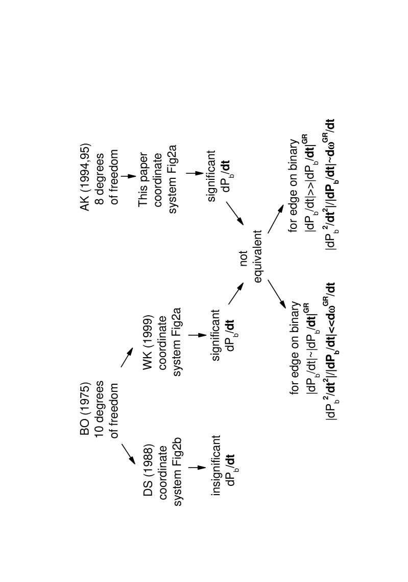
Figure 4: The relationship of the three kinds of S-L coupling induced orbital effects.

Obviously, if Damour $\&$ Schäfer’s $\dot{\omega}$ is also calculated in the coordinate system as that of Wex $\&$ Kopeikin, then Eq(81) reduces to Eq(79). Thus, the discrepancy between Damour $\&$ Schäfer (1988) and Wex $\&$ Kopeikin (1999) is that the former calculated in a coordinate systems which is not at rest to SSB; whereas, the latter is at rest to SSB. On the other hand, the discrepancy between Wex $\&$ Kopeikin (1999) and this paper is different degrees of freedom used in the calculation of equation of motion of a binary system. The relationship of the three kinds of S-L coupling effects is shown in Fig 4.

7 Confrontation with observation

The precise timing measurement on two typical binary pulsars, PSR J2051-0827 and PSR J1713+0747, provides evidence on whether $\dot{\omega}^{S}$ and $\dot{P}_{b}$ is 1PN or 1.5PN, but it still difficult to distinguish which 1PN effect is valid, Wex $\&$ Kopeikin (1999) or this paper.

The orbital motion causes a delay of $T={\bf r}_{1}\cdot{\bf K}_{0}/c=r_{1}(t)\sin\omega^{\rm obs}(t)\sin i(t)/c$ in the pulse arrival time, where ${\bf r}$ is the pulsar position vector and ${\bf K}_{0}$ is the unit vector of the line of sight. The residual $\delta T={\bf r}_{1}\cdot{\bf K}_{0}/c-({\bf r}_{1}\cdot{\bf K}_{0}/c)_{K}$ of the time delay compared with the Keplerian value is of interest (Lai et al.  lai (1995)). Averaging over one orbit $r\approx a$, and in the case $t\ll 1/|\dot{\omega}^{\rm obs}|$, the S-L coupling induced residual is,

$$\delta T=\frac{a_{p}}{c}\cos i\frac{di}{dt}t\sin\omega^{\rm obs}+\frac{\dot{a}_{p}\sin i}{c}t\sin\omega^{\rm obs}+\frac{a_{p}\sin i}{c}\dot{\omega}^{\rm obs}t\cos\omega^{\rm obs}$$

$$=\dot{x}_{1}t\sin\omega^{\rm obs}+\frac{\dot{a}}{a}xt\sin\omega^{\rm obs}+\dot{\omega}^{\rm obs}xt\cos\omega^{\rm obs}\ .$$ (84)

By Eq.(94), we have ${\dot{a}}/{a}\sim J/a^{3}\sim\dot{\omega}^{\rm obs}$, therefore, the second and third term at the right hand side of Eq.(84) cannot be distinguished in the current treatment of pulsar timing. In other words, the effect of $\dot{a}$ can be absorbed by $\dot{\omega}^{\rm obs}$.

7.1 PSR J2051-0827

As discussed above, the second term at the right hand side of Eq.(65) can be absorbed by $\dot{\omega}^{\rm obs}$, therefore $\dot{x}\approx\dot{x}_{1}$, and by Eq.(63), we have

$$\dot{\Omega}=-\frac{\dot{x}}{x}\frac{\tan i}{\sin\lambda_{LJ}\sin\Omega_{0}}=-\frac{di}{dt}\frac{1}{\sin\lambda_{LJ}\sin\Omega_{0}}\ \ .$$ (85)

According to optical observations, the system is likely to be moderately inclined with an inclination angle $i\sim 40^{\circ}$ (Stappers et al. 2001). By the measured results of $x=0.045\,$s, $\dot{x}=-23(3)\times 10^{-14}$ (Doroshenko et al. 2001), and by assuming $\sin\lambda_{LJ}\sin\Omega_{0}=2\times 10^{-3}$, Eq.(85) can be written in magnitude,

$$\dot{\Omega}=(\frac{\dot{x}}{2.3\times 10^{-13}})(\frac{x}{0.045})^{-1}(\frac{\tan i}{\tan 40^{\circ}})(\frac{\sin\lambda_{LJ}\sin\Omega_{0}}{2\times 10^{-3}})^{-1}\sim 2\times 10^{-9}\,(\rm s^{-1})\ \ .$$ (86)

In the following estimation of this section all values are absolute values. By Eq.(57), we can assume $\ddot{\omega}^{S}\sim(\dot{\omega}^{S})^{2}\sim\dot{\Omega}^{2}\approx 4\times 10^{-18}$. Usually $\ddot{\omega}^{S}$ can vary in a large range, i.e., $\ddot{\omega}^{S}>(\dot{\omega}^{S})^{2}$, depending on different combination of parameters, such as binary parameters, magnitude and orientation of $S_{1}$ and $S_{2}$. In this paper we assume that $\ddot{\omega}^{S}\sim(\dot{\omega}^{S})^{2}$. Thus from Eq.(75) we have,

$$\dot{P}_{b}=\frac{1}{2\pi}(\frac{\ddot{\omega}^{S}}{4\times 10^{-18}})(\frac{{P}_{b}}{0.099\,{\rm d}})^{2}\sim 5\times 10^{-11}({\rm s\,s^{-1}})\ \ .$$ (87)

By Eq.(70), we can estimate $d^{3}{\omega}^{S}/dt^{3}\sim{\dot{\Omega}}^{3}\approx 8\times 10^{-27}\,$s^-3, similarly, we can estimate $d^{4}\omega^{S}/dt^{4}\sim\dot{\Omega}^{4}\approx 16\times 10^{-36}\,$s^-4.

Therefore, by Eq.(76) and Eq.(77) we have $\ddot{P}_{b}\sim 9\times 10^{-20}\,$s^-1 and $d^{3}{P}_{b}/dt^{3}\sim 2\times 10^{-28}\,$s^-2. By Eq.(65) and Eq.(66), $\ddot{x}/\dot{x}\sim\dot{\Omega}\sim 2\times 10^{-9}$s^-1, which is consistent with observation as shown in Table 2.

Therefore, once $\dot{x}$ is in agreement with the observation, the corresponding $\dot{\omega}^{S}$ can make the derivatives of $P_{b}$ be consistent with observation as shown in Table 2. Whereas, the effect derived from Damour $\&$ Schäfer’s equation cannot explain the significant derivatives of ${P}_{b}$.

7.2 PSR J1713+0747

By the measured parameters, $x=32.3\,$s, $|\dot{x}|=5(12)\times 10^{-15}$, $i=70^{\circ}$ (Camilo et al. 1994), and by assuming $\sin\lambda_{LJ}\sin\Omega_{0}=1\times 10^{-4}$, then in magnitude we have,

$$\dot{\Omega}=(\frac{\dot{x}}{5\times 10^{-15}})(\frac{x}{32.3})^{-1}(\frac{\tan i}{\tan 70^{\circ}})(\frac{\sin\lambda_{LJ}\sin\Omega_{0}}{1\times 10^{-4}})^{-1}\sim 4\times 10^{-12}({\rm s^{-1}})\ \ ,$$ (88)

similarly we have,

$$\dot{P}_{b}=\frac{1}{2\pi}(\frac{\ddot{\omega}^{S}}{16\times 10^{-26}})(\frac{{P}_{b}}{67.8\,{\rm d}})^{2}\sim 1\times 10^{-10}({\rm s\,s^{-1}})\ \ .$$ (89)

The comparison of observational and predicted variabilities are shown Table 3, which are well consistent. Notice that $\dot{x}^{\rm obs}$ and $\dot{P}_{b}^{\rm obs}$ measured in these two typical binary pulsars cannot be interpreted by the gravitational radiation induced $\dot{x}$ and $\dot{P}_{b}$, since they are 3 or 4 order of magnitude smaller than those of the observational ones.

7.3 PSRs J0737-3039A and B

PSRs J0737-3039A and B is a double-pulsar system with $P_{b}=0.102251563(1)$day, advance of periastron, $\dot{\omega}=16.90(1)$deg/yr and orbital inclination angle $i=87.7^{+17}_{-29}$ (Burgay et al. 2003, Lyne et al. 2004). This binary pulsar system with $i\approx\pi/2$ may tell us not only whether $\dot{\omega}^{S}$ and $\dot{P}_{b}$ is significant or not, but also which significant $\dot{\omega}^{S}$ and $\dot{P}_{b}$ effects (Wex $\&$ Kopeikin or this paper) is valid.

As given by Eq.(69) the measured $\dot{\omega}$ is the sum of relativistic advance of periastron and the S-L coupling induced advance of periastron,

$$\dot{\omega}^{\rm obs}=\dot{\omega}^{GR}+\dot{\omega}^{S}=16.90\ (deg/yr)\ \,.$$ (90)

$\dot{\omega}^{GR}$ and $\dot{\omega}^{S}$ are both 1PN. In order of magnitude one can estimate

$$\dot{\omega}^{S}\sim\dot{\omega}^{\rm obs}=16.90\ (deg/yr)\ \,.$$ (91)

Thus we have $\ddot{\omega}^{S}\sim(\dot{\omega}^{S})^{2}\approx 8.8\times 10^{-17}$s^-2. By the same treatment of PSR J2051-0827 and PSR J1713+0747 we have,

$$\dot{P}_{b}=\frac{1}{2\pi}(\frac{\ddot{\omega}^{S}}{8.8\times 10^{-17}})(\frac{{P}_{b}}{0.1\,{\rm d}})^{2}\sim 1\times 10^{-9}({\rm s\,s^{-1}})\ \ .$$ (92)

The treatment $\dot{\omega}^{S}\sim\dot{\omega}^{\rm obs}$ and $\ddot{\omega}^{S}\sim(\dot{\omega}^{S})^{2}$ might over estimate the S-L coupling induced $\dot{P}_{b}$ for one or even two order of magnitude. Nevertheless, the S-L coupling induced $\dot{P}_{b}$ is likely much larger than that caused by the gravitational radiation, $\dot{P}_{b}^{GR}=-1.2\times 10^{-12}$ ${\rm s\,s^{-1}}$ (Burgay et al. 2003). Since the observational $\dot{P}_{b}$ will be given soon(Burgay et al. 2003), whether $\dot{P}_{b}$ is significant or not can be tested on this binary pulsar system.

The specific orbital inclination of this binary pulsar system can tell us more about the S-L coupling induced effects. By $i=87.7^{+17}_{-29}$ of PSRs J0737-3039A and B, we have $\cot i\approx 0.04$, therefore Wex and Kopeikin’s $\dot{\omega}^{S}$ given by Eq.(79) should be much smaller than that of this paper’s $\dot{\omega}^{S}$ given by Eq.(78).

Thus we have two ways to test the validity the S-L coupling effect given by Wex and Kopeikin (1999) and this paper.

The first one is that by $\ddot{\omega}^{S}\sim(\dot{\omega}^{S})^{2}\propto(\cot i)^{2}$, and $\dot{P}_{b}\propto(\dot{\omega}^{S})^{2}$, we have $(\dot{P}_{b})_{WK}\sim(\cot i)^{2}\dot{P}_{b}$. Thus the magnitude of $\dot{P}_{b}$ corresponding to Wex and Kopeikin should not exceed $1.6\times 10^{-12}$ ${\rm s\,s^{-1}}$, which is close to gravitational wave induced $\dot{P}_{b}$.

In other words if the measured magnitude of $\dot{P}_{b}$ of PSRs J0737-3039A and B is not much larger than that gravitational wave induced $\dot{P}_{b}$, then the expression of this paper can be excluded.

The second one is based on Eq.(75) to Eq.(77), from which we have,

$$\frac{|\ddot{P}_{b}|}{|d^{3}{P}_{b}/dt^{3}|}\sim\frac{|\dot{P}_{b}|}{|\ddot{P}_{b}|}\sim\frac{1}{|\dot{\omega}^{S}|}$$ (93)

Since $\dot{\omega}^{S}$ corresponds to Wex and Kopeikin is nearly two order of magnitude smaller than the relativistic advance of periastron, $\dot{\omega}^{GR}$; whereas, $\dot{\omega}^{S}$ of this paper is same order of magnitude of $\dot{\omega}^{GR}$. Therefore, if the ratio of Eq.(93) is close to $1/\dot{\omega}^{GR}$ then this paper is supported.

The precise measurement of derivatives of ${P}_{b}$ of this binary pulsar system may provide chance to test which one is favored.

8 Discussion and conclusion

BO and AK’s orbital precession velocity has been treated as equivalent, since BO and AK give equivalent torque, $\dot{\bf L}$, as shown in Eq.(9) and Eq.(18) respectively. However Eq.(9) and Eq.(18) actually correspond to two different orbital precession velocities, Eq.(12) and Eq.(19) respectively, this is because the same torque can cause different effect when a dynamic system is calculated under different degrees of freedom. BO’s orbital precession velocity is actually obtained under 10 degrees of freedom; whereas, AK’s is under 8 degrees of freedom. Correspondingly the former one violates the triangle constraint and the latter one satisfies it.

The discrepancy in physics results discrepancy in observation. Eq.(12) and Eq.(19) correspond to different combinations of $\Omega$ and $\omega$ ($\Omega$ and $\omega$ are defined in Fig.2), and since observational effect depends on $\Omega$ and $\omega$ instead of $\dot{\bf L}$, therefore, the equivalent value in $\dot{\bf L}$ may correspond to different observational effects. Concretely, BO and AK give same $\Omega$, but different $\omega$ (notice that $\Omega$ and $\omega$ are components of the vectors given by Eq.(12) or Eq.(19)). And by Eq.(67) and Eq.(68), the observed advance of precession of periastron depends on both $\Omega$ and $\omega$, thus BO and AK must correspond to different observational effects.

In the calculation of Sect 4 and Sect 5, we can see the influence of the degree of freedom and physical constraint on the results of equation of motion, perturbation and observational effects.

The S-L coupling induced precession of orbit can cause an additional time delay to the time of arrivals (TOAs), which can be absorbed by the orbital period. And since the additional time delay itself is a function of time, therefore orbital period change, $\dot{P}_{b}$, appears. Actually $\dot{P}_{b}$ corresponds to $\ddot{\omega}^{S}$ as shown in Eq.(75), which cannot be absorbed by $\dot{\omega}^{GR}$ ($\dot{\omega}^{S}$ can be absorbed by $\dot{\omega}^{GR}$). Therefore, the higher order of derivatives of orbital period provide good chance to test different models. The observation of $\dot{P}_{b}$, $\ddot{P}_{b}$ and $d^{3}{P}_{b}/dt^{3}$ on PSR J 2051-0827 supports significant S-L coupling induced effects.

This paper for the first time points out that Wex $\&$ Kopeikin’s expression in 1999 actually corresponds to significant $\dot{\omega}^{S}$ and $\dot{P}_{b}$, however it is not equivalent to the significant $\dot{\omega}^{S}$ and $\dot{P}_{b}$ given by this paper. Precise measurement of $\dot{P}_{b}$, $\ddot{P}_{b}$ and $d^{3}{P}_{b}/dt^{3}$ of specific binary pulsars with orbital inclination $i\rightarrow\pi/2$, like PSRs 0737-3039A and B, may provide chance to test the validity of the results corresponding to Wex $\&$ Kopeikin (1999) and that of this paper.

9 Appendix

By $\widetilde{S}={\bf a}_{so}\cdot\hat{\bf n}$ and $T={\bf a}_{so}\cdot\hat{\bf t}$, $\frac{d\Omega}{dt}$ and $\frac{d\omega}{dt}$ have been given by Eq.(49), Eq.(50), Eq.(55), and Eq.(57), following the standard procedure for computing perturbations of orbital elements Roy (roy (1991)). Similarly, four other elements can be given:

$$\frac{da}{dt}=\frac{2}{n\sqrt{1-e^{2}}}(\widetilde{S}e\sin f+\frac{p\widetilde{T}}{r})\ \,,$$ (94)

$$<\frac{da}{dt}>=\frac{4\sigma_{1}J(1+e^{2})}{(1-e^{2})^{5/2}a^{2}}(P_{x}Q_{y}-P_{y}Q_{x})\ \,,$$ (95)

$$\frac{de}{dt}=\frac{\sqrt{1-e^{2}}}{na}[\widetilde{S}\sin f+\widetilde{T}(\cos E+\cos f)]\ \,,$$ (96)

$$<\frac{de}{dt}>=\frac{4\sigma_{1}Je}{(1-e^{2})^{3/2}a^{3}}(P_{x}Q_{y}-P_{y}Q_{x})\ \,,$$ (97)

$$\frac{d\lambda_{LJ}}{dt}=\frac{\widetilde{W}r\cos(\omega+f)}{na^{2}\sqrt{1-e^{2}}}\frac{1}{\sin\lambda_{LJ}}\ ,$$ (98)

$$<\frac{d\lambda_{LJ}}{dt}>=\frac{3\cos\lambda_{LJ}}{2a^{3}(1-e^{2})^{3/2}\sin\lambda_{LJ}}(P_{z}\cos\omega+Q_{x}\sin\omega)[(P_{y}Q_{z}-P_{z}Q_{y})(S_{x}\sigma_{1}+S_{2x}\sigma_{2})$$

$$+(P_{z}Q_{x}-P_{x}Q_{z})(S_{y}\sigma_{1}+S_{2y}\sigma_{2})+(P_{x}Q_{y}-P_{y}Q_{x})(S_{z}\sigma_{1}+S_{2z}\sigma_{2})]\ ,$$ (99)

$$\frac{d\epsilon}{dt}=\frac{e^{2}}{1+\sqrt{1-e^{2}}}\frac{d\varpi}{dt}+2\frac{d\Omega}{dt}(1-e^{2})^{1/2}(\sin^{2}\frac{\lambda_{LJ}}{2})-\frac{2r\widetilde{S}}{na^{2}}\ ,$$ (100)

where $\frac{d\varpi}{dt}=\frac{d\omega^{\prime}}{dt}+2\frac{d\Omega}{dt}(\sin^{2}\frac{\lambda_{LJ}}{2})$.

$$<\frac{d\epsilon}{dt}>=\frac{e^{2}}{1+\sqrt{1-e^{2}}}<\frac{d\varpi}{dt}>+2<\frac{d\Omega}{dt}>(1-e^{2})^{1/2}(\sin^{2}\frac{\lambda_{LJ}}{2})$$

$$-\frac{4\sigma_{1}J}{a^{3}(1-e^{2})}(P_{x}Q_{y}-P_{y}Q_{x})\ .$$ (101)

Table 1: Comparison of S-L coupling induced variabilities given by different authors

	DS (1988)	WK (1999)	This paper	evidence
$\dot{\Omega}$ in J-co		1PN	1PN
$\dot{\omega}$ in J-co		1PN	1.5PN
$\dot{\omega}^{\rm S}$	$\sim\dot{\Omega}_{S}$ (of Eq.(12))	$-\dot{\lambda}_{LJ}\cot i\sin\Omega$	$\dot{\Omega}-\dot{\lambda}_{LJ}\cot i\sin\Omega$
$\dot{\omega}^{\rm obs}$	$\dot{\omega}^{GR}$+1.5PN	$\dot{\omega}^{GR}$+1PN	$\dot{\omega}^{GR}$+1PN
$\dot{P}_{b}$	$\dot{P}_{b}^{GR}$	$|\dot{P}_{b}^{\rm obs}|\gg|\dot{P}_{b}^{GR}|$	$|\dot{P}_{b}^{\rm obs}|\gg|\dot{P}_{b}^{GR}|$	$|\dot{P}_{b}^{\rm obs}|\gg|\dot{P}_{b}^{GR}|$
when $i\rightarrow\pi/2$		$\dot{P}_{b}^{obs}\rightarrow\dot{P}_{b}^{GR}$	$|\dot{P}_{b}^{obs}|\gg|\dot{P}_{b}^{GR}|$

J-co represents J-coordinate system, $\dot{P}_{b}^{GR}$ represents orbital period change due to gravitational radiation predicted by General Relativity. $\dot{\Omega}_{S}$ is given by Eq.(12) which is 1.5PN, whereas, $\dot{\Omega}$ and $\dot{\lambda}_{LJ}$ are 1PN, as given by Eq.(50) and Eq.(98) respectively.

Table 2: Measured parameters compared with the geodetic precession induced ones in PSR J2051$-$0827

observation	WK $\&$ this paper
$\dot{x}^{\rm obs}\approx-23(3)\times 10^{-14}$	$\dot{x}=\dot{x}^{\rm obs}$
$({\ddot{x}}/{\dot{x}})^{\rm obs}\leq-3.0\times 10^{-9}$s-1	$|{\ddot{x}}/{\dot{x}}|\approx 2\times 10^{-9}$s-1
$\dot{P}_{b}^{\rm obs}=-15.5(8)\times 10^{-12}$	$|\dot{P}_{b}|=|\frac{\ddot{\omega}^{S}P_{b}^{2}}{2\pi}|\sim 5\times 10^{-11}$
$\ddot{P}_{b}^{\rm obs}=2.1(3)\times 10^{-20}$s-1	$|\ddot{P}_{b}|=|\frac{P_{b}^{2}}{2\pi}\frac{d^{3}{\omega}^{S}}{dt^{3}}|\sim 9\times 10^{-20}$s-1
$\frac{d^{3}{P}_{b}^{\rm obs}}{dt^{3}}=3.6(6)\times 10^{-28}$s-2	$|\frac{d^{3}{P}_{b}}{dt^{3}}|=|\frac{P_{b}^{2}}{2\pi}\frac{d^{4}{\omega}^{S}}{dt^{4}}|\sim 2\times 10^{-28}$s-2

Table 3: Measured parameters compared with the geodetic precession induced ones in PSR J1713+0747

observation	WK $\&$ this paper
$|\dot{x}|^{\rm obs}=5(12)\times 10^{-15}$	$\dot{x}=\dot{x}^{\rm obs}$
$\dot{P}_{b}^{\rm obs}=1(29)\times 10^{-11}$	$|\dot{P}_{b}|=|\frac{\ddot{\omega}^{S}P_{b}^{2}}{2\pi}|\sim 1\times 10^{-10}$

Figure 1: In 1PN, the scenario of motion of a binary pulsar system can be described as the rotation of the plane determined by ${\bf L}$, ${\bf S}$ around the fixed axis, ${\bf J}$. $\eta_{L}$ and $\eta_{S}$ are precession phases of ${\bf L}$ and ${\bf S}$ in the J-coordinate system respectively.

Figure 2: Fig 2a: binary geometry and definitions of angles of Wex $\&$ Kopeikin (1999) and this paper. The invariable plane (x-y), as represented by the dotted ellipse, is perpendicular to the total angular momentum, ${\bf J}$. The inclination of the orbital plane with respect to the invariable plane is $\lambda_{LJ}$, which is also the precession cone angle of ${\bf L}$ around ${\bf J}$. The orbital inclination with respect to the line of sight is $i$. $\Omega$ is the longitude of the ascending node. $\omega$ is the longitude of the periastron from point B, and $\dot{\omega}^{\rm obs}$ is longitude of the periastron from point A. The J-coordinate system is determined by ($x$, $y$, $z$), and the observer’s coordinate system is determined by ($x^{\prime}$, $y^{\prime}$, $z^{\prime}$). Fig 2b: coordinate system of Damour $\&$ Schäfer (1988), which is determined by triad ($\hat{\bf L}$, ${\bf i}$, ${\bf K}_{0}$). ii in Fig 2b represents ${\bf i}$.

Figure 3: Angles and orientation conventions relating vectors ${\bf S}$, ${\bf L}$ and ${\bf J}$ to the coordinate system. x-y is the invariance plane, $\eta_{S1}$, $\eta_{S2}$, $\eta_{S}$ and $\eta_{L}$ are precession phases of ${\bf S}_{1}$, ${\bf S}_{2}$, ${\bf S}$ and ${\bf L}$, respectively.

References

• (1) Apostolatos,T.A., Cutler, C., Sussman,J.J. Thorne,K.S., 1994, Phys. Rev. D, 49, 6274–6297 .
• (2) Barker,B.M., O’Connell, R.F., 1975, Phys. Rev. D, 12, 329–335.
• (3) Burgay, M. et al. 2003, Nature, 426, 531. Astrophys. J. 437, L39–L42 .
• (4) Camilo, F., Foster, R.S., Wolszczan, A., 1994, Astrophys. J. 437, L39–L42 .
• (5) Damour, T., Schäfer, G., 1988 IL Nuovo Cimento, 101B, 127 .
• (6) Doroshenko,O., Löhmer, O., Kramer, M., Jessner, A., Wielebinski,R., Lyne,A.G., Lange, Ch., 2001, Astro-Astrophys, 379, 579–588 .
• (7) Hamilton, A.J.S.  Sarazin, C.L., 1982, MNRAS 198, 59–70 .
• (8) Kidder, L.E., 1995, Phys. Rev. D, 52, 821–847.
• (9) Kopeikin, S.M., 1996, Astrophys. J. 467, L93–L95.
• (10) Lai, D., Bildsten, L., Kaspi,V., 1995, Astrophys. J. 452, 819–824 .
• (11) Liu, L., 1993, Method in Celestial Mechanics, Nanjing University Press
• (12) Lyne, A. G. et al. 2004, Science, 303, 1153.
• (13) Roy, A.E., 1991, Orbital motion, Adam Hilger
• (14) Smarr, L.L.,Blandford, R.D., 1976, Astrophys. J. 207, 574–588.
• (15) Stappers, B.W. , Van Kerkwijk,M.H., Bell, J.F., Kulkarni, S.R., 2001, Astrophys. J. 548, L183–L186 .
• (16) Wex, N., Kopeikin, S.M., 1999, Astrophys. J. 514, 388.
• (17) Yi, Z.H., 1993, Essential Celestial Mechanics, Nanjing University Press