A synthetic view on structure and evolution of the Milky Way

Since the Hipparcos mission and recent large scale surveys in the optical and the near-infrared, new constraints have been obtained on the structure and evolution history of the Milky Way. The population synthesis approach is a useful tool to interpret such data sets and to test scenarios of evolution of the Galaxy. We present here new constraints on evolution parameters obtained from the Besançon model of population synthesis and analysis of optical and near-infrared star counts. The Galactic potential is computed self-consistently, in agreement with Hipparcos results and the observed rotation curve. Constraints are posed on the outer bulge structure, the warped and flared disc, the thick disc and the spheroid populations. The model is tuned to produce reliable predictions in the visible and the near-infrared in wide photometric bands from U to K. Finally, we describe applications such as photometric and astrometric simulations and a new classification tool based on a Bayesian probability estimator, which could be used in the framework of Virtual Observatories. As examples, samples of simulated star counts at different wavelengths and directions are also given.

1 Introduction

The population synthesis approach aims at assembling current scenarios of galaxy formation and evolution, theories of stellar formation and evolution, models of stellar atmospheres and dynamical constraints, in order to make a consistent picture explaining currently available observations of different types (photometry, astrometry, spectroscopy) at different wavelengths.

The validity of any Galactic model is always questionable, as it describes a smooth Galaxy, while inhomogeneities exist, either in the disc or the halo. The issue is not to make a perfect model that reproduces the known Galaxy at any scale. Rather one aims to produce a useful tool to compute the probable stellar content of large data sets and therefore to test the usefulness of such data to answer a given question in relation to Galactic structure and evolution. Modeling is also an effective way to test alternative scenarios of galaxy formation and evolution.

The originality of the Besançon model, as compared to a few other population synthesis models presently available for the Galaxy, is the dynamical self-consistency. The Boltzmann equation allows the scale height of an isothermal and relaxed population to be constrained by its velocity dispersion and the Galactic potential. The use of this dynamical constraint avoids a set of free parameters quite difficult to determine: the scale height of the thin disc at different ages. It gives the model an improved physical credibility.

In section 2, we show how the model describes the Galactic populations, as they are accounted for in the model and how constraints on galaxy evolution are incorporated. In section 3 we describe current and future applications of such a model and give a sample of comparisons between model predictions and existing data. In section 4 we discuss ongoing plans and future improvements.

2 Galactic populations and Galaxy evolution

The scenario of evolution of the Galaxy slightly evolves as new data become available (new wavelengths, deeper samples, more accurate observations, …), and as physical processes are better understood. Model predictions have to be checked and eventually model parameters have to be refined. One should always take care that the model stays self-consistent and that the overall agreement is conserved. In this section we describe the overall inputs in an up-to-date model of the Galaxy, how accurately the physical parameters are constrained, and which data are used to constrain them. This results in a description of the Galactic populations consistent with the current scenario of Galaxy evolution.

The main scheme of the model is to reproduce the stellar content of the Galaxy, using some physical assumptions and a scenario of formation and evolution. We essentially assume that stars belong to four main populations : the thin disc (sect.2.1), the thick disc (sec.2.2), the stellar halo (or spheroid, sect. 2.3), and the outer bulge (sect. 2.4). White dwarfs are taken into account separately but self-consistently (sect. 2.5). A model of distribution of the extinction is also assumed (sect. 2.6).

The modeling of each population is based on a set of evolutionary tracks, assumptions on density distributions, constrained either by dynamical considerations or by empirical data, and guided by a scenario of formation and evolution.

In Bienaymé et al. (1987a, b) we have shown for the first time an evolutionary model of the Galaxy where the dynamical self-consistency was taken into account to constrain the disc scale height and the local dark matter. Then Haywood et al. (1997) used improved evolutionary tracks and remote star counts to constrain the initial mass function (IMF) and star formation rate (SFR) of the disc population. The thick disc formation scenario has been studied using photometric and astrometric star counts in many directions, which also provided its velocity ellipsoid, local density, scale height, and mean metallicity. These physical constraints led to a demonstration that the probable scenario of formation was by an accretion event at early ages of the Galaxy (Robin et al., 1996).

More recently, the Hipparcos mission and large scale surveys in the optical and the near-infrared have led to new physical constraints improving our knowledge of the overall structure and evolution of the Galaxy. These new constraints, now included in the present version of the model, are presented below.

2.1 Thin disc

In the scheme of computing the population synthesis model, the stellar content at each epoch has been computed from standard parameters such as the initial mass function (IMF), a star formation rate (SFR), and a set of evolutionary tracks (see Haywood et al., 1997, and references therein). The disc population has been assumed to evolve during 10 Gyr, age derived from the white dwarf luminosity function with an accuracy of about 15% (Wood & Oswalt, 1998). Sets of IMF slopes and SFRs have been tentatively assumed and tested against star counts. The preliminary tuning of the disc evolution parameters against relevant observational data was extensively described in Haywood et al. (1997). We present below further improvements in the disc description from new observational constraints.

2.1.1 Hipparcos inputs and the dynamical self-consistency

Thanks to the Hipparcos mission, new and more accurate measurements have been made of the local density and potential (Crézé et al., 1998), luminosity function (Jahreiss & Wielen, 1997) and kinematics (Gómez et al., 1997). These new constraints have been included in the modeling as follows.

First, the new Hipparcos luminosity function is used to constrain the IMF at low masses in the solar neighbourhood. The IMF is modeled by a two-slope power law (table 1). At high masses, the slope $\alpha=3$ is slightly higher than the Salpeter assumption, as determined by Haywood et al. (1997). At the low mass end the slope has been revised to $\alpha$=1.6 (instead of 1.7 in Haywood et al. (1997)) to give a better fit to the Jahreißnew luminosity function from the revised Catalogue of Nearby Stars (2001, private communication). The new IMF slope gives a better fit to the local luminosity function in the range $6\leavevmode\nobreak\ <\leavevmode\nobreak\ M_{V}<\leavevmode\nobreak\ 13$ as shown in figure 1. At the lower luminosity end, the local sample is still too poor to ascertain the IMF slope. This slope is in good agreement with independent and detailed analysis from Kroupa (2000) which is in favor of a slope $\alpha=1.3\pm 0.5$ for the mass range 0.08 to 0.5 M_⊙. Kroupa adopted four different slopes in four mass ranges. Contrary to us, in the mass range 0.5 to 1.0 M_⊙, Kroupa adopts $\alpha=2.3\pm 0.3$, that is a Salpeter IMF. We estimate that presently available field data do not give enough constraints to adjust an IMF with four different slopes depending on the mass range. We have rather chosen to rely on a simpler modeling (two slopes) of the IMF for the thin disc population, until complementary constraints are available.

Figure 1: Luminosity function in the V band in the solar neighbourhood. Crosses with Poisson errors: Jahreiss determination from the revised Catalogue of Nearby Stars; Lines: model LF assuming an IMF slope of $\alpha$=1.7 (solid line) and 1.6 (dashed line) at m$<$1M_⊙.

Second, as Hipparcos has provided new constraints on the local kinematics, the age-velocity dispersion relation from Gómez et al. (1997) is introduced (cf sect. 2.1.4).

Third, the local density of interstellar matter has been revised. From Dame (1993) the local surface density of HI+H₂ is about 6 M_⊙ pc^-2 with a considerable uncertainty of about a factor of 2. With a scale height estimated to 140 pc, the local mass density is 0.021 M_⊙ pc^-3. This is about half the local density used in the previous version of our model. We notice however that the uncertainty is still very large.

Adding up the mass density from stars, interstellar matter and local contribution of the dark halo (see table 2), we end up with a total local mass density of 0.0759 M_⊙ pc^-3, in agreement with the dynamical value 0.076 $\pm 0.015\mbox{\rm M${}_{\odot}$}\mathrm{pc}^{-3}$ obtained by Crézé et al. (1998) from a detailed analysis of the K_z force on a sample of A and F stars observed by Hipparcos.

Table 1: Age, metallicity ($[\frac{Fe}{H}]$) (mean and dispersion about the mean), radial metallicity gradient (dex/kpc), initial mass function (IMF), and star formation rate (SFR) of the stellar components.

	Age (Gyr)	$[\frac{Fe}{H}]$ (dex)	$\frac{d[Fe/H]}{dR}$	IMF	SFR
Disc	0-0.15	0.01 $\pm$ 0.12
	0.15-1	0.03 $\pm$ 0.12
	1-2	0.03 $\pm$ 0.10		dn/dm $\propto$ m-α
	2-3	0.01 $\pm$ 0.11	$-$0.07	$\alpha$ = 1.6 for m $<1\mbox{\rm M${}_{\odot}$}$	constant
	3-5	$-$0.07 $\pm$ 0.18		$\alpha$ = 3.0 for m $>1\mbox{\rm M${}_{\odot}$}$
	5-7	$-$0.14 $\pm$ 0.17
	7-10	$-$0.37 $\pm$ 0.20
Thick disc	11	$-$0.78 $\pm$ 0.30	0.00	dn/dm $\propto$ m-0.5	one burst
Stellar halo	14	$-$1.78 $\pm$ 0.50	0.00	dn/dm $\propto$ m-0.5	one burst
Bulge	10	0.00 $\pm$ 0.40	0.00	dn/dm $\propto$ m-2.35 for m $>0.7\mbox{\rm M${}_{\odot}$}$	one burst

Table 2: Local mass density $\rho_{0}$ of the stellar components, the dark matter halo and the interstellar medium (ISM). $W$-velocity dispersion $\sigma_{W}$ used for the dynamical self-consistency, and disc axis ratios $\epsilon$ resulting from this process. The white dwarf mass density is computed assuming a white dwarf mass of 0.6M_⊙.

	Age	$\rho_{0}$	$\sigma_{W}$	$\epsilon$
	(Gyr)	($\mbox{\rm M${}_{\odot}$}\mathrm{pc}^{-3}$)	(km s${}^{-1})$
Disc	0-0.15	4.0$\times$10-3	6	0.0140
	0.15-1	7.9$\times$10-3	8	0.0268
	1-2	6.2$\times$10-3	10	0.0375
	2-3	4.0$\times$10-3	13.2	0.0551
	3-5	5.8$\times$10-3	15.8	0.0696
	5-7	4.9$\times$10-3	17.4	0.0785
	7-10	6.6$\times$10-3	17.5	0.0791
	WD	3.96$\times$10-3
Thick disc	11	1.34$\times$10-3
	WD	3.04$\times$10-4
Stellar halo	14	9.32$\times$10-6		0.76
Dark matter halo		9.9$\times$10-3		1.
ISM		2.1$\times$10-2

The evolution model gives the present distribution of stars in a column of unit volume centered on the sun as a function of intrinsic parameters (age, mass, effective temperature, gravity, metallicity). Since the evolution model does not yet account for orbit evolution, we redistribute the stars in the reference volume over the $z$ axis according to the age/thickness relation deduced from the Boltzmann equation.

Table 3: Density laws and associated parameter of the stellar components. $a^{2}=R^{2}+\frac{z^{2}}{\epsilon^{2}}$ where $R$ is the galactocentric distance, $z$ is the height above the Galactic plane, and $\epsilon$ is the axis ratio. Values of $\epsilon$ are given in table 2. The disc density law is given here without the warp and flare. The corrections for these structures are given in the text (sect. 2.1.3). d₀ are normalization constants. For the bulge, x,y and z are in the bulge reference frame and values of N, ${x_{0}},y_{0},z_{0}$ and $R_{c}$ are given in the text (sect. 2.4).

	density law
Disc	$\rho_{0}/d_{0}\times\{\exp(-(a/h_{R_{+}})^{2})-\exp(-(a/h_{R_{-}})^{2})\}$	if age $\leq$ 0.15 Gyr
	with $h_{R_{+}}$ = 5000 pc, $h_{R_{-}}$ = 3000 pc
	$\rho_{0}/d_{0}\times\{\exp(-(0.5^{2}+a^{2}/h_{R_{+}}^{2})^{1/2})-\exp(-(0.5^{2}+a^{2}/h_{R_{-}}^{2})^{1/2})\}$	if age $>$ 0.15 Gyr
	with $h_{R_{+}}$ = 2530 pc, $h_{R_{-}}$ = 1320 pc
Thick disc	$\rho_{0}/d_{0}\times\exp{(-\frac{R-R_{\odot}}{h_{R}})}\times(1-\frac{1/h_{z}}{x_{l}\times(2.+x_{l}/h_{z})}\times z^{2})$	if $|z|\leq x_{l}$, $x_{l}$=400 pc
	$\rho_{0}\times\exp{(-\frac{R-R_{\odot}}{h_{R}})}\times\frac{\exp(x_{l}/h_{z})}{1+x_{l}/2h_{z}}\exp({-\frac{|z|}{h_{z}})}$	if $|z|>x_{l}$
	with $h_{R}$ = 2500 pc, $h_{z}$ = 800 pc
Spheroid	$\rho_{0}/d_{0}\times(\frac{a_{c}}{R_{\odot}})^{-2.44}$	if $a\leq a_{c}$, $a_{c}$ = 500 pc
	$\rho_{0}\times(\frac{a}{R_{\odot}})^{-2.44}$	if $a>a_{c}$
Bulge	$N\times\exp(-0.5\times r_{s}^{2})$	$\sqrt{x^{2}+y^{2}}<R_{c}$
	$N\times\exp(-0.5\times r_{s}^{2})\times\exp(-0.5(\frac{\sqrt{x^{2}+y^{2}}-R_{c}}{0.5})^{2})$	$\sqrt{x^{2}+y^{2}}>R_{c}$
	with $r_{s}^{2}=\sqrt{[(\frac{x}{x_{0}})^{2}+(\frac{y}{y_{0}})^{2}]^{2}+(\frac{z}{z_{0}})^{4}}$
ISM	$\rho_{0}\times exp(-\frac{R-R_{\odot}}{h_{R}})\times exp(-\frac{|z|}{h_{z}})$
	with $h_{R}$ = 4500 pc, $h_{z}$ = 140 pc
Dark halo	$\frac{\rho_{c}}{(1.+(a/R_{c})^{2})}$ with $R_{c}$ = 2697 pc and $\rho_{c}$ = 0.1079

With these new inputs, the dynamical self-consistency process is applied as first described in Bienaymé et al. (1987a): assuming that the Galactic potential is given by the sum of the stellar populations (those in the present model), and adding up the interstellar matter and the dark matter halo, we compute the potential through the Poisson equation. The disc is not modeled with a double exponential but with Einasto laws (Einasto, 1979), ensuring continuity and derivability in the Galactic plane. The formulae are given in table 3. The thin disc population is sliced into seven isothermal populations of different ages, from 0 to 10 Gyr. Each sub-population (except the youngest one, which cannot be considered relaxed) has its velocity dispersion imposed by the age/velocity dispersion relation. Then using equation 1 we compute its scale height (or axis ratio in case of ellipsoids), while the rotation curve constrains the shape and local density of the dark matter halo (Bienaymé et al., 1987a).

$$\frac{\rho(z)}{\rho(0)}=\mbox{exp}\left(-\frac{\Delta\Phi}{\sigma_{W}^{2}}\right)$$ (1)

A new total mass density is then computed. The process is iterated until the values of the potential and the disc thicknesses change by less than 1%. The resulting disc axis ratios $\epsilon$ are given in table 2. The rotation curve of the best fit model is shown in figure 2.

The local density of the dark matter halo amounts to $9.9\leavevmode\nobreak\ \times\leavevmode\nobreak\ 10^{-3}$ M_⊙pc^-3, about 20% higher than the value determined by Bienaymé et al. (1987a), while the mass density of our disc is lower. The difference comes from the fact that they included an “unseen mass disc” of local density $0.01\leavevmode\nobreak\$M_⊙pc^-3 of which existence has been definitely ruled out by Crézé et al. (1998). The dark halo serves to compensate for the lack of force coming from the disc, in order to adjust the rotation curve. This is the major massive component at galactocentric distances larger than 5 kpc. The question of the composition of this dark component is still open, probably mainly non baryonic, but not exclusively. We shall consider in sect. 2.5 the possibility of this component to be made of ancient white dwarfs.

The overall model mass density ends up with the following values: the outer bulge mass, coming from old populations in the central part of the Galaxy, is $2.03\times\leavevmode\nobreak\ 10^{10}$ M_⊙, excluding the central black hole and clusters. The mass of the interstellar matter amounts to 4.95$\times\leavevmode\nobreak\ 10^{9}$ M_⊙in our modeling. The stellar thin disc reaches a mass of 2.15$\times\leavevmode\nobreak\ 10^{10}$ M_⊙, the thick disc 3.91$\times\leavevmode\nobreak\ 10^{9}$ M_⊙and the stellar halo 2.64$\times\leavevmode\nobreak\ 10^{8}$ M_⊙(excluding eventual ancient halo white dwarfs which belong to the “dark halo”). The dark halo has a mass of 4.53$\times\leavevmode\nobreak\ 10^{11}$ M_⊙inside the sphere of 50 kpc radius. The overall Galaxy mass to R$<$50 kpc amounts to 5.04$\times\leavevmode\nobreak\ 10^{11}$ M_⊙, and 9.97$\times\leavevmode\nobreak\ 10^{11}$ M_⊙within 100 kpc. These values are in good agreement with the detailed analysis of the Galactic mass by Sakamoto et al. (2003), from the latest kinematics of Galactic satellites, halo globular clusters and horizontal branch stars, which estimates the Galactic mass to $5.5^{+0.1}_{-0.4}\times 10^{11}$ M_⊙within 50 kpc and about $10\times 10^{11}$ M_⊙within 100 kpc.

Figure 2: Circular velocity of the self-consistent model. Crosses are observational constraints from Caldwell & Ostriker (1981). Contributions from main Galactic components are also given.

The density laws resulting from self-consistent adjustments of the Galactic potential are finally used to compute the stellar content all over the Galaxy, assuming that the disc IMF and SFR at the solar neighbourhood are suitable for the entire disc population. The inferred dark matter local density is also used to compute the contribution of potential ancient white dwarfs in star counts (see sect. 2.5.3.)

2.1.2 Atmosphere models and colour estimates

The evolutionary model computes the distribution of stars in the space of intrinsic parameters: effective temperature, gravity, absolute magnitude, mass and age. This distribution transcribes the theoretical constraints coming from stellar and galactic evolution (mainly the IMF, the SFR, the evolutionary tracks, and the metallicity distributions) into observable statistics, with the use of suitable atmosphere models.

The metallicity is estimated from the age of each component, assuming an age/metallicity relation and allowing for a Gaussian dispersion about the mean. For the thin disc, we use Twarog (1980) age/metallicity distribution (mean and dispersion about the mean, see table 1). An alternative new metallicity distribution from Haywood (2001), more centered on the solar metallicity, can also be used. However important to understand the scheme of the Galaxy chemical evolution, the differences between Twarog and Haywood distributions have only marginal impact on star count predictions as far as broad photometric bands are used. Conversely, it is not possible to settle this issue with ordinary photometric star counts.

The theoretical parameters are converted into colours in various photometric systems through stellar atmosphere models corrected to fit empirical data (Lejeune et al., 1997, 1998) (the BaSeL 2.2 data base). While some uncertainties still remain in the resulting colours for extreme spectral types, the BaSeL data sets allow an efficient and consistent conversion of theoretical parameters (effective temperature, gravity and metallicity) to colors in various photometric systems. For low mass stars, synthetic colours from Baraffe et al. (1998) have been used in the near-infrared in place of Lejeune calibrations. Empirical densities, infrared luminosities and colours of giants of spectral types M7 and later are introduced following the observations of Guglielmo (1993). The mid-infrared modeling of these late M giants and AGB stars may be inaccurate. It will be revised in the near future.

At present, calibrations are available for the Johnson-Cousins UBVRIJHKL. The GAIA G magnitude can also be simulated. The Sloan SDSS and Strömgren photometric systems are planned.

2.1.3 External disc

Several studies have shown that the edge of the disc is detected at a galactocentric distance of about 14 kpc (Robin et al., 1992; Ruphy et al., 1996). However when analysing DENIS near-infrared survey data (Epchtein et al., 1997) in the Galactic plane, we have shown that the warp and flare of the external disc appear clearly in near-infrared star counts (Derrière & Robin, 2001). For a long time the warp and flares have been clearly seen in HI data (Henderson et al., 1982; Burton and te Linkel Hekkert, 1986; Burton, 1988; Diplas and Savage, 1991), in molecular clouds (Grabelsky et al., 1987; Wouterlout et al., 1990; May et al., 1997), from OB stars (Miyamoto et al., 1988; Reed, 1996) and finally in COBE data (Porcel et al., 1997; Freudenreich, 1998; Drimmel & Spergel, 2001). The existence of such a warp in old stellar populations puts constraints on the time scale of this structure. However there is evidence that the stars do not follow exactly the same warp as the gas (Djorgovski and Sosin, 1989; Porcel et al., 1997). Possible origins of the warps are still under discussion but may be resolved by suitable N-body simulations (Binney, 1992). Warps may have originated from interactions between the disc and (i) the dark halo (if angular momenta are not aligned), (ii) nearby satellite galaxies, such as the Sagittarius dwarf or the Magellanic clouds, (iii) infalling intergalactic gas. From the analysis of their angular momenta, Bailin (2003) argues that the Milky Way warp and the Sagittarius Dwarf Galaxy may be coupled. Garcia-Ruiz (2002) have studied by N-body simulations the possibility for the warp to be caused by the tides of the Magellanic Clouds. They find that neither orientation nor amplitude of the warp can be reproduced in this way. Alternatively López-Corredoira et al. (2002) propose that the warp caused by intergalactic accretion flows onto the Milky Way disc.

Despite the uncertainty on the warp’s origin, in the modeling process we have started with warp and flare parameter values close to the ones observed in the gas and molecular clouds. Then, simulations have been compared with near-infrared data from the DENIS survey in a set of relevant directions, and warp and flare parameters have been adjusted. The parameters are described below :

For the warp, a tilted ring model such as Porcel et al. (1997) is considered. When computing density laws for a warped disc, the galactocentric coordinates ($R$,$\theta$,$z$) at galactocentric radii larger that $R_{\mathrm{warp}}$, are shifted perpendicular to the plane by a value

$$z_{\mathrm{warp}}=z_{c}\cos(\theta-\theta_{\mathrm{max}})$$

with $\theta_{\mathrm{max}}$ and $z_{c}$ being respectively the direction in which the warp is maximum, and the maximum elevation of the warp at a given radius. We adopt a linear increase of the warp amplitude $z_{c}$, such as

$$z_{c}=\gamma_{\mathrm{warp}}(R-R_{\mathrm{warp}})$$

Following Burton (1988), we assume that the Sun lies approximately on the line of nodes of the warp ($\theta_{\mathrm{max}}=90^{\circ}$). We adopt an amplitude similar to Gyuk et al. (1999) ($\gamma_{\mathrm{warp}}=0.18$). Preliminary results obtained from the analysis of a part of the DENIS survey (Derrière & Robin, 2001; Derrière, 2001) indicate a best value for the starting galactocentric radius of the warp to be $R_{\mathrm{warp}}=8.4$ kpc, close to $R_{\odot}$.

As in Gyuk et al. (1999), we model the flaring of the disc by increasing the scale height by a factor $k_{\mathrm{flare}}$, beyond a galactocentric radius $R_{\mathrm{flare}}$, with

$$k_{\mathrm{flare}}=1+\gamma_{\mathrm{flare}}(R-R_{\mathrm{flare}})$$

The surface density in the flaring disc is the same as in the normal one, leading to correction factors in the density laws.

The amplitude is taken from Gyuk et al. (1999) ($\gamma_{\mathrm{flare}}=5.4\times 10^{-4}$ kpc^-1). The radius at which the disc starts flaring lies beyond the solar circle. However Derrière (2001) found that the minimum radius of the flare might depend on the longitude considered. He determined a preliminary average value of $R_{\mathrm{flare}}=9.5$ kpc which may be reconsidered when near-infrared surveys such as DENIS and 2MASS will be completely analysed.

An example of the warp and flare effects on star counts in the near infrared is shown in figure 3. Squares are DENIS K star counts on a strip crossing the plane at l=266.1^o and dashed lines are model predictions in same directions. The peak of the model predictions without warp and flare (top panel) is displaced from the data peak. The middle panel shows predictions including the warp but no flare. The Galactic warped plane is well placed but the peak is too sharp. In the bottom panel the model including both features (warp and flare) correctly reproduces the star counts.

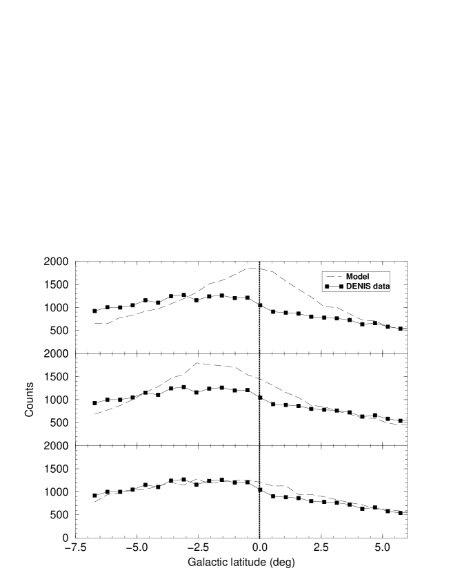
Figure 3: Star counts in K along a DENIS strip in counts per 0.8^o bin in declination (this strip crosses the plane at l=266.1^o). Data are in solid lines, models in dashed lines. Top panel: flat disc. Middle panel: warped disc. Bottom panel: warped and flaring disc.

2.1.4 Disc kinematics

The disc velocity ellipsoid is taken from Gómez et al. (1997), deduced from Hipparcos data analysis. Velocity dispersions as a function of age and galactocentric gradients are given in Table 4. The asymmetric drift is computed following the relation :

$V_{\scriptsize\mbox{ad}}=\frac{\sigma_{U}^{2}}{2V_{\scriptsize\mbox{LSR}}}\{\frac{R}{\rho}\frac{d\rho}{dR}+2\times\frac{R}{\sigma_{U}}\frac{d\sigma_{U}}{dR}+(1-\frac{\sigma_{V}^{2}}{\sigma_{U}^{2}})+(1-\frac{\sigma_{W}^{2}}{\sigma_{U}^{2}})\}$

where $\frac{d\rho}{dR}$ is the density gradient. The Sun velocities are $U_{\odot}$ = 10.3 km s^-1, $V_{\odot}$ = 6.3 km s^-1, $W_{\odot}$ = 5.9 km s^-1, and $V_{\scriptsize\mbox{LSR}}$ = 226 km s^-1. The later value is obtained after fitting the mass model to the observed rotation curve (see sect. 2.1.1). Asymmetric drift values computed at the solar position are given in table 4.

Table 4: Velocity dispersions ($\sigma_{U},\sigma_{V},\sigma_{W}$), asymmetric drift $V_{\scriptsize\mbox{ad}}$ at the solar position (see section 2.1.4) and velocity dispersion gradient $\frac{d\ln(\sigma_{U}^{2})}{dR}$, where $\sigma_{U}$ is expressed in km $s^{-1}$ and R in kpc.

	Age	$\sigma_{U}$	$\sigma_{V}$	$\sigma_{W}$	$V_{\scriptsize\mbox{ad}}$	$\frac{d\ln(\sigma_{U}^{2})}{dR}$
	(Gyr)	(km s${}^{-1})$	(km s${}^{-1})$	(km s${}^{-1})$	(km s${}^{-1})$
Disc	0-0.15	16.7	10.8	6	3.5
	0.15-1	19.8	12.8	8	3.1
	1-2	27.2	17.6	10	5.8
	2-3	30.2	19.5	13.2	7.3	$-2\times 10^{-1}$
	3-5	36.7	23.7	15.8	10.8
	5-7	43.1	27.8	17.4	14.8
	7-10	43.1	27.8	17.5	14.8
Thick disc		67	51	42	53	0
Spheroid		131	106	85	226	0
Bulge		113	115	100	79	0

2.2 Thick disc

The thick disc formation scenario that drives the model characteristics is a formation by a merger event (or several merger events) at the beginning of the life of the thin disc. This scenario well explains the observed properties of this population : The accretion body heats the stellar population previously formed in the disc making a thicker population with larger velocity dispersions. Due to the epoch of this event, the thick disc abundances are intermediate between the stellar halo and the present thin disc. Chemical abundance measurements imply that the duration of star formation in the thick disc cannot be larger than 1 Gyr (Mashonkina & Gehren, 2001). The estimated epoch of thick disc formation in the literature ranges between 8 Gyr (Ibukiyama & Arimoto, 2002) and 13 Gyr (Pettinger et al., 2001) from chemical considerations, while Quillen & Garnett (2001) find 9 Gyr from kinematics. We have finally adopted an age of 11 Gyr for this population. This is just slightly older than the thin disc, and younger than the stellar halo. The choice of the slightly different age (by 1 Gyr) would not change significantly wide band photometric star counts. Other observational constraints come from kinematics : the velocity ellipsoid and asymmetric drift have been measured by radial velocity or proper motion distributions. Ojha et al. (1996, 1999) determined the velocity ellipsoid of the thick disc from an analysis of a photo-astrometric survey in three directions at intermediate latitudes (center, anticentre, and antirotation). They found the velocity dispersions to be ($\sigma_{U},\sigma_{V},\sigma_{W}$) = (67, 51, 42) in km s^-1 with an asymmetric drift of 53 km s^-1. These values are in close agreement with a recent determination by Soubiran et al. (2003) who find a rotational lag of 51 km s^-1, and a velocity ellipsoid ($63\pm 6,39\pm 4,39\pm 4$) km s^-1. The asymmetric drift is not found to have any vertical gradient inside this population. The eventual radial gradient is still undetermined and is assumed to be zero in modeling. The absence of chemical and kinematical gradients and the large gap in properties between the thick disc and the stellar halo (scale height, rotational velocity) rule out the hypothesis that the thick disc has been formed during a dissipational collapse (Majewski, 1993) and rather favour a formation by a strong heating of a preliminary thin disc induced by a merging of a satellite onto the Galaxy (Quinn et al., 1993; Robin et al., 1996).

In order to model this population, a single epoch of star formation (that is a period of formation negligible compared to the age of the Galaxy) is assumed. Oxygen enhanced evolutionary tracks have been taken from Bergbush & VandenBerg (1992). The horizontal branch (HB) has been added following models from Dorman (1992). Stars of effective temperature between 7410 K and 6450 K are assumed to be RRLyrae. There is no blue horizontal branch, as seen on metal rich globular clusters. The position of the HB is assumed to be 3.54 visual magnitudes brighter than the main sequence turnoff.

The adopted thick disc metallicity is $-0.78$ dex, in agreement with in situ spectroscopic determination from Gilmore et al. (1995) and photometric star count determinations (Robin et al., 1996; Buser et al., 1999). The low metallicity tail of the thick disc is not taken into account, but an internal metallicity dispersion of 0.3 dex is included.

The thick disc density law has often been assumed in the literature to be exponentially decreasing perpendicular to the Galactic plane. Tests of various laws have been performed by comparing data with model predictions in various directions. At present time, it does not seem possible to obtain detailed constraints on the true shape, either exponential or sech², because the distances are not known with sufficient accuracy. Moreover the contribution of short distance stars to the star counts is often negligible due to the small volume where they are counted. We have assumed that the thick disc shape is a truncated exponential along the z axis: at large distances the law is exponential, at short distances it is a parabola (see table 3). This option ensures the continuity and derivability of the density law in the plane, to ease the computation of the thick disc contribution to the potential.

The density law parameters and IMF adopted are well constrained by the analysis of deep wide field and near-infrared star counts at high and intermediate Galactic latitudes (Reylé & Robin, 2001a). The best fit model has a scale length $h_{R}$ = 2500 $\pm$ 500 pc, a scale height $h_{z}$ = 800 $\pm$ 50 pc with $x_{l}$=400 pc, and a local density $\rho_{0}$ = 1.03$\times 10^{-3}$ stars pc^-3 or 7.6$\times 10^{-4}$ M_⊙ pc^-3 for M_V $\leq$ 8, corresponding to 6.8% of the thin disc local density. The IMF is dN/dm $\propto$ m^-0.5, the slope being also constrained by large data sets (Reylé & Robin, 2001a). The total density (excluding white dwarfs) is then 2.83$\times 10^{-3}$ stars pc^-3 or 1.34 10^-3 M_⊙ pc^-3. This value does not account for binarity. Thus the true IMF should slightly steepen. The binarity correction should play a role only in very deep star counts. Such star counts are few and they remain uncertain due to strong galaxy contamination.

2.3 Stellar halo

We here distinguish what we call the stellar halo, or spheroid, from the dark matter halo. The spheroid is distinct from the bulge in the model construction. However they may be related in their formation scenario. The spheroid, or stellar halo, is essentially old and metal poor. The bulge is also quite old but its abundance distribution is sensitively different, with a metallicity distribution closer to the one of the thick disc population. On the other hand, the stellar halo should be considered distinct from the dark matter halo, which is probably mainly non baryonic, although a small part of it can be formed of stellar remnants. We shall consider this point in sect. 2.5.3.

Mainly two possible scenarios of formation of the spheroid are competing. The first one is a dissipational collapse of pre-galactic gas, the second one being based on accretion of smaller pieces. Streams have already been found, related to known accretion events (Sagittarius galaxy, …) but the proportion of spheroid stars which can originate from such streams is still not known. Therefore our standard model assumes a homogeneous population of spheroid stars with a short period of star formation, which should be a good representation on large scales. Comparisons with true data should then, by contrast, help finding existing streams. Bergbush & VandenBerg (1992) oxygen enhanced models are used assuming a Gaussian metallicity distribution of mean -1.78 and dispersion 0.5 dex. The age of the spheroid is assumed to be 14 Gyr, a value which may be slightly high, as constrained by the analysis of the WMAP experiment (Bennett et al., 2003). However, a change by 0.5 Gyr would have no effects on star count predictions.

The density law and IMF of the spheroid were constrained using deep star counts at high and medium Galactic latitudes (Robin et al., 2000). This global adjustment of the spheroid shape has led to the following values: the density law (see table 3) is characterized by a power law index $n$ = 2.44, a flattening $\epsilon$ = 0.76 and a local density $\rho_{0}$ = 2.185$\times 10^{-5}$ pc^-3 or 0.932 10^-5 M_⊙ pc^-3 including all red dwarfs down to the hydrogen burning limit, but not the white dwarfs. This local density has been computed with an IMF dN/dm $\propto$ m^-0.5, similar to the globular clusters and to the thick disc population (see discussion below). The total local density depends a lot on the assumed IMF at low masses. With an IMF of dN/dm $\propto$ m^-2, the total local density would be $8.19\times 10^{-5}$ stars pc^-3. Model predictions are affected by the IMF slope value only at magnitudes fainter than V$=22$ at the Galactic pole (see figure 4 and sect. 4).

The relative density of the spheroid to the disc is about 0.06% when one selects stars at M${}_{V}<8$. Yet this value ignores possible old white dwarfs. The ancient white dwarf contribution will be considered separately below.

2.4 Outer bulge and disc hole

Bulge formation in the Galaxy is still an open question. Several scenarios compete to explain the observed structures. The proposed scenarios are : primordial collapse (Eggen et al., 1962), hierarchical galaxy formation (Kauffmann et al., 1994) (early merging), infall of satellite galaxies (late merging), and secular evolution of discs (starbursts induced by bar instabilities). Bouwens et al. (1999) argue that all these mechanisms could have been at work over the history of the Universe in forming bulges. Nakasato & Nomoto (2003) have performed three-dimensional hydrodynamical N-body simulations of the formation of the Galactic bulge, and they find that two groups of stars are present in the bulge, 60% of the stars originate in sub-galactic mergers, and 40% come from the inner region of the disc. The two groups are chemically distinct. Their model is able to reproduce the metallicity distribution and the velocity dispersion-metallicity relation.

The observational signatures of the bulge population are the following : the bulge is certainly triaxial. The asymmetry is seen from COBE/DIRBE near-infrared data : the bulge is brighter at positive longitudes than at negative ones. Dwek et al. (1995) and Freudenreich (1998) have fitted parametric models to the dereddened DIRBE data, but excluding low latitude regions. Binney et al. (1997), then Bissantz & Gerhard (2002) have obtained non-parametric models from the same data. The observed metallicity distribution of K giants is characterized by a wide distribution, [Fe/H] ranging from -1.2 to +0.9 dex (McWilliam & Rich, 1994). Minniti (1996) and Tiede and Terndrup (1999) have shown a clear relation between the velocity dispersion and the metallicity but this result may be due to a mixture of populations (halo, bulge and maybe thick disc) in their fields at latitudes between -6 and -8. The bulge is rotationally supported, the projected mean rotation of the bulge being of the order of $53.3\pm 0.3$ km s^-1 kpc^-1 (Tiede and Terndrup, 1999).

We here concentrate on the outer bulge, excluding the very central part of the Galaxy (inner bulge at longitude and latitude smaller than 1 deg) not yet well observationally constrained.

As a first approximation, we have started with the Dwek G2 density law (Dwek et al., 1995) and have fitted the parameters on near-infrared star counts from the DENIS survey. A detailed description of the process will be given elsewhere (Picaud et al., in preparation). Here we give the main results from this work.

The disc scale length is adjusted at the same time as the bulge parameters. The data towards the inner Galaxy clearly show a coexistence of both populations. However, since the Einasto formula for the disc accounts for a possible hole in the middle of the disc, we take the opportunity to constrain this parameter and check how the bulge and disc populations coexist or are replaced by each other as a function of Galactic radius.

The density laws are given in table 3. The fitted parameters for the disc are the scale length $h_{R_{+}}$ and the hole scale length $h_{R_{-}}$. For the bulge there are 8 fitted parameters (following Dwek notation):

• orientation angles: $\alpha$ (angle between the bulge major axis and the line perpendicular to the Sun - Galactic Center line ), $\beta$ (tilt angle between the bulge plane and the Galactic plane) and $\gamma$ (roll angle around the bulge major axis)

• scale-lengths $x_{0}$ on the major axis, $y_{0}$ and $z_{0}$ on minor axes

• normalization (star density at the center) $N$ and cut-off radius $R_{c}$.

In order to perform the Monte-Carlo simulations, the bulge luminosity function is taken from Bruzual et al. (1997) at solar metallicity and age of 10 Gyr. Alternatively Padova isochrones may be used in the future. A Salpeter IMF has been assumed (see table 1). This IMF slope seems to be well constrained for high mass and intermediate mass stars. This is however not the case at low masses, for which very deep observations inside the bulge are needed but difficult to get because of the crowding. From deep photometry obtained with the Hubble Space Telescope Holtzman et al. (1998) found a power-law mass function with a slope -2.2 for masses higher than 0.7, though close to the Salpeter IMF. At lower masses they found indications of a break in the mass function, as seen in other populations, occuring at about 0.5 to 0.7 M_⊙. However, due to incompleteness and uncertain binary corrections, they do not strongly constrain the value of the IMF slope at low masses. If we would follow the general scheme of other populations, we would have taken either the low mass slope of the disc (0.6) or that of the thick disc and stellar halo (-0.5). The constraints being still poor we have kept the one-slope Salpeter IMF for the time being.

The DENIS survey (Epchtein et al., 1997) has produced specific observations in the bulge well suited for this analysis. We have used catalogues in J (1.25 $\mu m$) and $K_{s}$ (2.15 $\mu m$) bands from a set of “batches”, specific observations made in the directions of the bulge (Simon et al, in preparation). Contrary to the strips done in the main survey, the batches are shorter in declination and easier to handle. About 100 windows of low extinction of 15’x15’ between longitudes [-8^∘, +12^∘] and latitudes [-4^∘; +4^∘] were chosen using the map of extinction from Schultheis et al. (1999). The completeness limits were carefully established in each band. Star counts in K and J-K were simulated and compared with the data between magnitude K 8.5 and 11.5 after extinction was fitted independently in each window.

The model goodness-of-fit is estimated through a maximum likelihood test. In order to explore the 10 dimensional space of parameters, sets of parameters were chosen by Monte Carlo selections, first from a uniform distribution, then from a Gaussian distribution around the maxima of likelihood. Fifty independent fits were made to test the robustness of the results.

The best fit parameters (mean of the 50 trials and dispersions about the mean) are given in table 5.

Table 5: Bulge fitted parameters. Values from Dwek et al. (1995) are mean values obtained from the 2.2 $\mu m$ DIRBE data for their G2 density law. $\alpha$, $\beta$ and $\gamma$ are orientation angles following the Dwek et al. (1995) notation. $x_{0}$,$y_{0}$, $z_{0}$ are the scale lengths in the three axes. $R_{c}$ is the cutoff radius and $N$ the central number density. The values of $\beta$ and Rc are not adjusted in the case of the Dwek et al. (1995) fitting process.

Parameter	Dwek et al. value	Error	Our fitting value	Error	Unit
$\alpha$	68.5	4.8	78.9∘	0.7	∘
$\beta$	0	-	3.5∘	0.2	∘
$\gamma$	90.7	1.5	91.3∘	1.1	∘
$x_{0}$	2.03	0.23	1.59	0.12	kpc
$y_{0}$	0.470	0.010	0.424	0.015	kpc
$z_{0}$	0.580	0.010	0.424	0.015	kpc
$R_{c}$	2.4	-	2.54	0.13	kpc
$N$	-	-	13.70	0.7	star.pc-3

Thus, we obtain a very oblate outer bulge (sometimes called a bar in the literature), almost in the Galactic Plane with an angle from the Sun - Galactic Center line of about 10 degrees, well in agreement with the result from López-Corredoira et al. (2000) who found an angle of 12 degrees from independent star count data. The axis ratios are in good agreement with the Dwek et al. (1995) determination but they found a slightly higher angle, although less constrained, between the major axis and the line of sight to the Galactic center (20${}^{\circ}\pm 10^{\circ}$) compared to ours (11.1${}^{\circ}\pm 0.7^{\circ}$). The good accuracy we achieved comes from the use of star counts, more sensitive to lower luminosity stars covering a larger depth inside the bulge and with a higher density, rather than integrated luminosities, dominated by the brightest stars, which may be biased by the deprojection.

The overall mass in this outer bulge is $2.03\pm 0.26\leavevmode\nobreak\ \times\leavevmode\nobreak\ 10^{10}\leavevmode\nobreak\ \mbox{\rm M${}_{\odot}$}$. It includes all populations, even white dwarfs which contribute to about 26%. It does not include the inner bulge or the central black hole. This value is slightly higher than the one determined by Dwek et al. (1995) from COBE data $1.3\leavevmode\nobreak\ \times\leavevmode\nobreak\ 10^{10}$M_⊙, but the latter is photometrically determined and does not account for white dwarfs.

The overall fit of the central region leads to include a noticeable hole in the thin disc, which is very common in barred galaxies. The resulting disc scale length is $h_{R_{+}}=2.53\pm 0.11$ kpc and the hole scale length $h_{R_{-}}=1.32\pm 0.14$ kpc.

The bar is considered as a separate population from the bulge, extending further away (up to l=27^∘ as seen by López-Corredoira et al. (2000)). It is being studied and is discussed elsewhere (Picaud et al., 2003).

2.5 White dwarfs

White dwarfs (WD) are the latest stage of stellar evolution. Their density is a function of the past star formation history and the initial mass function. Their luminosity function depends on the assumed cooling tracks and physical properties. In the modeling we assume all white dwarfs to be DA and use evolutionary tracks and atmosphere models from Bergeron et al. (1995), complemented by Chabrier (1999) for the very cool end, applicable to the halo. The former have been extensively compared with observations and have been shown to be reliable. The latter models still have to be checked, as very few ancient white dwarfs are known yet. However, they include the best physical constraints and are supposed to be good starting points for simulating ancient white dwarfs.

2.5.1 Thin disc

The luminosity function (LF) of disc white dwarfs is known from systematic searches in the solar neighbourhood. A good preliminary LF was obtained by Liebert et al. (1988). More recent determinations give larger local densities due to new detections of cool white dwarfs: Holberg et al. (2002) found $5.5\pm 0.8\times 10^{-3}$ star pc^-3, while Leggett et al. (1998) and Ruiz & Bergeron (2001) found a lower limit of $5.6\times 10^{-3}$ star pc^-3, and Knox et  al. (1999) $4.16\times 10^{-3}$ star pc^-3. It should be noted that these values depend a lot on the number of faintest white dwarfs detected at M${}_{V}>16$, which are only 3, and the way the luminosity function is binned. Wood & Oswalt (1998) estimated that the accuracy of the white dwarf density is about 50% on a sample of 50 objects (the number of white dwarfs known in the local sphere of 13 pc is 53).

To avoid Poisson noise from observational data, we have adopted a luminosity function based on the Wood (1992) model for a disc of 10 Gyr, with a constant star formation rate, coherent with our evolutionary model. This is well in agreement with the bright DA luminosity function from Liebert et al. (1988) and is slightly higher in the coolest part of the observed white dwarf luminosity function, allowing for incompleteness in the local sample. The total local density is then 6.6 $\times 10^{-3}$ star pc^-3 and the mass density 3.96 $\times 10^{-3}$ M_⊙ pc^-3.

2.5.2 Thick disc

The thick disc white dwarf population has been computed by Garcia-Berro (private communication and Garcia-Berro et al. (1999)) assuming a Salpeter IMF. Very few thick disc white dwarfs have yet been identified in the field. Hence, we have tentatively normalized the theoretical LF by fitting model predictions on the Oppenheimer et al. (2001) sample of high velocity white dwarfs. Reylé et al. (2001b) have shown that most of the Oppenheimer WD belong to the thick disc populations, as suggested by their kinematical properties. It gives a density of white dwarfs relative to the red dwarfs of 20% that is 5$\times 10^{-4}$ stars pc^-3.

2.5.3 Halo white dwarfs

Due to the microlensing results towards the Magellanic Clouds, the hypothesis that a significant number of ancient white dwarfs are present in the halo is seriously considered. The local contribution of this faint population in the solar neighbourhood is detectable and several studies have been conducted in order to find them. Thus, this hypothetical population has been tentatively included in the model.

The current estimation of machos density from microlensing events towards the Magellanic Clouds (Lasserre et al., 2000; Alcock et al., 2000) has an upper limit of about 20% of dark matter halo made of machos. Freese & Graff (1997) have shown the improbability of the machos to be red or brown dwarfs, leaving the possibility for ancient white dwarfs to be the lenses. These results have stimulated the search for the local counterpart of the halo baryonic dark matter in the form of white dwarfs. However, the results give a quite smaller local density : Goldman et al. (2002) have shown that the local density of halo white dwarfs cannot exceed 5% of the dark halo and Oppenheimer et al. (2001) give a lower limit of 3%, although we do not think, from their kinematics, that all Oppenheimer objects are really halo white dwarfs (Reylé et al., 2001b). Mendez (2002) has recently found a population of old white dwarfs in a proper motion survey near the globular cluster NGC6397. Among his 7 peculiar white dwarfs he claims to have a halo white dwarf and 6 thick disc white dwarfs. If he is right, then the number of thick disc white dwarfs is huge compared with the number generally assumed and they have (for 4 among 6) a surprising rotational velocity higher than the LSR, while one expects a significantly smaller rotational velocity for the thick disc population. The identification of these stars as belonging to the thick disc is then problematic. One should consider rather the possibility of them being disc white dwarfs which have undergone a kick off in a mass-transfer binary, as proposed by Bergeron (2003). Considering the Mendez’s halo white dwarf candidate, the halo white dwarf mass density inferred by this object would be about half the density of the dark halo (4.25 $\pm$ 2.8 M_⊙pc^-3) if this star is a halo object. Its proper motion is still compatible with thick disc kinematics.

Another recent search for high proper motion objects in the VIRMOS survey (Le Fèvre et al., 1998) on 0.94 square degree adding to a 0.16 square degree in the SA57 field obtained also at the CFHT produces no detection of high proper motion white dwarf in selection limits, where a 100% white dwarf halo aged 14 Gyr would place between 12.6 and 20.4 detectable objects (depending on the adopted halo IMF). This sets at the 95% probability level the upper limit of the halo fraction in the form of halo white dwarfs between 24% and 15% (Crézé et al, in preparation). The thick disc white dwarf population seen by Mendez has not been seen in this Virmos field.

Chabrier et al. (1996) have reconsidered the hydrogen white dwarf cooling sequence and recomputed their model atmosphere and color-magnitude diagrams. In order to build their luminosity function and detection probabilities, they considered two different IMFs (Chabrier, 1999). They are mainly constrained by the nucleosynthesis which places limits on the amount of high mass elements rejected in the interstellar medium at early ages and by the fact that none were yet observed in white dwarf systematic searches. Of course there are not yet any direct observational constraints on the true IMF of these first stars. Hence we have alternatively used both IMF to compute dedicated simulations. The local normalization is assumed to be 2% as a low conservative value compatible with ancient white dwarf searches. The mean white dwarf mass is about 0.8 M_⊙for Chabrier’s IMF1, and 0.7 M_⊙for IMF2. The local number density is deduced from these numbers and the local density of the dark matter halo as determined by the dynamical constraints (sect. 2.1.1). We end up with a local density of $2.5\leavevmode\nobreak\ \times\leavevmode\nobreak\ 10^{-4}$ star pc^-3 for IMF1 and $2.8\leavevmode\nobreak\ \times\leavevmode\nobreak\ 10^{-4}$ star pc^-3 for IMF2.

2.6 Interstellar extinction

The interstellar matter is mostly concentrated in the Galactic plane. Hence the intervening material can be modeled, at medium and high latitudes, as a double exponential or an Einasto law, similar to the thin disc of youngest stars. However, when comparing model simulations with data in the Galactic plane, this smooth model is representative of the mean extinction only, and does not account for small scale variations of the extinction. At very low latitudes, it is better to apply, on a case by case basis, alternative distributions determined from observed colour-magnitude diagrams or from independent studies. Drimmel & Spergel (2001) have built a 3D extinction model, in which the distribution of extinction clouds in a thin disc and spiral arms is forced with the far-infrared emission due to the dust, as observed by COBE, or as determined by Schlegel et al. (1998). An overall analysis of the near infrared star counts from recent all-sky surveys should provide in the near future a more accurate extinction distribution due to dust in the Galactic disc.

The reddening in each photometric band is obtained from the extinction law of Mathis (1990). Cardelli et al. (1989) have shown that their extinction law, very closed to the latter, is well reliable over the wavelength range 0.125 $\mu m<\lambda<3.5\mu m$ and is applicable to both diffuse and dense regions of the interstellar medium, except for very dense clouds. We adopt a value of the commonly used parameter R_V = A(V)/E(B-V) = 3.1. This value may be inappropriate in some particular lines of sight in highly extincted clouds, which we do not intend to model in detail. Moreover the effect of the choice of R_V is negligible at $\lambda\leavevmode\nobreak\ >\leavevmode\nobreak\ 0.7\mu m$.

3 Model simulations and applications

3.1 Simulations

Using the inputs described above, we compute the number of stars of a given age, type, effective temperature, and absolute magnitude, at any place in the Galaxy. The assumed sun position is at a galactocentric radius of 8.5 kpc (the IAU value) and at 15 pc above the plane (Freudenreich, 1998; Hammersley et al., 1995; Drimmel & Spergel, 2001). From the expected density of a given type of stars, a series of Monte-Carlo drawings are performed to make a sample of stars, the number of which is compatible with the expectation and includes the Poisson noise. Thus, when producing a series of catalogues in the same theoretical conditions one obtains variations in the number of stars compatible with the Poisson statistics.

Apparent magnitudes and colours are then computed star by star for a given set of filters with the above mentioned model atmospheres, reddened as a function of intervening extinction on the line of sight. The photometric bands currently available are the Johnson-Cousins system (UBVRIJHKL) and the GAIA G magnitude. Predictions at 7 and 15 microns for ISO bands, 12 and 25 microns IRAS bands are being tested, as well as the Sloan photometric system. Photometric errors are included on each photometric band independently, the error being a function of the magnitude (as usually observed). This function can be a third degree polynomial, or an exponential as in equation 2.

$$\sigma=A+exp(C\times m-B)$$ (2)

where m is the magnitude in the band considered, and A,B,C are fitted to the set of data with which the model predictions are going to be compared. The polynomial function generally gives a realistic fit to photographic photometry while the exponential reproduces very well typical CCD photometric errors.

The astrometry is computed using the kinematical parameters summarized in table 4. Astrometric errors are assumed to follow a function of the magnitude, as the photometry, either polynomial or exponential. Radial velocities are computed in the same way. If needed, parallaxes can also be estimated, assuming that the proper error function is known.

Finally, a catalogue (or a statistics if needed) of the expected star distribution in any given direction of observation is created. The output parameters for each simulated star include the intrinsic parameters (absolute magnitude, effective temperature, gravity, age, metallicity [Fe/H], U,V,W velocities computed without errors) as well as observational characteristics (apparent magnitude, colours, proper motion, radial velocity, parallax), distance to the sun and interstellar extinction.

3.2 Basic applications

The model is able to produce star counts in any given direction but the Galactic center (the inner bulge being not yet included). It produces alternatively a catalogue of simulated stars or statistics on any given observable or intrinsic property.

The model has already been widely used (either in its previous version or in the present one) mainly for the following purposes :

• Predictions of star counts in different photometric bands from U to K in different directions to be compared with observational data: examples of recent comparisons between model and observed star counts can be found in Goldman et al. (2002),Ojha (2001),Robin et al. (2000),Reylé & Robin (2001a) and Castellani (2001) in visible bands; Krause et al. (2003) in the I band; Ruphy et al. (1996),Persi et al. (1999), Persi et al. (2001) and Reylé & Robin (2001a) in the near infrared.

• Predictions in the X domain: Guillout et al. (1996) have extended the predictions of the previous model version to ROSAT bands. It has been used to compute the contributions of Galactic stars to the diffuse X-ray background calculated for ROSAT PSPC energy bands (Kuntz & Snowden, 2001).

• Predictions of kinematics and comparison with observational data (Bienaymé et al., 1992; Chareton et al., 1993; Ojha et al., 1999; Rapaport et al., 2001; Soubiran et al., 2003).

• Predictions for use in preparing observations. The model allows to make simulations in different conditions, to test the limiting magnitude to be reached for answering a given question and to choose the most efficient filters (see also the work of Le Louarn (2000) for studying adaptative optics possibilities with guide stars).

• Determinations of extinction in the Galactic plane (Zagury et al., 1999). We have also shown that the model can be used to map the extinction, just by playing with the extinction distribution along a line of sight introduced in a simulation. This will be used in the future to build a tri-dimensional model of the interstellar extinction.

• Estimations of expected contamination of Galactic star in front of clusters, molecular clouds, or nearby resolved galaxies (see for example Pierre (1987); Cananzi (1992); Thoraval et al. (1996); Deeg et al. (1998); Cambrésy et al. (1998); Vuong (2001); Rejkuba (2001, 2002); Moraux (2001).

• Simulations of proper motion selected samples to correct kinematically biased selections (Reylé et al., 2001b).

The wide variety of simulations which can be done allow to obtain a wide set of different type of constraints for the model. Hence it furnishes a wide variety of ways to constrain the scenario of Galactic formation.

In order to test model hypothesis, predictions have been abundantly compared with star counts in many directions, photometric bands from B to K, in magnitudes, colours and proper motions.

We give here just a sample of model predictions compared with observational data in magnitudes V and K and a colour/proper motion distribution. Figures 4 to 7 show star count predictions in the V band as a function of longitude and latitude. We have added a few observational measurements from the literature. The agreement between model and data is satisfying and gives confidence for using this model for interpolations. It should be noted here that the extinction has not been adjusted in the Galactic plane, hence predictions given at b=0^∘ may be inadequate. Figures 8 to 10 show star count predictions at 2.2 $\mu$m and are compared with a few samples from the DENIS survey. In figures 5 and 8 we have not given the expected star counts at the Galactic center, as the inner bulge is not modeled.

In figure 6 and 9, the numbers are given for longitudes 90 and 270, for both quadrants. The counts vary slightly between these two directions at V$>$12 and $|b|<45$ because of the warp. In the anticenter direction, as seen in figure 7, the effect of the flare is that the counts at latitude 10^∘ are at the same level as at latitude 0.

Figure 11 gives the contributions of various spectral types as a function of V magnitude in the direction l=90^∘ and b=45^∘, representative of what happens at medium latitudes. Giants dominate the counts up to magnitude 11 in V, where main sequence stars start to be more numerous. The limiting magnitude between these two regimes moves to fainter magnitudes when the latitude goes down.

Figure 12 shows a comparison between observed and modeled colour-proper motion diagram towards l=$3^{\circ}$ and b=$47^{\circ}$ in the magnitude range $12<V<18$. Data are from Ojha et al. (1996). The model reproduces well the overall distribution, the mean and dispersion in proper motion, and the colour distribution: the red part is dominated by the disc population, the blue one by thick disc and spheroid stars.

More comparisons between model predictions and observational data can be found in previous published papers. Colour histograms simulated and compared with observations can be found in Robin et al. (2000) in 15 directions. In Reylé et al. (2001b) we show a velocity diagram made from a simulation of a proper motion selected sample, to be compared with the Oppenheimer et al. (2001) sample of probable white dwarfs.

3.3 Bayesian classification

Apart from common predictions, star counts and catalogues of simulated stars, the model predictions may also be useful for estimating Bayesian probabilities: given a set of observables and observational errors, by suitable simulations of the direction of interest, the model can establish a probability classification. This classification is independent from any spectral classification: assuming that the model reproduces correctly the stellar content of the Galaxy, it allows to perform an estimate of the probable class, metallicity or population of an observed star, using different types of observables such as magnitudes, colours, proper motions, radial velocities, etc.

A previous use of this Bayesian classification can be found in Reylé et al. (2002). In a proper motion selection sample of nearby dwarfs, the combined use of magnitude, colours and proper motions allowed to determine the probable membership of observed stars, to deduce a metallicity and a distance (as the distance estimator is metallicity dependent). We think that this approach can be used on many occasions as a complementary classification to usual photometric or spectral classification, in particular in the framework of Virtual Observatories. The limitation of this classification is the adequacy of the model to the data. One has to verify in each case that the model reproduces well the distribution of available observables before relying on such classification.

4 Conclusion and future plans for model developments

The model may suffer from misfits in fields close to the Galactic plane due to the crude model of extinction, which does not account for high or irregular absorbing clouds and the absence of spiral arm modelisation. While we do not intend to model any stellar and interstellar fluctuations in the Galactic plane, at least an estimate of the amount of extinction, and its variation along the line of sight, is needed to interpret observations in the disc, even in the infrared. We intend to participate to the challenge of getting a reliable 3D model of extinction, such as that the one of Drimmel & Spergel (2001), but constrained by observed star counts, which, we think, are the more reliable way of determining the distance of the absorption features.

At the moment, the model is well constrained by star counts at magnitudes between 12 and 24. At both ends, deviations are found and should be studied in more detail. Extrapolations at very faint magnitudes are still risky since the predictions strongly depend on the assumed IMF at low masses which are still very uncertain. Figure 4 shows model predictions and observed star counts towards the Galactic pole in the V band. The overall agreement is very good up to V=22. At deeper magnitudes the agreement would be better by adopting a higher IMF slope for the spheroid ($\alpha=2$, dotted dashed line), compared with the standard value of 0.5 (solid line). But we have only one data set to rely on at these magnitudes and we suspect the observations to be contaminated by galaxies at V$>22$. The determination of the spheroid IMF at low masses relies on a few very deep star counts: space based counts are scarce and have poor statistics, while ground based ones suffer from contamination by galaxies. This point will certainly be addressed by ongoing wide field deep surveys, such as the coming CFHTLS, VST or VISTA surveys, and from the ACS camera of the HST.

Nevertheless the present version of the Besançon model of the Galaxy (available at http://www.obs-besancon.fr/modele/model2003.html) is well suited for testing Galactic structure parameters and evolution scenarios, and is useful for accurate photometric and astrometric predictions in different filters from the visible to the near-infrared. We plan to provide calibrations for the SDSS system, and for the future GAIA photometric system, when chosen. The source counts in ROSAT bands from Guillout et al. (1996) will be adapted for XMM satellite bandpasses. We have also computed magnitudes in some ISOCAM filters which will be used in the near future for interpreting the ISOGAL survey (Omont et al., 2000).

The mass model can be used to compute optical depths towards the inner Galaxy and the Magellanic Clouds, to be compared with constraints from microlensing experiments. This is also one of our aims to use these results to analyse self-consistently the measured optical depths fully taking into account the current knowledge on Galactic structure and populations.

Figure 4: Star count predictions in the V band at the Galactic pole. Solid line : total with a spheroid IMF slope of $\alpha=0.5$, long dashed: disc, short dashed: thick disc, dotted: spheroid, dotted dashed: total with a spheroid IMF slope of $\alpha=2$. Various observed counts are indicated as crosses (error bars are the Poisson noise) from Simbad data base, Gilmore et al. (1985), Bok & Basinski (1964), Chiu (1980), Yoshii et al. (1987) and Crézé et al. in preparation.

Figure 5: Star count predictions (stars per magnitude and per square degree) in the V band at l=0^∘, for latitudes 10^∘ to 90^∘ from top to bottom (20^∘,45^∘ and 90^∘ with solid lines, 10^∘,30^∘,60^∘ with dashed lines). Data are from Ojha et al. (1994a) and Yoshii & Rodgers (1989).

Figure 6: Star count predictions (stars per magnitude and per square degree) in the V band at l=90^∘ or 270^∘, for latitudes 10^∘ to 90^∘ from top to bottom (0^∘,20^∘,45^∘ and 90^∘ with solid lines, 10^∘,30^∘,60^∘ with dashed lines). For each latitude the bifurcation is due to the warp, the highest part being for l=90, b$>$0 or l=270, b$<$0. Data are from Ojha et al. (1996), the DMS survey Hall et al. (1996) and in the Chandra Deep Field South from Groenewegen et al. (2002) (longitudes and latitudes of the data are in parentheses).

Figure 7: Same as figure 5 but for l=180. Data are from Ojha et al. (1994b), Borra & Lepage (1986) and Chiu (1980) in indicated directions.

Figure 8: Star count predictions in the K band (2.15 $\mu$m) at l=0^∘, for latitudes 10^∘ to 90^∘ from top to bottom (20^∘, 45^∘ and 90^∘ with solid lines, 10^∘, 30,^∘ 60^∘ with dashed lines). Data are from the DENIS point source catalogue in indicated directions.

Figure 9: Star count predictions in the K band (2.15 $\mu$m) at l=90^∘ or 270^∘, for latitudes 0^∘ to 90^∘ from top to bottom (0^∘, 20^∘, 45^∘ and 90^∘ with solid lines, 10^∘, 30^∘, 60^∘ with dashed lines). For each latitude the bifurcation is due to the warp, the highest part being for l=90, b$>$0 or l=270, b$<$0. Data are from the DENIS point source catalogue in indicated directions, and from Kümmel & Wagner (2001) towards the North Ecliptic Pole.

Figure 10: Same as figure 8 but at l=180^∘

Figure 11: Star count predictions (stars per magnitude and per square degree) in the V band at l=90^∘ and b=45^∘ and contributions of the different luminosity classes. All: solid line, class II: long dashed, class III: short dashed, class IV: dotted, class V: dashed-dotted upper curve, white dwarfs: dashed-dotted lower curve. The giants dominate at V$<$11, main sequence stars at V$>14$ in this direction. The rise of the white dwarf curve at V$>27$ is due to the dark halo white dwarf population normalized here to 2% of the dark halo.

Figure 12: B-V versus proper motion $\mu_{l}$ diagrams towards l=44^∘, b=474^∘, for stars with $12<V<18$. a) Observations from Ojha et al. (1996). b) Simulation.