Scalar field potentials for cosmology

Abstract

We discuss different aspects of modern cosmology through a scalar field potential construction method. We discuss the case of negative potential cosmologies and its relation with oscillatory cosmic evolution, models with a explicit interaction between dark energy and dark matter which address the coincidence problem and also the case of non-zero curvature space.

]

I Introduction

In the last five years there have been increasing observational evidence that our universe seems to be dominated by a unknown component with a negative pressure usually called dark energy or quintessence. This component is the source for the accelerated expansion that Type Ia supernovae measurements implies. Taken together both the CMB experiments and the Type Ia supernovae results, indicates that our universe is almost flat $\Omega_{0}=1.03\pm 0.05$ with a matter contribution of $\Omega_{m}=0.29$ and a cosmological constant component with $\Omega_{\Lambda}=0.73$ [1]. The problem with assuming the existence of a true non-zero cosmological constant is the fact that theoretical considerations estimate its contribution in more than $100$ orders of magnitude the measurable value. There are two main alternatives to deal with this: the first one, try to explain it as a modification of Einstein’s theory of gravitation [2] and the other is to assume that the true cosmological constant is zero, and work with the idea that this small contribution is given by unclumped energy in the form of a scalar field which has not reached its ground state [3]. The first alternative is still under early research and nothing crucial has been found yet. The second proposal has been studied by several years finding interesting results, however this picture has two main problems: first of all, the mass of the field has to be extremely small to keep the field rolling to its vacua even today, and second the model require we live in a special time: it is just the time when dark energy start to dominate the energy density of the universe, which is known as the coincidence problem.

Almost all the attempts to address this problem require a scalar field usually called quintessence or dark energy with the special property to trace the matter energy density evolution [3],[4], leading to an asymptotic constant ratio $\Omega_{m}/\Omega_{\Lambda}$. This has been done by using special scalar potentials like $V=V_{0}\exp(1/\varphi)$ or $V=V_{0}\varphi^{-\alpha}$ where the parameter $V_{0}$ has to be adjusted to the critical energy today. This implies of course that we are not solved the problem, we have just shifted it. However some of these tracker solutions [5], [6], those where the scalar field potential is an exponential function of $\varphi$, the energy density always follows the matter energy density evolution. The problem with this kind of tracking field is the possibility to potentially modify the Big Bang Nucleosynthesis (BBN) calculations and also the problem of having a scalar field today tracking matter implying a wrong equation of state.

In a recent paper Padmanabhan [7] presented a simple set of equations to construct a scalar field potential $V(\varphi)$ given a particular form of evolution for the scale factor $a(t)$. The analysis was done in a flat universe filled with both a scalar field $\varphi$ alone and also with an extra matter component present. Even earlier, Ellis and Madsen [8] have discussed such a reconstruction program with an special emphasis in closed universes. Although observational evidence seems to confirm the inflationary prediction of a spatially flat universe, the data marginally prefer a closed geometry. This fact has led some to consider the consequences of a non zero curvature in the present universe. In this context recently there have been interest in inflationary and quintessence models with arbitrary curvature [11] and also to consider the consequences of an explicit interaction between baryonic/dark matter and dark energy, which also has been considered in the literature [6]. This lead us to consider a generalization of the procedure or “recipe” taking into account interaction between matter and the dark energy and also a non-zero curvature.

In this paper we perform a reconstruction scheme for the scalar field potential in a non zero curvature universe with a explicit interaction term between matter components. The basic elements of the method are presented in section II while section III is dedicated to negative potentials. We find that asymptotic exponential potentials are usually the generic solution but depending on what boundary conditions we impose is possible to get a broad class of potentials. The interaction between matter and dark energy components is studied in section IV and the case of non-zero curvature is developed in section V. We find that although a general recipe is always possible to construct, in the general case is not easy to find explicit solutions. We summarize our conclusions in section VI.

II The basic recipe

To keep things clear, in this section we concentrate in the case without interaction. Assuming a FRW metric with arbitrary curvature the Friedman equation and the scalar field equation are

$$\left(\frac{\dot{a}}{a}\right)^{2}+\frac{k}{a^{2}}=\kappa^{2}\rho,$$ (1)

$$\ddot{\varphi}+3H\dot{\varphi}+V^{\prime}(\varphi)=0,$$ (2)

where $H=\dot{a}/a$ is the Hubble parameter, $\kappa^{2}=8\pi G/3$ and $\rho=\dot{\varphi}^{2}/2+V(\varphi)$ is the scalar field energy density. By multiplying Eq. (2) by $\dot{\varphi}$ we can rewrite it in its fluid form as

$$\dot{\rho}+3H(\rho+p)=0,$$ (3)

where the density pressure is $p=\dot{\varphi}^{2}/2-V(\varphi)$. By using Eq.(1) we can rewrite Eq.(3) to find

$$\frac{\dot{\rho}}{\rho}=2H\left[\frac{\dot{H}a^{2}-k}{(Ha)^{2}+k}\right].$$ (4)

Assuming for the scalar field an equation of state of the form $p=\omega(\varphi)\rho$ we can combine Eq.(3) and (4) to get

$$1+\omega(\varphi)=-\frac{2}{3}\left[\frac{\dot{H}a^{2}-k}{(Ha)^{2}+k}\right].$$ (5)

From the definitions of the energy density and pressure of the scalar field we can write $\dot{\varphi}^{2}/2V(\varphi)=(1+\omega)/(1-\omega)\equiv f(t)$ and from this definition and using  Eq.(2) is easy to show that

$\displaystyle\frac{\dot{V}}{V}=-\frac{\dot{f}+6Hf}{1+f}.$

From this equation is possible to write down directly the relations between the scalar field potential $V(\varphi)$ and the field $\varphi$ in terms of $t$ as

$$V(t)=\frac{3}{8\pi G}\left(H^{2}+\frac{\dot{H}}{3}+\frac{2k}{3a^{2}}\right),$$ (6)

and

$$\dot{\varphi}^{2}(t)=-\frac{1}{4\pi G}\left(\dot{H}-\frac{k}{a^{2}}\right).$$ (7)

We can check that these equations are equal to the equations derived in [7] in the case $k=0$, and also coincides with those showed in [8] and [9]. If we add an extra known component $\rho_{m}(t)$ with density pressure $p_{m}$ we can modify directly these equations as follows. From here on an explicit subscript is written to differentiate both components. The Friedman equations is modified by

$\displaystyle H^{2}+\frac{k}{a^{2}}=\frac{8\pi G}{3}\left(\rho_{m}+\rho_{\varphi}\right)=\frac{8\pi G}{3}\rho_{\varphi}(1+r)$

where $r(t)=\rho_{m}/\rho_{\varphi}.$ From this arrangement Eq.(4) gets an extra term $\dot{r}/3H(1+r)$ in its right hand side and finally

$$V(t)=\frac{3(1+r)^{-1}}{8\pi G}\left(H^{2}+\frac{\dot{H}}{3}+\frac{2k}{3a^{2}}-\frac{\dot{r}}{6(1+r)}\right),$$ (8)

and the scalar field

$$\dot{\varphi}^{2}(t)=\frac{(1+r)^{-1}}{4\pi G}\left(-\dot{H}-\frac{k}{a^{2}}+\frac{\dot{r}H}{2(1+r)}\right).$$ (9)

We can also check that this is the generalization of the relations found in Ref.[7] for both arbitrary curvature and an extra matter component. In that paper a new function $Q(t)$ is defined associated with the extra matter component. In our notation we prefer to parametrize the new matter component defining the function $r(t)=\Omega_{m}/\Omega_{\varphi}$ which is more appropriated to address the coincidence problem. Of course both are simply related through $r(t)=3H^{2}Q(t)/8\pi G\rho_{\varphi}$.

III The case of negative potentials

As a first example, let us consider the case of a oscillating universe whose evolution is given by $a(t)=a_{0}\sin(\alpha t)$. We have a flat geometry $k=0$ with just a scalar field as a matter content. Although naive, this kind of evolution has been considered several times in the past and more recently in the cyclic or ekpyrotic model [13]. If we assume that nothing else than the scalar field is present, as most of the studies on negative potentials do, we can use the construction equations (8) and (9) and find

$$\int d\varphi(t)=\left(\frac{\alpha^{2}}{4\pi G}\right)^{1/2}\int dt\left(1+\cot^{2}\alpha t\right)^{1/2},$$ (10)

assuming that we cancel out the constant factor due to the integration, we find that

$$\varphi(t)=-\left(\frac{1}{4\pi G}\right)^{1/2}\cot(\alpha t),$$ (11)

leading to a potential of the form

$$V(\varphi)=\frac{\alpha^{2}}{4\pi G}(\sinh^{2}(\sqrt{4\pi G}\varphi)-1),$$ (12)

which near the origin evolves as the worked example considered in Ref.[12], i.e., $V(\varphi)=m^{2}\varphi^{2}/2+V_{0}$ with $V_{0}<0$, where

$$m^{2}=\alpha^{2}\text{, and}\hskip 14.22636ptV_{0}=-\alpha^{2}/4\pi G$$ (13)

This potential is particularly interesting because the evolution of the scale factor is very simple. An interesting thing with this potential model is the possibility to study its dynamical evolution and critical points to determine its attractors and fixed points. This work is under study [14]. There is also the possibility to have a non-singular evolution of the scale factor like $a(t)=A+B\sin(\alpha t)$, where $A$, $B$ and $\alpha$ are constants which keeps $a(t)>0$. In this case we can use the construction equations to determine the field

$$\sqrt{4\pi G}(\phi-\phi_{o})=B\alpha\int\frac{\sqrt{1+(A/B)\sin(\alpha t)}}{A+B\sin(\alpha t)}dt$$ (14)

In general this integral leads to elliptic functions, and is difficult to extract more information about the potential. However, we can study numerically its behavior to extract the shape of the potential. For a sample of parameter the potential looks like Fig.1. Again the scalar field potential take negative values near its minimum.

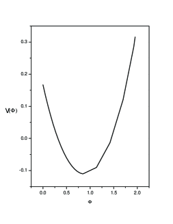
FIG. 1.: This graph shows the integrated scalar field potential obtained for a non-singular universe in a flat universe. Notice that again the potential has negative values near the origin.

We notice that it seems possible to generate a cousin model, for every model based on a closed geometry, by using negative potentials. In this context, we can also study a model similar to the “Emergent Universe” proposed in [15]. In that reference is assumed that our universe is closed and the authors worked out an example where the universe start in a static Einstein state which evolve towards an expanding phase that leads to inflation. Based on our results in this section it seems probable to construct a similar model in a flat universe but with negative potentials.

IV Quintessence-matter interaction

In the previous section we derived a set of equations for a simple non flat model where a scalar field and matter have an asymptotic constant energy densities ratio $r(t)\equiv\Omega_{m}/\Omega_{\varphi}$.  This model can be easily generalized to the case where a explicit interaction is added between matter and dark energy.

If we consider an explicit interaction, then Eq.(2) and the equation of motion of the fluid become modified by

$$\ddot{\varphi}+3H\dot{\varphi}+V^{\prime}(\varphi)=\zeta,$$ (15)

$$\dot{\rho}_{m}+3H(\rho_{m}+p_{m})=-\zeta\dot{\varphi},$$ (16)

where $\zeta$ specify the interaction, and $\rho_{m}$ and $p_{m}$ are the matter energy and pressure densities. There are many ways to couple these components, for example in [5] Wetterich uses $\zeta=\alpha\rho_{m}$ resembling the coupling between baryons and nucleons in GUT theories and Chimento et al.[6] use $\zeta=3\Pi H/\dot{\varphi}$ where $\Pi$ is certain density dissipative pressure. Another class of interaction is of the type $\zeta=-\Gamma\dot{\varphi}$  where $\Gamma$ is a constant which depends on physical parameters of the particle model. This kind of interaction is known in the theory of reheating where $\Gamma$ is interpreted as the rate of particle decay from the inflaton field to radiation. For simplicity, in the rest of the section we restrict the analysis to a universe with $k=0$.

Let us start the analysis with $\zeta=\alpha\rho_{m}$. The Friedman equation is the same as Eq.(1) with $k=0$ where now $\rho=\rho_{\varphi}+\rho_{m}$. Essentially the key expression to obtain here is the analog of Eq.(4).

From the Friedman equation we obtain

$$\frac{\dot{\rho}_{\varphi}}{\rho_{\varphi}}=2\frac{\dot{H}}{H}-\frac{\dot{r}}{(1+r)}$$ (17)

From Eq.(15) we can calculate the same ratio as

$$\frac{\dot{\rho}_{\varphi}}{\rho_{\varphi}}=-3H(1+\omega(\varphi))+\alpha\dot{\varphi}r$$ (18)

Because we are interested in the asymptotic evolution of the system, and we want to obtain a scalar field potential with the property of tracking behavior, we set $r=r_{0}=$ constant for the rest of the analysis. This assumption enable us to obtain a universe without the coincidence problem. To extract more information from this method we have to assume also the evolution of the matter density. Actually this is what must be done if we want to perform the same analysis in section II with a variable $r(t)$. This is not so tricky because we are looking for asymptotic solutions where we assume the scalar field and the matter density have already reached smooth evolutions. If this assumption is not correct, then can not get consistent solutions. So, let us consider the case where $\rho_{m}\sim t^{-q}$. It immediately implies a temporal evolution for the time derivative of the scalar field, because we have assumed before that $r=r_{0}$, so $\dot{\varphi}\sim t^{-q/2}$. This also affects the evolution of Eq.(16). From this we obtain that $\alpha\dot{\varphi}\sim t^{-1}$, implying $q=2$. Of course we want to obtain a solution of the form similar to Eq.(9), so the previous expression for $\dot{\varphi}$ has to be taken as an ansatz. The final result has to be consistent with this analysis.

Combining Eq.(17) and (18) we obtain the generalization of Eq.(4)

$$1+\omega(\varphi)=\frac{1}{3H}\left[-\frac{2}{3}\frac{\dot{H}}{H}+\frac{r_{0}C}{t}\right].$$ (19)

where $C=\alpha\dot{\varphi}_{0}$. From this relation and by inspection of Eq.(5) is direct to obtain the case where $k\neq 0$. The formulaes for constructing the potential and scalar field are in this case

$$V(t)=\frac{3H^{2}}{8\pi G}\left(1+\frac{1}{3}\frac{\dot{H}}{H^{2}}-\frac{r_{0}C}{6Ht}\right),$$ (20)

and

$$\dot{\varphi}^{2}(t)=\frac{3H^{2}}{8\pi G}\left(-\frac{1}{3}\frac{\dot{H}}{H^{2}}+\frac{r_{0}C}{6Ht}\right).$$ (21)

If we consider a power law evolution, $a(t)=a_{0}t^{n}$, then we find that $H=nt^{-1}$ and $\dot{H}=-nt^{-2}$, so replacing in Eq.(20) and (21) we find

$\displaystyle V(\varphi)=V_{0}\exp(-\lambda\varphi),$

with

$$V_{0} = \frac{1}{8\pi G}\left((3n-1)n+\frac{nr_{0}C}{2}\right),$$

$$\lambda = \sqrt{8\pi G}\left(n(1+\frac{r_{0}C}{2})\right)^{-1/2},$$

and the scalar field evolve as

$\displaystyle\varphi(t)=\sqrt{\frac{n}{8\pi G}\left(1+\frac{r_{0}C}{2}\right)}\ln t,$

consistent with our ansatz. We may think that this method is not so helpful because from the very beginning we have found $\dot{\varphi}\sim t^{-1}$ and also, from the definition of $\rho_{\varphi}$, the relation $V\sim t^{-2}$, leading to an exponential potential. But this is just an ansatz and we need the complete solution to understand all the consequences.

V Non-zero curvature case

In this section we perform the application of the equations derived in section I. Let us assume first a universe without interaction between matter components, $\zeta=0$. As a first example, we study the well known problem of a closed ($k=1$) oscillatory universe, that with a scale factor evolving as $a(t)=a_{0}\sin(\alpha t)$. If a matter component is present we assume that the ratio $r(t)=r_{0}$ is a constant. By introducing the scale factor in the reconstruction equations we find

$$V(\varphi) = \frac{3(1+r_{0})^{-1}}{8\pi G}\times$$ (23)

$$\times\left[\frac{2}{a_{0}^{2}}-\frac{\alpha^{2}}{3}+2\left(\frac{1}{a_{0}^{2}}+\frac{\alpha^{2}}{3}\right)\sinh(\left|\varphi/\varphi_{c}\right|),\right]$$

where we have define

$\displaystyle\varphi_{c}=\sqrt{\frac{1}{4\pi G}\left(\frac{\alpha^{2}-a_{0}^{-2}}{1+r_{0}}\right).}$

The scalar field derivative is

$\displaystyle\dot{\varphi}^{2}(t)=\varphi_{c}^{2}(1+\cot^{2}(\alpha t)).$

A subtle treatment of this equation leads to the $\left|\varphi\right|$ dependence of $V(\varphi)$. After we take the square root, we can define two branches: those where $\dot{\varphi}>0$, and $\dot{\varphi}<0$. Taking care of this conditions we found that

$\displaystyle\sinh\alpha\left|\frac{\varphi}{\varphi_{c}}\right|=\cot(\alpha t).$

The potential (23) looks like Fig. 2.

FIG. 2.: This graph shows a typical scalar field potential used in a closed inflationary model. The scale is arbitrary.

Of course, this potential can also drive chaotic inflation. The Emergent Universe [15] is a special case of a system where we impose a solution like $a(t)=A+B\exp(\alpha t)$.

VI Results

The method presented in this paper looks extremely important theoretically for the study of model building in cosmology. Although it is not the first paper on this subject we have generalized the recipe to construct scalar field potential for arbitrary curvature and also with an explicit interaction between matter and the scalar field.

The interaction between matter components give us the possibility to address the coincidence problem without appealing to any other tracker property. In fact, in the case of tachyons, the tracker evolution does not work but is possible to get a similar tracking behavior by using an explicit interaction.

By considering non-zero curvature lead us to many different models where is possible to integrate the evolution. In particular, during the last years there have been some controversy about considering inflation in a closed geometry [11]. In this paper we shows a explicit model where inflation can be obtained followed by a oscillating reheating phase. The Emergent Universe proposed in [15] is a special case of a system where we impose a solution like $a(t)=A+B\exp(\alpha t)$.

The applications are multiple; inflationary building models and also the more recently dark energy problem or quintessence. Although is always possible to use the construction equations found in this paper, we stress that in general we can not extract a explicit shape of the potential. Probably the main interest in this kind of construction technic is the possibility to extract some information about the shape of the potential in certain ranges and then look for those features in well motivated theoretical models.

VII Acknowledgments

The authors would like to thank Ioav Waga for useful conversations and comments. This work has been supported by projects FONDECYT grant 3010017 (VHC) and 1030469 (SdC). Also, it was partially supported by UCV grant No. 123.764/03.

REFERENCES

- [1] C.L. Bennett et al., arXiv: astro-ph/0302207.
- [2] G. Dvali, G. Gabadadze and M. Shifman, Phys. Rev. D 67 044020 (2003); G. Dvali and M.S. Turner, astro-ph/0301510; S.M. Carroll, V. Duvvuri, M. Trodden, M.S. Turner, astro-ph/0306438; K. Freese, M. Lewis, Phys. Lett. B540, 1 (2002).
- [3] C. Wetterich, Nucl. Phys. B 302, 645 (1988); P.J.E. Peebles and Ratra, Ap. J. 325, L17 (1988).
- [4] I. Zlatev, L. Wang, and P.J. Steinhardt, Phys. Rev. Lett. 82, 896 (1998); P.J. Steinhardt, L. Wang and I. Zlatev, Phys. Rev. D 59,123504 (1999); A.R. Liddle and R.J. Scherrer, Phys. Rev. D 59,023509 (1999).
- [5] C. Wetterich, Astron.Astrophys. 301, 321 (1995).
- [6] L. Amendola, Phys. Rev. D 62,043511 (2000); L.P.Chimento, A.S. Jakubi, D. Pavón and W. Zimdahl, arXiv: astro-ph/0303145; G.R. Farrar and P.J.E. Peebles, astro-ph/0307316.
- [7] T. Padmanabhan, Phys. Rev. D 66, 021301 (2002), arXiv: hep-th/0204150; see also section 4.3 of T. Padmanabhan, Theoretical Astrophysics, Vol III: Galaxies and Cosmology, Cambridge U. Press, Cambridge (2002).
- [8] G.F.R. Ellis and M.S. Madsen, Class. Quant. Grav. 8, 667 (1991).
- [9] G.F.R. Ellis, J. Murugan, and C.G. Tsagas, gr-qc/0307112.
- [10] S.A. Pavluchenko, astro-ph/0304354.
- [11] G. Efstathiou, MNRAS 343, L95 (2003); A. Linde, astro-ph/0303245; J.P. Uzan, U. Kirchner and G.F. Ellis, astro-ph/0302597; A. Lasenby and C. Doran, astro-ph/0307311.
- [12] G. Felder, A. Frolov, L. Kofman and A. Linde, Phys.Rev. D 66 023507 (2002), arXiv: hep-ph/0202017; I.P.C. Heard and D. Wands, Class.Quant.Grav.19 5435 (2002), arXiv: gr-qc/0206085.
- [13] J. Khoury, B. Ovrut, N. Seiberg, P. Steinhardt and N. Turok, Phys. Rev. D 65, 086007 (2002).
- [14] V.H. Cardenas and J. Saavedra, in preparation.
- [15] G.F.R. Ellis and M.S. Madsen, arXiv: gr-qc/0211082; G.F.R. Ellis, J. Murugan and C.G. Tsagas, arXiv: gr-qc/0307112.