A Study of QSO Evolution in the X-ray Band with the Aid of Gravitational Lensing

Abstract

We present results from a mini-survey of relatively high redshift ($1.7<z<4$) gravitationally lensed radio-quiet quasars observed with the Chandra X-ray Observatory and with XMM-Newton. The lensing magnification effect allows us to search for changes in quasar spectroscopic and flux variability properties with redshift over three orders of magnitude in intrinsic X-ray luminosity. It extends the study of quasar properties to unlensed X-ray flux levels as low as a few times $10^{-15}$erg cm^-2 s^-1 in the observed 0.4–8 keV band. For the first time, these observations of lensed quasars have provided medium to high signal-to-noise ratio X-ray spectra of a sample of relatively high-redshift and low X-ray luminosity quasars. We find a possible correlation between the X-ray powerlaw photon index and X-ray luminosity of the gravitationally lensed radio-quiet quasar sample. The X-ray spectral slope steepens as the X-ray luminosity increases. This correlation is still significant when we combine our data with other samples of radio-quiet quasars with $z>1.5$, especially in the low luminosity range between $10^{43}$–$10^{45.5}~{}\hbox{erg~{}s${}^{-1}$}$. This result is surprising considering that such a correlation is not found for quasars with redshifts below 1.5. We suggest that this correlation can be understood in the context of the hot-corona model for X-ray emission from quasar accretion disks, under the hypothesis that the quasars in our sample accrete very close to their Eddington limits and the observed luminosity range is set by the range of black hole masses (this hypothesis is consistent with recent predictions of semi-analytic models for quasar evolution). The upper limits of X-ray variability of our relatively high redshift sample of lensed quasars are consistent with the known correlation between variability and luminosity observed in Seyfert 1s when this correlation is extrapolated to the larger luminosities of our sample.

1 Introduction

It is important to extend the study of quasars to high redshifts in order to understand the evolution of quasars and their environments. One of the main results of recent studies of quasar evolution is that the quasar luminosity function evolves strongly with redshift. (e.g. Boyle et al. 1987). Many studies of quasar evolution are aimed at explaining this luminosity evolution. The X-ray band probes the innermost regions of the central engine of the Active Galactic Nuclei (AGN). The study of AGN in X-rays may possibly answer the question of whether there is an evolution in their central engines and how this is related to the evolution of the quasar luminosity function. The observed X-ray continuum emission of AGN is generally modeled by a power law of the form $N(E)=N_{0}(E/E_{0})^{-\Gamma}$ where $N(E)$ is the number of photons per unit energy interval. Extensive studies of AGN during the past decade indicate that this power-law component is produced by Compton scattering of soft photons by hot electrons in a corona (e.g., Haardt & Maraschi, 1993; Haardt, Maraschi, & Ghisellini, 1994). The study of this power-law component, its correlations with other AGN parameters, and its evolution reveals important information on the accretion process of the central object. The X-ray photon indices of low-redshift radio-quiet quasars are measured to have mean values of $\sim$2.6–2.7 in the ROSAT soft X-ray band (Laor et al., 1997; Yuan et al., 1998) and $\sim$1.9–2.0 for the ASCA hard X-ray band (George et al., 2000; Reeves & Turner, 2000), and are correlated with the $\rm{H}\beta$ FWHM (Reeves & Turner, 2000). There is no strong evidence that the X-ray power-law index evolves with redshift or correlates with X-ray luminosity to date (George et al., 2000; Reeves & Turner, 2000). Another important parameter that describes the broad band spectral shape of quasars is the optical-to-X-ray spectral index, quantified as $\alpha_{\rm ox}=\log(f_{\rm{2keV}}/f_{2500{\AA}})/\log(\nu_{\rm{2keV}}/\nu_{2500~{}\AA})$, where $f_{{\rm 2keV}}$ and $f_{2500~{}\AA}$ are the flux densities at 2 keV and 2500 Å in the quasar rest-frame, respectively. Recently, several studies have provided estimates of $\alpha_{\rm ox}$ for very high redshift ($z>4$) quasars (Vignali, Brandt, & Schneider, 2003; Vignali et al., 2003a, b; Bechtold et al., 2003). Vignali, Brandt, & Schneider (2003); Vignali et al. (2003a, b) found that $\alpha_{\rm ox}$ is mainly dependent on the ultra-violet luminosity while Bechtold et al. (2003) found that $\alpha_{\rm ox}$ primarily evolves with redshift. In addition to spectral studies, variability studies of Seyfert galaxies show that the variability amplitude (excess variance) is anti-correlated with X-ray luminosity (Nandra et al., 1997; Leighly, 1999). Variability studies have been extended to quasars by several groups (George et al., 2000; Almaini et al., 2000; Manners, Almaini, & Lawrence, 2002). Low redshift quasars ($z<2$) are found to have an excess variance consistent with the luminosity relation found in Seyfert 1s and there is a possible upturn of X-ray variability for high redshift quasars with $z>2$ (Almaini et al., 2000; Manners, Almaini, & Lawrence, 2002).

It is also important to compare the properties of quasars near the peak of their comoving number density, thought to have occurred at $z\sim 2$, with low redshift quasars. This comparison may provide clues as to what caused the dramatic decay of the quasar number density as the Universe expanded.

Most of the observational and analysis techniques employed to date to study the evolution and emission mechanism of faint, high-redshift quasars are based on either summing the individual spectra of many faint X-ray sources taken from a large and complete sample or obtaining deep X-ray observations of a few quasars. Although these techniques may yield important constraints on the average properties of high redshift quasars they each have significant limitations.

Gravitational lensing provides an additional method for studying high-redshift quasars. The extra flux magnification, from a few to $\sim$100, provided by the lensing effect enables us to obtain high signal-to-noise ratio (S/N) spectra and light-curves of distant quasars with less observing time and allows us to search for changes in quasar spectroscopic properties and X-ray flux variability over three orders of magnitude in intrinsic X-ray luminosity. With the aid of lensing, we can probe lower flux levels than other flux limited samples with similar instruments and exposures. This could be an important factor because the X-ray properties of high-redshift, low-luminosity quasars could be different from those of other quasars and by studying them we could possibly obtain information about the evolution of quasars.

Similar lensing studies have also been performed in the sub-millimeter and CO bands (Barvainis & Ivison, 2002; Barvainis, Alloin, & Bremer, 2002), which suggested that gravitational lensing could be an efficient method for studying various properties of high-redshift quasars. Here we present the results of an X-ray mini-survey of relatively high redshift gravitationally lensed radio-quiet quasars. We chose only the radio-quiet quasars in our sample because the powerful relativistic jets in the radio-loud quasars will introduce additional complication when modeling the continuum X-ray emission from the accretion disc.

We use a $H_{0}$ = 50 km s^-1 Mpc^-1 and $q_{0}=0.5$ cosmology throughout the paper.

2 Observations and Data Reduction

Our mini-survey contains eleven gravitationally-lensed, radio-quiet quasars with redshifts ranging between 1.695 and 3.911. Five of them contain Broad Absorption Lines (BALs) or mini-BALs in their rest-frame ultraviolet spectra. Most of the lensed quasars of our sample were observed with the Advanced CCD Imaging Spectrometer (ACIS; Garmire et al. 2003) onboard Chandra as part of a Guaranteed Time Observing program (Principal Investigator: G. Garmire). The data for two of the them were obtained through the public Chandra archive. Several of them were observed twice. Three of the lensed quasars were also observed with XMM-Newton. Table 1 presents a log of observations, including redshifts, Galactic column densities, and exposure times. Each observation was performed continuously with no interruptions.

All of the sources observed with Chandra were placed near the aim point of the ACIS-S array, which is on the back-illuminated S3 chip. All of the data were taken in FAINT or VERY FAINT mode. The Chandra data were reduced with the CIAO 2.3 software tools provided by the Chandra X-Ray Center (CXC) following the standard threads on the CXC website. Only photons with standard ASCA grades of 0, 2, 3, 4, 6 were used in the analysis. We used events in the 0.4–8 keV energy range in the spectral analysis and events in the 0.2–10 keV range for the variability studies. The source events were extracted from circles with radii ranging from 3^′′ to 5^′′ depending on the separations of the lensed images of each quasar. The circles included all of the lensed images. Background events were extracted from annuli with inner and outer radii of 10^′′ and 30^′′, respectively, centered on the sources. We adjusted the inner and outer radii of the background subtraction annuli in some cases to avoid other sources in the field. The background contributes an insignificant amount to the count rate in a source region, even during a background flare. The average exposure time for the Chandra observations was about 25 ks. The detected source count rates ranged between 0.003–0.08 $\rm{s^{-1}}$.

Three targets were observed with the European Photon Imaging Camera PN and MOS detectors (Strüder et al., 2001; Turner et al., 2001) onboard XMM-Newton. The XMM-Newton data were analyzed with the standard analysis software, SAS 5.3. The tasks epchain and emchain from SAS were used to reduce the PN and MOS data and photons of patterns $\leq 4$ and $\leq 12$ were selected from the PN and MOS data, respectively. The XMM-Newton data are affected more than the Chandra data by background flares because the Point Spread Function of XMM-Newton is significantly larger than that of Chandra-ACIS. Several strong background flares occurred during the XMM-Newton observations. These flares are filtered out in the spetral analysis.

3 Spectral Analysis

3.1 Power-law Continuum

We performed spectral fitting in order to obtain the power-law indices of the X-ray continuum emission components of the quasars in our sample. The photon indices that we measured were in the observed 0.4–8 keV energy range. We used the Chandra data for all of the lensed quasars in the spectral analysis except PG 1115+080, where we used the XMM-Newton data. RX J0911.4+0551 and APM 08279+5255 were also observed with XMM-Newton. We did not use these data, however, because there were large amplitude and long duration background flares in the XMM-Newton observations. The background flare in the XMM-Newton observation of RX J0911.4+0551 almost spans the entire observation. The background flare in the XMM-Newton observation of APM 08279+5255 occurs during the last $\sim 20$ ks of the observation. We filtered the background flare time from this observation and performed a spectral analysis to compare with our Chandra results. For our later correlation analysis, we used the Chandra data of APM 08279+5255 to avoid the possible complication from the cross calibration between Chandra and XMM-Newton instruments. For those sources observed twice with Chandra, we performed simultaneous fits to the spectra extracted from the two observations except in the case of APM 08279+5255, where we used only the second observation because it was much longer than the first one.

We extracted spectra for each quasar using the CIAO tool psextract. We extracted events from all of the lensed images for each source except for the case of H 1413+117. A possible microlensing event in H 1413+117 appears to amplify and distort the spectrum of image A only and thus affects the spectral slope greatly (Chartas et al., 2003). In this case, we extracted the spectrum of the microlensed image A and the spectrum of the other three images separately. A microlensing event is also detected in Q 2237+0305. However, the spectral shape of the microlensed image A of Q 2237+0305 is not significantly affected by the microlensing event (Dai et al., 2003).

Spectral fitting was performed with XSPEC V11.2 (Arnaud, 1996). There are typically several hundreds (180–6000) detected source events in the spectra of the target quasars, except for the spectrum of HE 2149$-$2745 which has only 23 detected events. The moderate S/N of our spectra allows us to fit each of them individually using relatively complex models. Thus we can constrain the underlying power-law slopes more accurately than in previous studies of unlensed quasars of similar redshift. The models we used are listed in Column 3 of Table 2. All spectral models included an underlying power-law model modified by Galactic absorption. The Galactic absorbing columns were obtained from Dickey & Lockman (1990).

To account for the recently observed quantum efficiency decay of ACIS, possibly caused by molecular contamination of the ACIS filters, we have applied a time-dependent correction to the ACIS quantum efficiency implemented in the XSPEC model ACISABS1.1. If the source was a BALQSO with a medium S/N spectrum, we added a neutral absorption component at the redshift of the source. For high S/N BALQSO spectra such as PG 1115+080 and APM 08279+5255 we used the absori model in XSPEC to model the intrinsic absorption component as an ionized absorber (Chartas et al., 2002; Chartas, Brandt, & Gallagher, 2003). We added a neutral absorption component at the redshift of the lens for Q 2237+0305 (Dai et al., 2003). For some of the spectra containing emission or absorption line features, we added Gaussian line components to model them accordingly. The spectra of the quasars are displayed in Figures 1. The spectral fitting results are given in Table 2. In Table 2, we also list the observed 0.4–8 keV fluxes and rest-frame 0.2–2 keV and 2-10 keV luminosities for the lensed quasars in the sample not corrected for the lensing magnification. The unlensed luminosities are calculated in $\S$4. We have corrected for the various absorption components when calculating X-ray luminosities. These absorption components include Galactic absorption, absorption in the lensing galaxy, intrinsic absorption, and the ACIS contamination.

The mean photon index of the radio-quiet quasars in our sample is $1.78\pm 0.06$ with a dispersion of $0.27\pm 0.08$ and the median photon index of the radio-quiet quasars in our sample is 1.86.

3.2 $\alpha_{\rm ox}$

We calculated the optical-to-X-ray power-law slope, $\alpha_{\rm ox}$, for the quasars in our sample. The differential magnification between the optical and X-ray band is insignificant because both of the source regions are estimated to be much smaller than the Einstein radius. The rest-frame 2 keV flux densities were calculated from the best-fit models to the spectra of the quasars. The redshifts of our sample range from 1.7 to 4, thus the rest-frame 2 keV energy falls in the 0.4–0.74 keV observed-frame energy range. We removed all of the absorption components including the intrinsic ones for the BALQSOs when calculating the rest-frame 2 keV flux densities in order to study the properties of the intrinsic continuum. The rest-frame 2500 Å fluxes were obtained from the published optical data in the literature and from current ongoing programs such as the CfA-Arizona Space Telescope LEns Survey (CASTLES) and the Optical Gravitational Lensing Experiment (OGLE). We first converted the optical magnitudes to flux densities at the effective wavelengths of the filters, then extrapolated them to the rest-frame 2500 Å flux densities. We used the standard relations between magnitudes and flux densities for the V and R bands. For the F814W magnitudes obtained with the HST WFPC2, we used the relation from Holtzman et al. (1995) to convert between magnitudes and flux densities. We used $f_{\nu}\propto\nu^{-0.7}$ in the extrapolation. Typical quasar optical spectral indices are in the -0.5 to -0.9 range (Schneider et al., 2001). We chose the optical magnitudes from the bands closest to the redshifted 2500 Å wavelength to reduce the error in the extrapolation. We corrected the Galactic extinction based on Schlegel, Finkbeiner, & Davis (1998). The extinction induced by the dust from the lensing galaxies is not significant except for Q 2237+0305, which is lensed by the central bulge of the galaxy. We corrected it according to the appendix of Agol, Jones, & Blaes (2000). The $\alpha_{\rm ox}$ values are listed in Table 3. The listed error-bars of $\alpha_{\rm ox}$ are at the $1\sigma$ level and account for the uncertainties in the X-ray spectral slope and normalization, the conversion from optical magnitude to flux density and the extrapolation of the optical/UV spectrum. We note that a source may have varied between the optical and X-ray observations thus leading to systematic errors in our estimates of $\alpha_{\rm ox}$. For the range of $\alpha_{\rm ox}$ in our sample, a change of optical flux by a factor of two will lead to a change of $\Delta$$\alpha_{\rm ox}$$\sim 0.1$. The rest-frame 2 keV and 2500Å flux densities and rest-frame 2500Å luminosity densities are also listed in Table 3. These values are corrected for lensing magnification as we discuss further in $\S$4. In conclusion we find that the mean $\alpha_{\rm ox}$ value for all the quasars in our sample is $-1.70\pm 0.02$ ($-1.66\pm 0.02$ without HE 2149$-$2745 which has only 23 X-ray events) with a dispersion of $0.20\pm 0.03$.

4 Magnification and Intrinsic X-ray Luminosities

We estimated the magnification for each of the lensed systems in order to obtain the unlensed X-ray luminosities of the quasars. We first searched in the literature for magnifications of well-modeled systems. However, not all of the systems in our sample have been previously modeled in detail and for some cases the magnification values are not included in the published analysis. We modeled these systems with the gravlens 1.04 software tool developed by C. Keeton (Keeton, 2001a, b). We used a singular isothermal elliptical (SIE) mass profile with external shear in most cases, and took into account optical image positions and flux ratios obtained from the CASTLES survey. We assumed a 20% error-bar for the flux ratios to account for uncertainties from microlensing or differences between optical and X-ray flux ratios. Our modeling results are listed in Table 4. We compared the magnification values that we obtained with those published in Barvainis & Ivison (2002) and found them to be in good agreement. We note that the magnification values obtained may have large systematic errors because the SIE model adopted in this analysis may not be suitable for all the systems. For example, in PG 1115+080, a set of different mass potentials are used in the modeling of the magnification in Impey et al. (1998). A magnification range of 20–46 was obtained for this system. Based on this example, we adopt a factor of two as a typical systematic uncertainty in the magnification. In $\S$6.1 we investigate how this systematic uncertainty could affect for our conclusions via Monte Carlo simulations.

5 Variability Analysis

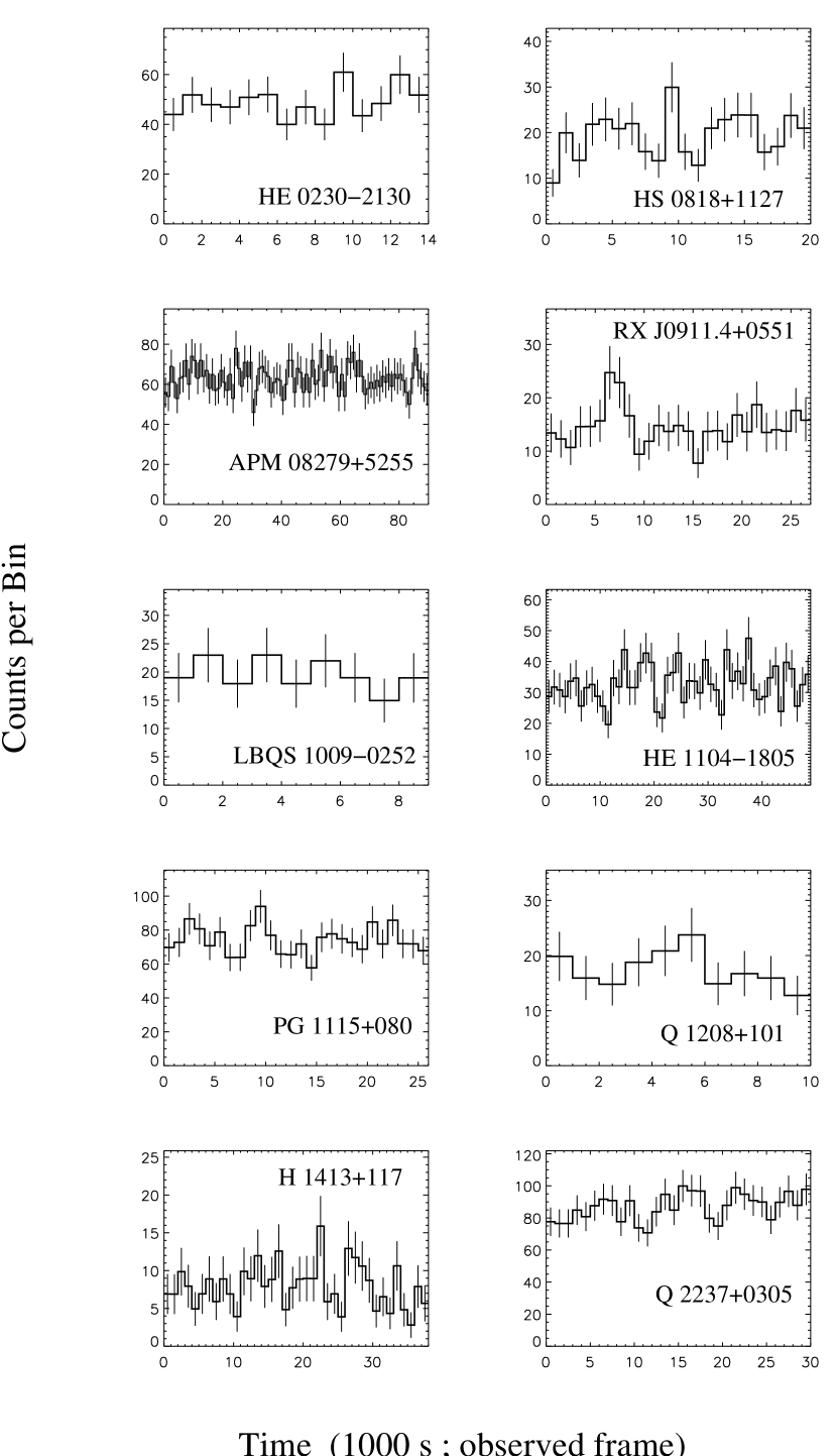
Figure 2: Light-curves of gravitationally lensed radio-quiet quasars observed with Chandra. The light-curves are binned with a bin size of 1000 s in the observed-frame.

The light-curves for the Chandra observations of the lensed quasars of our sample are displayed in Figure 2 binned with a bin size of 1000 s (observed-frame). We show the light-curves of the longer Chandra exposure if two Chandra observations of the same target are available. We excluded HE 2149$-$2745 in our timing analysis because of its low S/N (only 23 events).

To estimate the relative variability of the light-curves, we used the normalized excess variance (Nandra et al., 1997; Turner et al., 1999; Edelson et al., 2002) defined as

$$\sigma^{2}_{\rm rms}=\frac{1}{N\mu^{2}}\sum_{i=1}^{N}[(X_{i}-\mu)^{2}-\sigma_{i}^{2}]$$ (1)

where $N$ is the number of bins in the light-curve, $X_{i}$ are the count rates per bin with error $\sigma_{i}$, and $\mu$ is the mean count rate. The error on $\sigma^{2}_{\rm rms}$ is given by $S_{D}/[\mu^{2}(N)^{1/2}]$, where

$$S_{D}^{2}=\frac{1}{N-1}\sum_{i=1}^{N}\{[(X_{i}-\mu)^{2}-\sigma_{i}^{2}]-\sigma^{2}_{\rm rms}\mu^{2}\}^{2}$$ (2)

This method normalizes the variability amplitude to the flux, thus is less biased towards the low flux light-curves. It is better to apply this method to a sample of light-curves of similar lengths to avoid possible bias. For example, it would be easier to detect long time-scale variability from a light-curve with a long duration. In addition, the bin sizes should be similar in order to compare variability on similar time-scales. High S/N light-curves are needed for this analysis as the variability could be easily dominated by noise in the low S/N light-curves. This excess variance method also has some limitations. One of them is that it is not very sensitive to short flares of moderate amplitude. The excess variance values for Chandra light-curves with three different bin sizes are listed in Table 5. We also calculated the excess variance for the three sources observed with XMM-Newton and the results are listed in Table 6. The background was subtracted in the calculation. Overall, the error-bars on the excess variance are quite large and in some cases, the values are negative. Therefore, for most quasars we can really only obtain an upper limit on the value of the excess variance.

6 Results and Discussion

6.1 Luminosity and Spectral Index

The unlensed 0.2–2 keV and 2–10 keV X-ray luminosities of the lensed quasars in our mini-survey range from $10^{43}$ to $10^{46}$ erg s^-1. The mean spectral index of our sample, 1.78, is consistent with the value of 1.84 from the recent study of very high redshift quasars (Vignali et al., 2003b) and the value of 1.89 from the radio-quiet ASCA sample (Reeves & Turner, 2000), especially when one considers the large dispersion of spectral indices in these studies and our small sample size.

We plot the rest-frame 0.2–2 keV and 2–10 keV X-ray luminosity against redshift in Figure 3(a), and the photon indices vs. redshift, 0.2–2 keV luminosity, and 2–10 keV luminosity in Figures 3(b), (c), and (d), respectively. Figures  3(c) and (d) show a correlation between the spectral indices of our sample of lensed quasars and their X-ray luminosities. We tested the significance of this correlation using the Spearman’s rank correlation method. We obtained a rank correlation coefficient of 0.94 significant at the greater than 99.997% confidence level for the correlation between photon index and 0.2–2 keV luminosity and a coefficient of 0.71 significant at the 98.6% confidence level for the correlation between photon index and 2–10 keV luminosity. We note that the measured rest-frame 0.2–2 keV luminosity for high redshift quasars obtained from Chandra and XMM-Newton data is less accurate than the rest-frame 2–10 keV luminosity because it depends on extrapolation and suffers from the uncertainty in the absorbing columns towards the quasars. We adopt a significance at the 98.6% confidence level for this correlation, evaluated with the 2-10 keV luminosities. We also tested for a possible correlation between X-ray luminosity and redshift and between photon index and redshift and found none.

The correlation between the photon index and X-ray luminosity was a surprising result. Therefore, we tested if this correlation is driven by certain data points. Excluding one of our data points at a time and performing the Spearman’s rank correlation between $\Gamma$ and the 0.2–2 keV luminosity to the rest of the data set, we find a strong correlation with a significance level greater than 99.98% each time. We performed a similar analysis with the 2–10 keV luminosity, and the correlation is significant at the greater than 95% confidence level each time. This indicates that the correlation is not driven by any particular data point. We further performed correlation tests by excluding data points with errors in $\Gamma$ larger than 0.20. Two data points are excluded and the rest of the data points still show a correlation significant at the greater than 99.98% confidence level. The significance is at the 92% confidence level when 2–10 keV luminosities are used. We also tested if there is a bias from different flux levels in our sample such that quasars with low fluxes have a systematically flatter slope because of measurement errors. In principle, this should not be a problem for the sample in this paper because some low luminosity quasars have high S/N spectra as a result of the gravitational lensing effect. To test this, we simulated spectra with the same photon index ($\Gamma=2$) but with a wide range of S/N and then fitted them with the same models within XSPEC. We found that for low S/N spectra, when the total number of photons is less than $\sim$200, the measured $\Gamma$ could possibly be flatter by $\sim 0.1$. This would affect three of our data points: HE 2149$-$2745, LBQS 1009$-$0252, and Q 1208+101 with (one low-luminosity and two high-luminosity quasars). We tested this effect by increasing the photon index by 0.1 for these three quasars and performed the correlation test again and found the correlations between $\Gamma$ and 0.2–2 keV (2–10 keV) luminosities are significant at the 99.99% (98.7%) confidence levels, respectively.

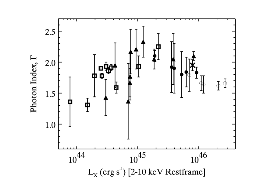
Figure 4: $\Gamma$–$L_{X}$ (2–10 keV rest-frame) diagram for high redshift quasars ($z>1.5$). The data shown as filled triangles are from Page et al. (2003). The data shown as filled circles are from Reeves & Turner (2000). The data shown as crosses are from George et al. (2000). The data shown as open circles are from Vignali et al. (1999). The data shown as open squares are from our own sample of lensed quasars.

A $\Gamma$–${L_{X}}$ correlation has been previously searched for in other samples of radio-quiet quasars. Reeves et al. (1997) reported first a possible correlation between $\Gamma$ and luminosity with nine radio-quiet quasars observed with ASCA. However, this correlation was later not found in the study of a larger sample of 27 radio-quiet quasars observed with ASCA (including the original nine) by Reeves & Turner (2000). George et al. (2000) also searched for a correlation between $\Gamma$ and luminosity in another sample of radio-quiet quasars observed with ASCA and did not find one. However, the quasars in our sample all have relatively high redshifts $1.7<z<4$ compared to the redshifts of quasars incorporated in previous studies of the $\Gamma$–$L_{X}$ correlation. There is only one out of 26 quasars with $z>1.5$ in the sample of George et al. (2000), and there are six out of 27 quasars with $z>1.5$ in the sample of Reeves & Turner (2000) and most of them have large errors on $\Gamma$. In addition, the high redshift quasars in the sample of George et al. (2000) and Reeves & Turner (2000) have high luminosities and span a small luminosity range of $10^{45}$–$10^{46}~{}\hbox{erg~{}s${}^{-1}$}$. The sample of lensed quasars in this paper have lower luminosities and span a larger luminosity range of $10^{43}$–$10^{45}~{}\hbox{erg~{}s${}^{-1}$}$. Recently, Page et al. (2003) presented another sample of quasars observed with XMM-Newton which contains several high redshift, low-$L_{X}$ quasars. We plotted the $\Gamma$–$L_{X}$ diagram for quasars of $z>1.5$ from the sample of Page et al. (2003), Reeves & Turner (2000), George et al. (2000), and Vignali et al. (1999) in Figure 4. We excluded one data point from Page et al. (2003) with a large measurement error on $\Gamma$. We also excluded PHL 5200 from Reeves & Turner (2000) in our analysis because new XMM-Newton observations of the object showed that most of the X-rays originate from a nearby radio source (Brinkmann, Ferrero, & Gliozzi, 2002). We corrected the X-ray luminosity of HE 1104$-$1805 reported in Reeves & Turner (2000) to account for the gravitational lensing magnification of about 12 based on our analysis presented in $\S$4. We used rest-frame 2-10 keV luminosities in order to be consistent with the previous analysis. Most of the data from Page et al. (2003) are consistent with the $\Gamma$–$L_{X}$ correlation found in our sample of lensed quasars, especially in the low $L_{X}$ range between $10^{43.5}$–$10^{45.5}~{}\hbox{erg~{}s${}^{-1}$}$. On the high luminosity end ($L_{X}>3\times 10^{45}~{}\hbox{erg~{}s${}^{-1}$}$) of high redshift quasars ($z>1.5$), the $\Gamma$ dependence on $L_{X}$ seems to flatten out or even has an anti-correlation pattern. We performed the Spearman’s rank correlation test to all of the ($z>1.5$) quasars and did not find a correlation between $\Gamma$ and 2–10 keV luminosity. We separated the quasars in two groups with luminosities below and above $3\times 10^{45}~{}\hbox{erg~{}s${}^{-1}$}$ and performed the rank correlation again to each group. The low luminosity quasars show a strong correlation between $\Gamma$ and 2–10 keV luminosity at the 99.97% confidence level and the high luminosity quasars show an anti-correlation between $\Gamma$ and 2–10 keV luminosity at the 98.9% confidence level.

We performed a Monte-Carlo simulation to test how much the $\Gamma$–$L_{X}$ correlation is affected by the uncertainty of the magnification factors of our lensed quasars. We used the combined data sets from the lensed sample and from the quasars of Page et al. (2003) with $z>1.5$, which show a strong $\Gamma$–$L_{X}$ correlation. We assumed a systematic uncertainty on the magnification of a factor of two (see discussion in $\S$4) and simulated 10,000 data sets with $L_{X}$ perturbed from its measured value randomly, within the range of this error-bar. We fixed the data points from Page et al. (2003) at their original values. We performed the Spearman’s correlation test between $\Gamma$ and 2–10 keV luminosity on the simulated data sets and found that the $\Gamma$–$L_{X}$ correlation in each simulated data set is at least significant at the 98.6% confidence level for 10,000 simulations and 9,888 of them have $\Gamma$–$L_{X}$ correlations significant at the greater than 99.5% confidence level. Therefore, it is unlikely that this correlation is driven by the uncertainties in the magnification factors.

Possible errors in magnification factors, the small number of quasars in the present sample combined with the medium S/N of several of the observations may have led to an unaccounted systematic effect. Additional observations of $z\sim 2$ lensed quasars with better S/N and a more detailed modeling of all the lenses in our sample will help confirm this result. Although the $\Gamma$–$L_{X}$ correlation found in this paper could be a result of selection effect, we discuss possible interpretations of this correlation below.

Previous studies did not find any correlation between $\Gamma$ and $L_{X}$ in low-redshift quasars and Seyfert 1s. Recently, several X-ray monitoring programs of Seyfert galaxies have indicated a correlation between X-ray spectral index and 2–10 keV X-ray flux (Chiang et al., 2000; Petrucci et al., 2000; Vaughan & Edelson, 2001). The spectra of these Seyfert galaxies steepen as the X-ray flux increases. Vaughan & Edelson (2001) suggested that variations of several properties of the X-ray emitting corona (e.g., electron temperature, optical depth, size) with the X-ray flux may explain this $\Gamma$ vs. X-ray-flux relation. Similarly, a $\Gamma$ vs. X-ray-flux relation also exists in some Seyfert 2 and radio-loud objects (Georgantopoulos & Papadakis, 2001; Zdziarski & Grandi, 2001; Gliozzi, Sambruna, & Eracleous, 2003). These observations indicate that although the $\Gamma$–$L_{X}$ relation does not apply to a sample of low-redshift quasars and Seyferts, this relation applies to individual objects. In contrast to the low-redshift quasars, the $\Gamma$–$L_{X}$ dependence found at high redshift, especially in high-redshift and low-$L_{X}$ quasars indicates that these quasars may represent a distinct sub-population of quasars. It is possible that the properties of the X-ray emitting coronae of the high-redshift quasars are more homogeneous than those in the low-redshift quasars.

6.2 Possible Interpretations of the Correlation Between the X-Ray Luminosity and Spectral Index

We explore two possible interpretations of the correlation between the spectral index and the X-ray luminosity in the context of the model of Haardt & Maraschi (1993) and Haardt, Maraschi, & Ghisellini (1994). Our first hypothesis is that there is a narrow range (of order a few) of accreting black hole masses at high redshift while the observed range of observed X-ray luminosities (spanning aproximately two orders of magnitude) is caused by a large range in the accretion rate, i.e., a wide range of Eddington ratios (the ratio of the accretion rate to the Eddington rate). Our second hypothesis is that the opposite is true, namely that the range of accreting black hole masses at high redshift is large (spanning approximately two orders of magnitude), while the Eddington rate is fairly constant and close to unity (i.e., the accretion rate is always fairly close to the Eddington limit, regardless of the mass).

In the model of Haardt & Maraschi (1993) and Haardt, Maraschi, & Ghisellini (1994) the inner accretion disk is sandwiched by a hot, tenuous, possibly patchy corona which emits the hard X-ray photons. The corona cools by inverse Compton scattering of soft photons ($E\lower 2.0pt\hbox{$\;\scriptscriptstyle\buildrel<\over{\sim}\;$}100$ eV) from the underlying disk, which results in the hard X-ray photons that we observe. Haardt, Maraschi, & Ghisellini (1997) explored how the model predictions change for a wide range of the system parameters, namely the optical depth and temperature of the corona and the temperature of the (assumed) black-body spectrum of seed photons. In particular, Haardt, Maraschi, & Ghisellini (1997) found that the 2–10 keV spectral index is nearly proportional to the optical depth in the hot corona and also decreases as the temperature of seed soft-photon spectrum increases. Moreover, in the case of a “compact” corona, i.e., one in which pair production is high enough that the Compton scattering optical depth is dominated by electron-positron pairs, the 2–10 keV spectral index is nearly proportional to the log of the 2–10 keV luminosity, just as we have found observationally.

In our first hypothesis the observed range of luminosities is set by the range of accretion rates, with the black hole mass being nearly constant. In this context the observed correlation might be explained if the optical depth in the hot corona is somehow related to the accretion rate; for example, the density of the corona could increase with accretion rate and so would the optical depth. There is a competing effect, however: as the accretion rate decreases so does the temperature of the underlying thin disk, which provides the seed photons, with the result that the spectral index of the emerging X-ray spectrum increases.

In our second hypothesis, the accretion rate for all objects is very close to the Eddington limit, while the observed range in luminosity is set by a range in black hole masses. In the context of this hypothesis, and under the assumption that the optical depth of the corona is dominated by electron-positron pairs, Haardt, Maraschi, & Ghisellini (1997) predict a correlation between the 2–10 keV spectral index and luminosity just like the one we observe. The optical depth in this case depends only on the “compactness” of the corona, which can be expressed as $\ell_{c}\sim 10^{4}(h/r^{2})(L_{X}/L_{Edd})$ (Haardt & Maraschi, 1993), where $L_{X}/L_{Edd}$ is the ratio of the X-ray luminosity to the Eddington luminosity (roughly proportional to the Eddington ratio) and $h$ and $r$ are the vertical and radial extent of the corona in units of the Schwartzschild radius. Thus, in this scenario, the spectral index could increase if the compactness of the corona increases with black hole mass (See equation 16 of Haardt & Maraschi (1993)), with the consequence that the emerging 2-10 keV luminosity increases as well. Moreover, as the optical depth reaches unity, the spectral index reaches its maximum value and begins to decline for larger optical depths. This feature may explain the turnover that we observe in the spectral index $vs$ luminosity plot of Figure 4. We therefore favor this interpretation over the previous one. This interpretation is also appealing because it is consistent with the predictions of semi-analytic models of Kauffmann & Haehnelt (2000) for the cosmological evolution of supermassive black holes and their fueling rates. In particular, these authors predict that at redshifts between 1.5 and 3, the fueling rate of supermassive black holes in quasars are within a factor of a few of the Eddington limit, while their masses span the range between $10^{7}$ and $10^{9}$ M_⊙.

6.3 The Optical-to-X-Ray Index, $\alpha_{\rm ox}$

Vignali, Brandt, & Schneider (2003); Vignali et al. (2003a, b) found that the optical-to-X-ray index, $\alpha_{\rm ox}$, of radio-quiet quasars is mainly dependent on the rest-frame ultra-violet luminosity such that quasars with higher ultra-violet luminosities have steeper $\alpha_{\rm ox}$ values (see Figure 5). They also do not detect a significant redshift dependence of $\alpha_{\rm ox}$ in their analysis, however, Bechtold et al. (2003) found that $\alpha_{\rm ox}$ depends primarily on redshift ($\alpha_{\rm ox}$ steepens with increasing redshift) and weakly on luminosity. We compare the average $\alpha_{\rm ox}$, -1.70 (-1.66 without HE 2149$-$2745), of our sample with the average $\alpha_{\rm ox}$, -1.71, of Vignali et al. (2003b), and the $\alpha_{\rm ox}$ values are consistent within the observed r.m.s. dispersion. The redshift range of our quasars is $1.7<z<4$, lower than the sample of $z>4$ quasars studied in Vignali et al. (2003b). However, the consistency between the $\alpha_{\rm ox}$ values from the lensed sample in this paper and the sample of $z>4$ quasars studied in Vignali et al. (2003b) does not rule out a possible small evolution of $\alpha_{\rm ox}$ with redshift due to our small sample size. We plotted the $\alpha_{\rm ox}$ values from our lensed sample against their redshift and rest-frame 2500Å luminosity density in Figure 5(a) and (b), respectively. We performed the Spearman’s rank correlation test between $\alpha_{\rm ox}$ and $z$ and between $\alpha_{\rm ox}$ and $L_{2500~{}\AA}$, but found no significant correlation in either case. Considering the large dispersion of the $\alpha_{\rm ox}$ values from the best fit $\alpha_{\rm ox}$–$L_{2500\AA}$ relation of Vignali, Brandt, & Schneider (2003), it is not surprising that no significant correlation is found in our data set because of the small sample size. We over-plotted our $\alpha_{\rm ox}$ data on the $\alpha_{\rm ox}$–$L_{2500\AA}$ relation of Vignali, Brandt, & Schneider (2003) with a dispersion of 0.25 as indicated by the shaded region in Figure 5(b), and found that most of our data are consistent with the $\alpha_{\rm ox}$–$L_{2500\AA}$ relation except one BAL QSO data point.

We also searched for possible correlations between the $\alpha_{\rm ox}$ values and other properties of the quasars such as $\Gamma$ and $L_{X}$. The correlation results were strongly biased by the -2.1 $\alpha_{\rm ox}$ value of HE 2149$-$2745. When we removed this data point, no significant correlation was detected.

6.4 Short Time Scale Variability

We used the upper limits of the excess variance obtained from light-curves of bin size 1000 seconds when comparing with results for local Seyferts and other high redshift quasars. This bin size corresponds to rest-frame time scales ranging from 200 to 370 s for the quasars in our sample and is similar to the time scales used in other short time scale variability studies in Seyfert galaxies and quasars (e.g. Turner et al. 1999). We plotted the excess variances of the high redshift lensed quasar sample together with the variances for Seyfert 1s (Nandra et al., 1997), NLS1s (Leighly, 1999), LLAGN (Ptak et al., 1998), and high redshift ($z>2$) quasars (Manners, Almaini, & Lawrence, 2002) in Figure 6. We fitted the Seyfert 1 points with a power law and fixed the power-law index to the same value reported in Nandra et al. (1997), allowing only the normalization parameter to be free. The power-law relation is shown as a solid line in Figure 6. All of the upper limits of the excess variances for the high redshift lensed quasars of this paper are consistent with the Seyfert 1 $\sigma^{2}_{rms}$–$L_{X}$ correlation. When we compare the upper limits with the NLS1s data, three of the upper limits of our sample are located below the $\sigma^{2}_{rms}$–$L_{X}$ relation for NLS1s, which have about an order of magnitude larger excess variance than the Seyfert 1s. The consistency between the excess variance upper limits of our lensed sample and the Seyfert 1s $\sigma^{2}_{rms}$–$L_{X}$ relation does not contradict the possible upturn in the value of the variability of $z>2$ quasars for quasars with luminosities of about $10^{46}\hbox{erg~{}s${}^{-1}$}$ as presented by Manners, Almaini, & Lawrence (2002). Most of the quasars in our sample have redshifts greater than 2, but the luminosity range of our sample is below the luminosity range of Manners, Almaini, & Lawrence (2002).

The excess variance analysis that we discuss in this paper probes the shortest time-scale variability of radio-quiet quasars. There are two main interpretations that have been presented in previous studies to explain the excess variance and luminosity relation. (e.g., Nandra et al. 1997; Manners, Almaini, & Lawrence 2002). First, the more luminous sources may be physically large and lack the short time-scale variability. Second, the more luminous sources may contain more independently flaring regions and these flares contribute less to the total flux for the more luminous sources compared with the low luminous sources. There are several rapid flares observed in our light-curve sample, in particular, such flares were detected in RX J0911.4+0551, Q 2237+0305, and PG 1115+080 (Chartas et al., 2001; Dai et al., 2003, 2004). We performed the Kolmogorov-Smirnov test to the light-curves of the individual images of the systems, RX J0911.4+0551, Q 2237+0305, and PG 1115+080, and found the light-curves are variable at the 99.8%, 97%, and 99.6% confidence levels, respectively. These observations support the second explanation where there are also flares in the high luminosity quasars, however, due to the quasar’s high luminosity, flares contribute less to the total luminosity and thus luminous quasars have smaller excess variances.

7 Conclusions

We presented results from a mini-survey of relatively high redshift ($1.7<z<4$) gravitationally lensed radio-quiet quasars observed with the Chandra X-ray Observatory and XMM-Newton. We demonstrated how gravitational lensing can be used to study high-redshift quasars. Our main conclusions are as follows:

1. We find a possible correlation between the spectral slope and X-ray luminosity of the gravitationally lensed quasar sample. The X-ray spectral slope steepens as the X-ray luminosity increases. The limited number of quasars in the present sample combined with the medium S/N of several of the observations and the systematic uncertainties from the lensing magnification modeling may have led to an unaccounted systematic effect. Additional observations of $z\sim 2$ lensed quasars with better S/N and more detailed modeling of all the lenses in our sample will allow us to confirm this result.

   Such a correlation is not observed in nearby $z<0.1$ quasars suggesting that quasars at redshifts near the peak of their number density may have different accretion properties than low redshift quasars. When we combined the data from other samples of radio-quiet quasars selecting quasars with redshift ($z>1.5$) together with the present lensed sample, the correlation is still significant, especially in the low X-ray luminosity range between $10^{43-45.5}~{}\hbox{erg~{}s${}^{-1}$}$. If this correlation is confirmed by future studies, it could provide significant information on the emission mechanism and evolution of quasars.

   We suggest that this correlation can be understood if we hypothesize that the quasars in our sample are fueled at rates near their Eddington limit (consistent with recent models for quasar evolution) and that the optical depth of their X-ray emitting coronae increases with black hole mass.

2. We did not find a strong correlation between the optical-to-X-ray spectral index, $\alpha_{\rm ox}$, on either redshift or on UV luminosity in our small sample. However, most of our data points are consistent with the $\alpha_{\rm ox}$–$L_{2500\AA}$ correlation of Vignali, Brandt, & Schneider (2003).

3. Our estimated upper limits of X-ray variability of the relatively high redshift lensed quasars sample is consistent with the known correlation observed in Seyfert 1s.

Table 1: The Sample of Gravitational Lensed Radio-Quiet Quasars

				First Chandra Observation		Second Chandra Observation		XMM-Newton Observation
			Galactic ${N}_{\rm H}$	Date	Exposure	Date	Exposure	Date	Exposure
Quasars	Redshift	BAL?	($10^{20}~{}\hbox{cm${}^{-2}$}$)		(ks)		(ks)		(ks)
HE 0230$-$2130	2.162	$\cdots$	2.3	2000-10-14	15	$\cdots$	$\cdots$	$\cdots$	$\cdots$
HS 0818+1227	3.115	$\cdots$	3.4	2002-12-18	20	$\cdots$	$\cdots$	$\cdots$	$\cdots$
APM 08279+5255	3.911	BAL	3.9	2000-10-11	10	2002-02-24	90	2002-04-28	100
RX J0911.4+0551	2.80	mini-BAL	3.7	1999-11-03	30	2000-10-29	10	2001-11-02	16
LBQS 1009$-$0252	2.74	$\cdots$	3.8	2003-01-01	10	$\cdots$	$\cdots$	$\cdots$	$\cdots$
HE 1104$-$1805	2.303	$\cdots$	4.6	2000-06-10	49	$\cdots$	$\cdots$	$\cdots$	$\cdots$
PG 1115+080	1.72	mini-BAL	3.5	2000-06-02	26	2000-11-03	10	2001-11-25	60
Q 1208+101	3.80	$\cdots$	1.7	2003-03-02	10	$\cdots$	$\cdots$	$\cdots$	$\cdots$
H 1413+117	2.55	BAL	1.8	2000-04-19	40	$\cdots$	$\cdots$	$\cdots$	$\cdots$
HE 2149$-$2745	2.033	BAL	2.3	2000-11-18	10	$\cdots$	$\cdots$	$\cdots$	$\cdots$
Q 2237+0305	1.695	$\cdots$	5.5	2000-09-06	30	2001-12-08	10	$\cdots$	$\cdots$

Table 2: Fits to the spectra of Gravitational Lensed Radio-quiet Quasars

				Observed Properties
				$L_{X}$ (0.2–2 keV)	$L_{X}$ (2–10 keV)	$f_{X}$ (0.4–8 keV observed)
Quasars	Redshift	Model	$\Gamma$	($\rm{erg~{}s^{-1}}$)	($\rm{erg~{}s^{-1}}$)	($\rm{erg~{}cm^{-2}~{}s^{-1}}$)	$\chi^{2}_{\nu}(\nu)$	$P(\chi^{2}/{\nu})$
HE 0230-2130	2.162	pow	$1.93^{+0.08}_{-0.05}$	$5.7\times 10^{45}$	$4.5\times 10^{45}$	$2.3\times 10^{-13}$	1.09(39)	0.33
HS 0818+1227	3.115	pow	$1.59^{+0.10}_{-0.08}$	$2.9\times 10^{45}$	$4.4\times 10^{45}$	$1.3\times 10^{-13}$	0.90(22)	0.60
APM 08279+5255	3.911	absori*(pow+zgau+zgau)	$1.78^{+0.04}_{-0.04}$	$3.5\times 10^{46}$	$3.7\times 10^{46}$	$4.7\times 10^{-13}$	0.86(235)	0.95
APM 08279+5255	3.911	absori*(pow+zgau+zgau)	$1.94^{+0.02}_{-0.02}$	$5.3\times 10^{46}$	$4.3\times 10^{46}$	$5.0\times 10^{-13}$	1.12(168)	0.15
RX J0911+0551	2.8	zwabs*(pow+zgau)	$1.31^{+0.09}_{-0.10}$	$9.0\times 10^{44}$	$2.6\times 10^{45}$	$1.1\times 10^{-13}$	0.99(26)	0.47
LBQS 1009-0252	2.74	pow	$1.9^{+0.2}_{-0.1}$	$4.5\times 10^{45}$	$3.6\times 10^{45}$	$1.0\times 10^{-13}$	1.57(9)	0.12
HE 1104-1805	2.303	pow	$1.86^{+0.06}_{-0.04}$	$4.4\times 10^{45}$	$4.0\times 10^{45}$	$1.8\times 10^{-13}$	0.97(82)	0.55
PG 1115+080	1.72	absori*(pow+zgau+zgau)	$1.90^{+0.03}_{-0.03}$	$8.1\times 10^{45}$	$6.5\times 10^{45}$	$5.3\times 10^{-13}$	1.15(200)	0.07
Q 1208+101	3.8	pow+zgau	$2.3^{+0.2}_{-0.2}$	$1.4\times 10^{46}$	$6.8\times 10^{45}$	$7.1\times 10^{-14}$	1.13(6)	0.34
H 1413+117	2.55	zwab*(pow+zgau)	$1.8^{+0.3}_{-0.3}$	$4.0\times 10^{45}$	$4.5\times 10^{45}$	$1.0\times 10^{-13}$	0.86(19)	0.63
HE 2149-2745	2.033	zwabs*pow	$1.4^{+0.6}_{-0.3}$	$1.1\times 10^{44}$	$2.6\times 10^{44}$	$2.0\times 10^{-14}$	$\cdots$	$\cdots$
Q 2237+0305	1.695	zwabs*(pow+zgau)	$1.92^{+0.07}_{-0.06}$	$6.5\times 10^{45}$	$5.9\times 10^{45}$	$4.6\times 10^{-13}$	1.13(153)	0.14

Note. — The spectral fits were performed within the observed energy ranges 0.4–8 keV, and all derived errors are at the 68% confidence level.

Table 3: $\alpha_{\rm ox}$ Values of Gravitationally Lensed Quasars in the Sample

	Optical
Quasars	Information	$f_{2500\AA}$	$l_{2500\AA}$	$f_{\rm 2keV}$	$\alpha_{\rm ox}$
HE 0230-2130	CASTLES	$0.37\pm 0.07$	1.2	$11.\pm 1.$	$-1.35\pm 0.04$
HS 0818+1227	CASTLES	$1.9\pm 0.4$	8.4	$9.\pm 1.$	$-1.65\pm 0.05$
APM 08279+5255	E00	$2.59\pm 0.07$	13.	$5.4\pm 0.4$	$-1.80\pm 0.01$
RX J0911+0551	CASTLES	$1.2\pm 0.2$	4.9	$2.3\pm 0.3$	$-1.81\pm 0.04$
LBQS 1009-0252	CASTLES	$3.7\pm 0.7$	15.	$32.\pm 6.$	$-1.56\pm 0.05$
HE 1104-1805	CASTLES	$3.0\pm 0.6$	10.	$11.0\pm 0.6$	$-1.70\pm 0.03$
PG 1115+080	C87	$1.7\pm 0.1$	4.4	$11.9\pm 0.4$	$-1.59\pm 0.01$
Q 1208+101	CASTLES	$11.\pm 2.$	54.	$60.\pm 20.$	$-1.62\pm 0.06$
H 1413+117	CASTLES	$1.6\pm 0.3$	6.1	$5.\pm 3.$	$-1.7\pm 0.1$
HE 2149-2745	CASTLES	$7.\pm 1.$	22.	$2.\pm 1.$	$-2.1\pm 0.1$
Q 2237+0305	OGLE	$8.0\pm 1.$	22.	$16.\pm 1.$	$-1.81\pm 0.02$

Table 4: Magnification of Gravitationally Lensed Quasars in the Sample

				$L_{X}$ (0.2 – 2 keV)	$L_{X}$ (2 – 10 keV)
Quasars	Literature	Model	Flux Magnification	($10^{44}~{}\rm{erg~{}s^{-1}}$)	($10^{44}~{}\rm{erg~{}s^{-1}}$)
HE 0230-2130	B02	$\cdots$	15	3.8	3.0
HS 0818+1227	B02	$\cdots$	10	2.9	4.4
APM 08279+5255	$\cdots$	SIE	142	2.4	2.6
RX J0911+0551	$\cdots$	SIE	17	0.53	1.5
LBQS 1009-0252	$\cdots$	SIE	3.5	12.9	10.4
HE 1104-1805	$\cdots$	SIE	12	3.6	3.3
PG 1115+080	T02	JF+CUSP+SIS	26	3.1	2.5
Q 1208+101	B02	$\cdots$	3.1	45.8	21.7
H 1413+117	C99	$\cdots$	23	1.7	2.0
HE 2149-2745	$\cdots$	SIE	3.4	0.33	0.78
Q 2237+0305	S98	$\cdots$	16	4.0	3.7

Table 5: Excess Variance of Gravitational Lensed Radio-quiet Quasars

	$\sigma^{2}_{\rm{rms}}$	$\sigma^{2}_{\rm{rms}}$	$\sigma^{2}_{\rm{rms}}$
	($10^{-2}$)	($10^{-2}$)	($10^{-2}$)
Quasars	Bin Size = 500 s	Bin Size = 1000 s	Bin Size = 2000 s
HE 0230-2130	$-1.7\pm 0.7$	$-0.5\pm 0.5$	$-0.4\pm 0.3$
HS 0818+1227	$0.1\pm 2.2$	$-0.6\pm 2.0$	$-0.3\pm 0.8$
APM 08279+5255	$-0.5\pm 0.3$	$-0.3\pm 0.2$	$-0.1\pm 0.1$
RX J0911+0551	$-3.1\pm 2.3$	$-0.7\pm 2.3$	$0.9\pm 2.9$
LBQS 1009-0252	$-0.5\pm 2.6$	$-3.1\pm 0.8$	$-1.4\pm 0.9$
HE 1104-1805	$1.9\pm 1.1$	$1.1\pm 0.8$	$1.0\pm 0.8$
PG 1115+080	$-0.2\pm 0.5$	$-0.2\pm 0.3$	$0.1\pm 0.3$
Q 1208+101	$-6.1\pm 1.5$	$-2.7\pm 0.9$	$-1.2\pm 0.8$
H 1413+117	$-2.4\pm 3.5$	$-3.0\pm 2.5$	$0.0\pm 2.3$
Q 2237+0305	$-0.6\pm 0.3$	$-0.3\pm 0.1$	$0.0\pm 0.2$

Table 6: Excess Variance of Quasars Observed with XMM

	$\sigma^{2}_{\rm{rms}}$	$\sigma^{2}_{\rm{rms}}$	$\sigma^{2}_{\rm{rms}}$	$\sigma^{2}_{\rm{rms}}$
	($10^{-2}$)	($10^{-2}$)	($10^{-2}$)	($10^{-2}$)
Quasars	Bin Size = 500 s	Bin Size = 1000 s	Bin Size = 2000 s	Bin Size = 3000 s
APM 08279+5255	$0.4\pm 0.2$	$0.1\pm 0.2$	$0.1\pm 0.2$	$0.1\pm 0.1$
RX J0911+0551	$4.8\pm 1.5$	$3.2\pm 1.5$	$1.4\pm 1.0$	$-0.1\pm 0.4$
PG 1115+080	$0.2\pm 0.2$	$0.1\pm 0.2$	$0.0\pm 0.1$	$-0.11\pm 0.03$

Figure 1: Spectra of gravitationally lensed radio-quiet quasars observed with Chandra, except for the spectra of APM 08279+5255 and PG 1115+080 that were observed with XMM-Newton. (Part I)

Fig. 1. (continued)

Figure 3: Plots of (a) X-ray Luminosity vs. redshift. The squares represent 0.2–2 keV luminosities and crosses represent 2–10 keV luminosities. (b)X-ray photon index vs. redshift. (c) X-ray photon index vs. 0.2–2 keV luminosity. (d) X-ray photon index vs. 2–10 keV luminosity.

Figure 5: Plots of $\alpha_{\rm ox}$ vs. redshift and UV luminosity. The crosses represent BAL QSOs and squares represent non-BAL quasars for all of the plots in this figure. (a) $\alpha_{\rm ox}$ vs. redshift. (b) $\alpha_{\rm ox}$ vs. rest-frame 2500Å luminosity. The solid line represents the best fit $\alpha_{\rm ox}$–$L_{2500\AA}$ relation obtained from Vignali, Brandt, & Schneider (2003), and the shaded region represents a dispersion of 0.25 from the best fit line.

Figure 6: Excess variance in the 0.2–10 keV band vs. 2–10 keV luminosity. The data points representing the Seyfert 1s shown as filled triangles were obtained from Nandra et al. (1997) and are fitted with a power law (solid line). The ASCA SIS light-curves of the Seyfert 1s were binned in 128 s bins. The data points for the NLS1s shown as open circles were obtained from Leighly (1999). The ASCA SIS light-curves of the NLS1s were binned in 128 s bins. The data points for the LINERS and LLAGNs shown as squares were obtained from Ptak et al. (1998). The data points shown as filled stars were obtained from $z>2$ quasars of Manners, Almaini, & Lawrence (2002). The downward arrows represent upper limits for the excess variance of the gravitationally lensed quasars from the present sample.

References

- Agol, Jones, & Blaes (2000) Agol, E., Jones, B., & Blaes, O. 2000, ApJ, 545, 657
- Almaini et al. (2000) Almaini, O., Lawrence, A., Shanks, T., Edge, A., Boyle, B. J., Georgantopoulos, I., Gunn, K. F., Stewart, G. C., & Griffiths, R. E. 2000, MNRAS, 315, 325
- Arnaud (1996) Arnaud, K. A. 1996, ASP Conf. Ser. 101: Astronomical Data Analysis Software and Systems V, ed. Jacoby G. & Barnes J., 17
- Barvainis, Alloin, & Bremer (2002) Barvainis, R., Alloin, D., & Bremer, M. 2002, A&A, 385, 399
- Barvainis & Ivison (2002) Barvainis, R. & Ivison, R. 2002, ApJ, 571, 712
- Bechtold et al. (2003) Bechtold, J. et al. 2003, ApJ, 588, 119
- Boyle et al. (1987) Boyle, B. J., Fong, R., Shanks, T., & Peterson, B. A. 1987, MNRAS, 227, 717
- Brinkmann, Ferrero, & Gliozzi (2002) Brinkmann, W., Ferrero, E., & Gliozzi, M. 2002, A&A, 385, L31
- Chae & Turnshek (1999) Chae, K. & Turnshek, D. A. 1999, ApJ, 587, 597
- Chartas, Brandt, & Gallagher (2003) Chartas G., Brandt, W. N., Gallagher S. C. 2003, ApJ, in press, astro-ph/0306125
- Chartas et al. (2002) Chartas, G., Brandt, W. N., Gallagher, S. C. & Garmire G. P. 2002, ApJ, 579, 169
- Chartas et al. (2003) Chartas, G., Brandt, W. N., Gallagher, S. C., & Garmire G. P., 2003, submitted to ApJL
- Chartas et al. (2001) Chartas, G., Dai, X., Gallagher, S. C., Garmire, G. P., Bautz, M. W., Schechter, P. L., & Morgan, N. D. 2001, ApJ, 558, 119
- Chiang et al. (2000) Chiang, J., Reynolds, C. S., Blaes, O. M., Nowak, M. A., Murray, N., Madejski, G., Marshall, H. L., & Magdziarz, P. 2000, ApJ, 528, 292
- Christian, Crabtree, & Waddell (1987) Christian, C. A., Crabtree, D., & Waddell, P. 1987, ApJ, 312, 45
- Dai et al. (2003) Dai, X., Chartas, G., Agol, E., Bautz, M. W., & Garmire, G. P. 2003, ApJ, 589, 100
- Dai et al. (2004) Dai, X., et al. 2004, in preparation
- Dickey & Lockman (1990) Dickey, J. M., & Lockman F. J. 1990, ARA&A 28, 215
- Edelson et al. (2002) Edelson, R., Turner, T. J., Pounds, K., Vaughan, S., Markowitz, A., Marshall, H., Dobbie, P., & Warwick, R. 2002, ApJ, 568, 610
- Egami et al. (2000) Egami, E., Neugebauer, G., Soifer, B. T., Matthews, K., Ressler, M., Becklin, E. E., Murphy, T. W., Jr., & Dale, D. A. 2000, ApJ, 535, 561
- Garmire et al. (2003) Garmire, G. P., Bautz, M. W., Nousek, J. A., & Ricker, G. R. 2003, SPIE, 4851,28
- Georgantopoulos & Papadakis (2001) Georgantopoulos, I. & Papadakis, I. E. 2001, MNRAS, 322, 218
- George et al. (2000) George, I. M., Turner, T. J., Yaqoob, T., Netzer, H., Laor, A., Mushotzky, R. F., Nandra, K., & Takahashi, T. 2000, ApJ, 531, 52
- Gliozzi, Sambruna, & Eracleous (2003) Gliozzi, M., Sambruna, R. M., & Eracleous, M. 2003, ApJ, 583, 176
- Haardt & Maraschi (1993) Haardt, F. & Maraschi, L. 1993, ApJ, 413, 507
- Haardt, Maraschi, & Ghisellini (1994) Haardt, F., Maraschi, L., & Ghisellini, G. 1994, ApJ, 432, L95
- Haardt, Maraschi, & Ghisellini (1997) Haardt, F., Maraschi, L., & Ghisellini, G. 1997, ApJ, 476, 620
- Holtzman et al. (1995) Holtzman, J. A., Burrows, C. J., Casertano, S., Hester, J. J., Trauger, J. T., Watson, A. M., & Worthey, G. 1995, PASP, 107, 1065
- Impey et al. (1998) Impey, C. D., Falco, E. E., Kochanek, C. S., Lehár, J., McLeod, B. A., Rix, H.-W., Peng, C. Y., & Keeton, C. R. 1998, ApJ, 509, 551
- Kauffmann & Haehnelt (2000) Kauffmann, G, & Haehnelt, M. 2000, MNRAS, 311, 576
- Keeton (2001a) Keeton, Charles R. 2001, astro-ph/0102340
- Keeton (2001b) Keeton, Charles R. 2001, astro-ph/0102341
- Laor et al. (1997) Laor, A., Fiore, F., Elvis, M., Wilkes, B. J., & McDowell, J. C. 1997, ApJ, 477, 93
- Leighly (1999) Leighly, K. M. 1999, ApJ, 125, S317
- Manners, Almaini, & Lawrence (2002) Manners, J., Almaini, O., & Lawrence, A. 2002, MNRAS, 330, 390
- Nandra et al. (1997) Nandra, K., George, I. M., Mushotzky, R. F., Turner, T. J., & Yaqoob, T. 1997, ApJ, 476, 70
- Page et al. (2003) Page, K. L., Turner, M. J. L., Reeves, J. N., O’Brien, P. T., & Sembay, S. 2003, MNRAS, 338, 1004
- Petrucci et al. (2000) Petrucci, P. O., Haardt, F., Maraschi, L., Grandi, P., Matt, G., Nicastro, F., Piro, L., Perola, G. C., & De Rosa, A 2000, ApJ, 540, 131
- Ptak et al. (1998) Ptak, A., Yaqoob, T., Mushotzky, R., Serlemitsos, P., & Griffiths, R. 1998, ApJ, 501, L37
- Reeves & Turner (2000) Reeves, J. N. & Turner, M. J. L. 2000, MNRAS, 316, 234
- Reeves et al. (1997) Reeves, J. N., Turner, M. J. L., Ohashi, T., & Kii, T 1997, MNRAS, 292, 468
- Schlegel, Finkbeiner, & Davis (1998) Schlegel, D. J., Finkbeiner, D. P., & Davis, M. 1998, ApJ, 500, 525
- Schneider et al. (2001) Schneider, D. P., et al. 2001, AJ, 121, 1232
- Schmidt, Webster, & Lewis (1998) Schmidt, R., Webster, R. L., & Lewis, G. F. 1998, MNRAS, 295, 488
- Strüder et al. (2001) Strüder, L., et al. 2001, A&A, 365, L18
- Treu & Koopmans (2002) Treu, T. & Koopmans, L. V. E. 2002, MNRAS, 337, L6
- Turner et al. (2001) Turner, M. J. L, et al. 2001, A&A, 365, L27
- Turner et al. (1999) Turner, T. J., George, I. M., Nandra, K., & Turcan, D. 1999, ApJ, 524, 667
- Vignali et al. (2003b) Vignali, C., Brandt, W. N., Schneider, D. P., Anderson, S. F., Fan, X., Gunn, J. E., Kaspi, S., Richards, G. T., & Strauss, Michael A. 2003b, AJ, 125, 2876