Abstract

The Cosmic Microwave Background (CMB) consists of photons that were last created about 2 months after the Big Bang, and last scattered about 380,000 years after the Big Bang. The spectrum of the CMB is very close to a blackbody at $2.725\;\mbox{K}$, and upper limits on any deviations from of the CMB from a blackbody place strong constraints on energy transfer between the CMB and matter at all redshifts less than 2 million. The CMB is very nearly isotropic, but a dipole anisotropy of $\pm 3.346(17)\;\mbox{mK}$ shows that the Solar System barycenter is moving at $368\pm 2\;\mbox{km/sec}$ relative to the observable Universe. The dipole corresponds to a spherical harmonic index $\ell=1$. The higher indices $\ell\geq 2$ indicate intrinsic inhomogeneities in the Universe that existed at the time of last scattering. While the photons have traveled freely only since the time of last scattering, the inhomogeneities traced by the CMB photons have been in place since the inflationary epoch only $10^{-35}\;\mbox{sec}$ after the Big Bang. These intrinsic anisotropies are much smaller in amplitude than the dipole anisotropy, with $\Delta T\leq 100\;\mbox{$\mu$K}$. Electron scattering of the anisotropic radiation field produces an anisotropic linear polarization in the CMB with amplitudes $\leq 5\;\mbox{$\mu$K}$. Detailed studies of the angular power spectrum of the temperature and linear polarization anisotropies have yielded precise values for many cosmological parameters. This paper will discuss the techniques necessary to measure signals that are 100 million times smaller than the emission from the instrument and briefly describe results from experiments up to WMAP.

[CMB Observational Techniques and Recent Results] CMB Observational Techniques
and Recent Results

1 Introduction

The Cosmic Microwave Background (CMB) was first seen via its effect on the interstellar CN radical ([Adams, 1941]) but the significance of the this datum was not realized until after 1965 ([Thaddeus, 1972]; [Kaiser and Wright, 1990]). In fact, [Herzberg, 1950] calculated a $2.3\;\mbox{K}$ excitation temperature for the CN transition and said it had “of course only a very restricted meaning.” Later work by [Roth et al., 1993] obtained a value for $T_{\circ}=2.729^{+0.023}_{-0.031}\;\mbox{K}$ at the CN 1-0 wavelength of $2.64\;\mbox{mm}$ which is still remarkably accurate.

Figure 1: The flared horn used by Dicke during World War II.

A second notable missed opportunity to discover the CMB occurred during World War II radar research. In a paper reporting measurements of the atmospheric opacity at $1.25\;\mbox{cm}$ wavelength using zenith angle scans, an upper limit of $T_{\circ}<20\;\mbox{K}$ is given ([Dicke et al., 1946]). The Dicke switch and the differential radiometer were invented for this work. Since the reference load was at room temperature, the large difference signal of $250\;\mbox{K}$ at the zenith did not allow for a precise determination of the cosmic temperature. The antenna was a flared horn (Figure 1) which was specifically designed for low sidelobes. This missed opportunity is especially ironic since Dicke was actually building a radiometer to look for the CMB when he heard about the [Penzias and Wilson, 1965] result ([Dicke et al., 1965]).

Figure 2: Four interferograms taken by FIRAS. Three show observations of the external calibrator at different temperatures straddling the sky temperature, while the fourth shows observations of the sky. All were taken with the internal calibrator at 2.759 K.

Figure 3: The FIRAS horn: a compound parabolic concentrator with a trumpet bell flare to reduce sidelobes.

The most accurate measurements of the CMB spectrum to date have come from the Far InfraRed Absolute Spectrophotometer (FIRAS) on the COsmic Background Explorer (COBE) ([Boggess et al., 1992]). In contradiction to its name, FIRAS was a fully differential spectrograph that only measured the difference between the sky and an internal reference source that was very nearly a blackbody. Figure 2 shows the interferograms observed by FIRAS for the sky and for the external calibrator (XC) at three different temperatures, all taken with the internal calibrator (IC) at $2.759\;\mbox{K}$. Data from the entire FIRAS dataset show that the rms deviation from a blackbody is only 50 parts per million of the peak $I_{\nu}$ of the blackbody ([Fixsen et al., 1996]) and a recalibration of the thermometers on the external calibrator yield a blackbody temperature of $2.725\pm 0.001\;\mbox{K}$ ([Mather et al., 1999]). FIRAS also had a flared horn to reduce sidelobes as seen in Figure 3.

Figure 4: Cross-section of corrugated horn. The grooves in the walls of the horn act like shorted $\lambda/4$ stubs, and as such appear like open circuits to the waves propagating in the horn. As a result the modes in the horn are very similar to free-space TEM modes which minimizes the discontinuity at the edge of the horn, and hence minimizes the sidelobes.

Shortly after the Cosmic Microwave Background (CMB) was discovered, the first anisotropy in the CMB was seen: the dipole pattern due to the motion of the observer relative to the rest of the Universe ([Conklin, 1969]). After confirmation by [Henry, 1971] and by [Corey and Wilkinson, 1976] the fourth “discovery” of the dipole ([Smoot et al., 1977]) showed a very definite cosine pattern as expected for a Doppler effect, and placed an upper limit on any further variations in $T_{CMB}$. Further improvements in the measurement of the dipole anisotropy were made by the Differential Microwave Radiometers (DMR) experiment on COBE ([Bennett et al., 1996] and by the Wilkinson Microwave Anisotropy Probe ([Bennett et al., 2003b]). Both the DMR and WMAP use corrugated horns to reduce sidelobes, as shown in figure 4. Everyone of these experiments used a differential radiometer which measured the difference between two widely separated spots on the sky.

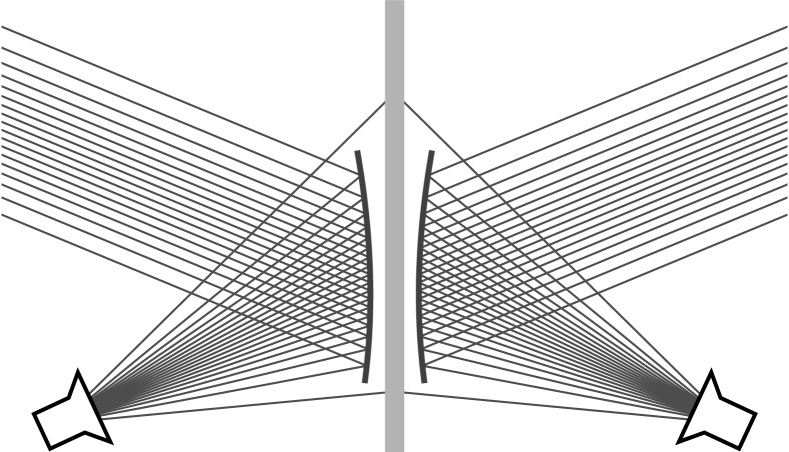
Figure 5: A differential radiometer using back-to-back off-axis paraboloidal dishes. The feeds are designed to mainly illuminate the center of the dishes with minimal spillover past the edges.

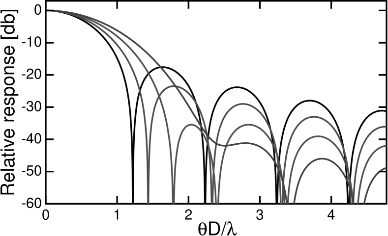
Figure 6: The point spread function of a circular aperture for 4 different values of the edge taper with Gaussian illumination. The four curves are for uniform illumination or 0 db taper, 9, 18 and 27 db taper. The sidelobe level decreases with increasing taper, while the width of the main beam increases slightly.

Experiment to measure smaller angular scales use radio telescopes with dishes to make a beam with a smaller angular spread than a horn. Horns would be used to feed the dishes. A large edge taper should be used to avoid having the beam from the feed spill over the edge of the dish, as seen in Figure 5. Usually there is stuff behind the dish that one would rather not look at, such as the ground or the thermal radiator system in WMAP. Figure 5 illustrates a Gaussian illumination of the primary with the edge of the dish at the 2$\sigma$ point, which corresponds to an edge taper of $e^{-2}$ or about 9 db. Figure 6 shows that sidelobes of a circular aperture with a Gaussian illumination pattern get much smaller for increasing edge taper, and that the angular resolution only declines slightly. WMAP used edge tapers of 13 to 21 db, although the illumination patterns were not symmetric or Gaussian ([Page et al., 2003b]).

The first theoretical predictions of $\Delta T/T=10^{-2}$ ([Sachs and Wolfe, 1967]) and $\Delta T/T=10^{-3.5}$ ([Silk, 1968]) were superseded by predictions based on cold dark matter ([Peebles, 1982], [Bond and Efstathiou, 1987]). These CDM predictions were consistent with the small anisotropy seen by COBE and furthermore predicted a large peak at a particular angular scale due to acoustic oscillations in the baryon/photon fluid prior to recombination. The position of this big peak and other peaks in the angular power spectrum of the CMB anisotropy depends on a combination of the density parameter $\Omega_{m}$ and the vacuum energy density $\Omega_{V}$, so this peak provides a means to determine the density of the Universe ([Jungman et al., 1996]). A tentative detection of the big peak at the position predicted for a flat Universe had been made by 1994 ([Scott et al., 1995]). The peak was localized to $\ell_{pk}=229\pm 8.5$ ([Knox and Page, 2000]) by the beginning of 2000. Later the BOOMERanG group claimed to have made a dramatic improvement in this datum to $\ell_{pk}=197\pm 6$ ([de Bernardis et al., 2000]). This smaller value for $\ell_{pk}$ favored a moderately closed model for the Universe. But improved data on the peak position from WMAP ([Page et al., 2003c]) gives $\ell_{pk}=220.1\pm 0.8$ which is consistent with a flat $\Lambda$CDM model.

Polarization of the CMB was shown to be $<300\;\mu$K ([Lubin and Smoot, 1981]). This observation used a differential polarimeter that was only sensitive to linear polarization. COBE put a limit of $<15\;\mu$K on the polarization anisotropy. The linear polarization of the CMB was first detected by DASIPOL ([Kovac et al., 2002]), and the cross-correlation of the temperature and polarization anisotropies was confirmed by WMAP ([Kogut et al., 2003]).

The detected polarization level is an order of magnitude lower than the anisotropy. The observed polarization is caused by electron scattering during the late stages of recombination on small angular scales and after reionization on large angular scales. The magnitude of the polarization on small angular scales depends on the anisotropy being in place at recombination, as is the case for primordial adiabatic perturbations but not for topological defects; the electron scattering cross-section; and the recombination coefficient of hydrogen. The detection of this polarization is a very strong confirmation of the standard model for CMB anisotropy.

Because polarization is a vector field, two distinct modes or patterns can arise ([Kamionkowski et al., 1997], [Seljak and Zaldarriaga, 1997]): the gradient of a scalar field (the “E” mode) or the curl of a vector field (the “B” mode). Electron scattering only produces the E mode. Electron scattering gives a polarization pattern that is correlated with the temperature anisotropy, so the E modes can be detected by cross-correlating the polarization with the temperature. The B modes cannot be detected this way, and the predicted level of the B modes is at least another order of magnitude below the E modes, or two orders of magnitude below the temperature anisotropy.

2 Observational Techniques

The most important part of any CMB experiment is the modulation scheme that allows one to measure $\mu$K signals in the presence of $\sim 100\;\mbox{K}$ instrumental foregrounds. A good modulation scheme is much more important than high sensitivity, since detector noise can always be beaten down as $1/\sqrt{t}$ by integrating longer, while a systematic error is wrong forever.

Chopping

Figure 7: A total power radiometer with a bolometer [a square-law device indicated by the parabolic curve] feeding a DC amplifier. This design will have too much $1/f$ noise to be useful.

The first step in any modulation scheme is the chopping scheme. The instrument sketched out in Figure 7 will not succeed because the first stage of amplification is at zero frequency (DC), and all electronic circuits suffer from either $1/f$ noise or drifting baselines corresponding to $1/f^{2}$ noise. Figure 7 shows a bolometer detector where the radiation goes directly into a square-law device. In terms of radio engineering, this is similar to the crystal sets that were used in the 1910’s. Modern bolometers running at temperatures below $0.3\;\mbox{K}$ actually have enough sensitivity to make this design superior to radio frequency amplifier designs, but some form of chopping is absolutely required.

Figure 8: A total power radiometer with an AC-biased bolometer feeding an audio amplifier followed by a lockin amplifier. This design is used in BOOMERanG and will be used in the Planck HFI.

The least obtrusive chopping scheme involves biasing the bolometer with alternating current (AC). This is illustrated in Figure 8. The bias supply is connected to an audio frequency (AF) source, shown here as a square wave oscillator, and this causes the responsivity of the bolometer to change sign at an audio frequency rate. The output of the bolometer then goes through an AF amplifier and into a phase sensitive demodulator and low pass filter, or a lockin amplifier. The $1/f$ knee of an AC-biased bolometer can be lower than 0.01 Hz ([Wilbanks et al., 1990]). While AC bias removes the problem of $1/f$ noise due to the amplifier, there can still be $1/f$ or $1/f^{2}$ noise from the atmosphere or drifting temperatures in the instrument. Thus a good scanning strategy is still needed with AC-biased bolometers.

Figure 9: A differential radiometer with an optical chopper so the bolometer looks alternately at two sky different sky positions. The bolometer feeds an audio amplifier followed by a lockin amplifier.

A differential radiometer like the COBE DMR looks alternately at two different sky positions and measures the difference between the brightnesses at these two positions. Figure 9 shows a differential radiometer with a bolometric detector. This system using a chopping secondary is fairly common in infrared astronomy.

Figure 10: A differential radiometer chopping against a load, using an RF amplifier prior to the square-law detector. This kind of instrument is required when measuring the absolute temperature of the CMB, and was used by [Penzias and Wilson, 1965].

Figure 10 shows a radiometer using a radio frequency (RF) amplifier that is chopping against a load. One might think that with the first stage of amplification occuring at a high frequency, chopping would not be necessary, but in practice RF amplifiers have gain fluctuations that contribute multiplicative $1/f$ noise. Chopping against a load is necessary when measuring the absolute temperature of the CMB, $T_{\circ}$.

In terms of antique radio technology, this radiometer with an RF amplifier leading to a square-law device is a tuned RF receiver which was the state-of-the art in 1929. The modern superheterodyne circuit for radio receivers with ampflication and filtering at an intermediate frequency (IF) was used by the COBE DMR, but the primary advantage of a superheterodyne receiver over a tuned RF receiver is its improved selectivity. Since the CMB is a very broad band signal, selectivity beyond that provided by a RF filter is seldom desired.

Figure 11: A dual channel differential radiometer where the chopper acts like a reversing switch. Practical systems with arrays like SCUBA act like this when running with chopper throws smaller than the array.

Finally one can set up a chopping system with two antennae and two amplifier chains, so that the chopper reverses the connections between the horns and the amplifiers. Figure 11 shows such a scheme. In reality this setup would not be very practical, but the same effect is obtained when using an array of detectors like SCUBA behind a chopper with a throw that is less than the size of the array.

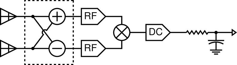
Figure 12: A correlation radiometer where the chopper is replaced by a hybrid circuit. Separate amplifier chains amplify the sum and difference signals which are then multiplied.

A practical microwave radiometer that has the same sensitivity as the system shown in Figure 11 is the correlation radiometer shown in Figure 12. A hybrid circuit at the input forms the sum and difference voltages $(V_{A}+V_{B})/\sqrt{2}$ and $(V_{A}-V_{B})/\sqrt{2}$. These are separately amplified and then multiplied, giving and output proportional to $V_{A}^{2}-V_{B}^{2}$ which is the desired difference in the powers arriving at the two horns.

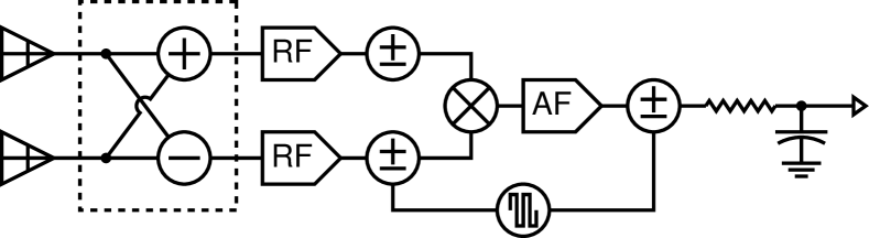
Figure 13: A correlation radiometer with a phase switch inserted in both arms. One of the phase switchs is driven to modulate the output of the multiplier so a lockin amplifier can be used.

There are two practical difficulties with the correlation radiometer. The first is that one will get too much $1/f$ noise from the multiplier and the DC amplifier following it. This can be solved by introducing phase switches into both amplifier chains, and then toggling just one of them. This causes the sign of the output product to toggle, so the output of the multiplier can be amplified at audio frequencies and then fed to a lockin amplifier. This is shown in Figure 13.

The second practical difficulty is the implementation of the multiplier needed for the correlation radiometer. This multiplier has to form a product in a picosecond in order to handle the $94\;\mbox{GHz}$ output of the highest frequency WMAP band. This is handled by using another hybrid followed by square law detectors, which corresponds to using a quarter-square multiplier. The ancient Egyptians used tables of squares to multiply using the formula $A\times B=[(A+B)^{2}-(A-B)^{2}]/4$. Both WMAP and the Planck LFI use this technique, giving what is termed a differential pseudo-correlation radiometer.

These chopping schemes have an effect on the signal-to-noise ratio of the experiment as follows:

• Let the mapping speed of the total power, one-horned system like Figure 8 be 1.00. This is the system planned for the Planck HFI.

• Then the system chopping against a load like Figure 10 spends only 50% of its time looking at the sky, so the sky signal is $\sqrt{2}$ noisier. The noise on the load measurement is also $\sqrt{2}$ noisier because the load is observed only 50% of the time. The difference output is then 2 times noisier, which corresponds to a mapping speed of only 0.25 relative to the total power system.

• The two-horned differential radiometer like Figure 9 is looking at two parts of the sky at once, so it has a mapping speed of 0.5 relative to the total power system.

• The two-horned differential radiometers with two amplifier chains like Figure 11 or Figure 13 achieve a mapping speed equal to the total power system, at the expense of doubling the number of horns and amplifiers. This is the system used by WMAP.

• The Planck LFI is like WMAP but one of the horns is replaced by a load, so its mapping speed is 0.5 relative to the total power system.

Scanning

Any experiment to map $N_{p}$ pixels will need to collect $N_{d}\geq N_{p}$ data points. One would like to see that a typical time history that might be produced by some systematic effect will correspond to an element in the $N_{d}$-dimensional data space that is orthogonal or nearly orthogonal to the $N_{p}$-dimensional subspace that corresponds to the time histories that can be generated by scanning a map. This can be achieved by imposing more than two distinct modulations in the experiment, since the sky is a two dimensional object. For example, the COBE DMR chopped between two beams 100 times per second, spun to interchange those beams every 73 seconds, precessed that spin axis around the circle $94^{\circ}$ away from the Sun every 104 minutes, and then moved that circle around the sky once per year as the Earth went around the Sun. This is a four way modulation. WMAP chops between two beams 2500 times per second, spins to interchange those beams every 132 seconds, precesses its spin axis around a circle $157.5^{\circ}$ from the Sun once per hour, and follows the annual motion of the Sun again giving a four way modulation.

On the other hand ARCHEOPS only scanned around a circle of constant elevation and then let the center of the circle move in right ascension as the Earth turned. This provides only a two way modulation. Since the sky itself is a two dimensional function, just about any time history of drifting baselines is consistent with some pattern on the sky. Thus ARCHEOPS is very vulnerable to striping. This can be seen in the last panel of Figure 2 of astro-ph/0310788 ([Hamilton et al., 2003]) which clearly shows correlated residuals aligned with the scan path. These stripes have a low enough amplitude to not interfere with measurements of the temperature-temperature angular power spectrum $C_{\ell}^{TT}$, but they would ruin a measurement of the polarization power spectrum $C_{\ell}^{EE}$.

Figure 14: The “hourly” scan pattern of COBE, WMAP and Planck from left to right. In each panel the anti-solar direction is in the center, and plus signs denote the North and South ecliptic poles. An equiangular azimuthal projection is used. COBE scanned this area in one orbit of about 103 minutes, WMAP scans its pattern every hour, while Planck spends several hours integrating on one scan circle of radius $70^{\circ}$ radius shown offset from anti-Sun by a $15^{\circ}$ precession angle.

Stripes are caused by small, asymmetric reference sets for pixels in the map. The reference set for the $i^{th}$ pixel consists of the other pixels in the map that are used to establish the baseline for the $i^{th}$ pixel. In a differential experiment like COBE or WMAP the reference set is the circle of radius equal to the chopper throw centered on the $i^{th}$ pixel, or a subset of this circle. This gives a large reference set so differential experiments have nearly uncorrelated noise per pixel and thus no stripes.

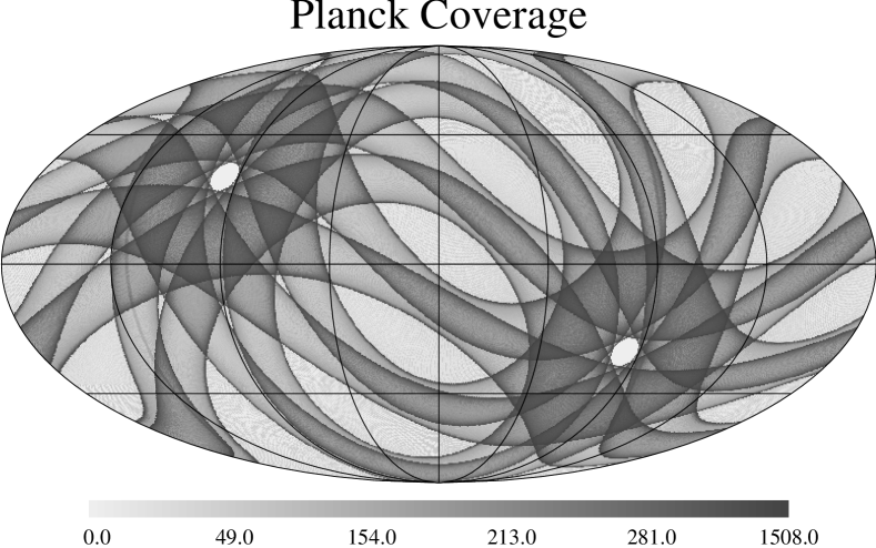
Figure 15: Simulated coverage by the Planck mission assuming a $70^{\circ}$ scan radius and a $15^{\circ}$ precession radius with 10 precession cycles per year. This plot is in galactic coordinates. Note the asymmetry between the coverage patterns in the North and south ecliptic hemispheres.

For a one-horned experiment like ARCHEOPS or Planck the reference set is a line of pixels passing through the $i^{th}$ pixel along the scan direction. The length of the reference set along the scan circle is determined by the $1/f$ knee of the output, and is of order $\pm\omega/f_{knee}$ where $\omega$ is the angular scan rate of the instrument. Observations both before and after the $i^{th}$ pixel can be used to set the baseline so the reference set always has inversion symmetry. A description of the minimum variance method for processing data from one-horned radiometers using a “pre-whitening” filter and time-ordered processing techniques is given by [Wright, 1996]. The width of the pre-whitening filter determines the length of the reference set. When several scan circles pass through the $i^{th}$ pixel in different directions then the reference set becomes larger and more symmetric. If scans pass through the $i^{th}$ pixel in all directions (modulo $180^{\circ}$ because of the inversion symmetry) then the reference set is symmetric and there are no stripes. If $\omega/f_{knee}$ is large and there is a large range of scan angles then the reference set is large and the noise per pixel is nearly uncorrelated.

Figure 16: The path of the Planck scan circle center when the precession angle is $15^{\circ}$ and the precession rate is 10 cycles per year. The difference between the Northern and Southern loops of the cycloid causes the asymmetry in the coverage pattern seen in Figure 15.

Figure 14 shows the amount of sky scanned by COBE, WMAP and Planck in about an hour. These scan patterns move around the sky once per year as the Earth orbits the Sun. The center of the Planck scan circle precesses around the anti-Sun slowly, with perhaps 10 turns per year. The range of scan angles through a pixel is always $180^{\circ}$ for the COBE scan pattern. For the WMAP pattern the region near the ecliptic only sees a range of $45^{\circ}$ in scan angles, while the median range of scan angles is $95^{\circ}$. The median range of scan angles is only $51^{\circ}$ for Planck.

The range of scan angles through a pixel is also crucial in determining the ability of a given experiment to make reliable measurements of polarization. Observing the same pixel with different orientations of the instrumental axes provides the data needed to separate true celestial polarizations from instrumental effects.

The simulated Planck coverage map created while determining the range of scan angles, shown in Figure 15, illustrates an interesting asymmetry that is inherent in this mission’s planned slow precession. If Planck precesses only 10 times per year on a $15^{\circ}$ radius circle, then the scan circle motion due to precession is only 2.5 times higher than the rate due to the annual motion. Thus in one ecliptic hemisphere the net motion is 3.5 times the annual rate while in the opposite hemisphere the net motion is only 1.5 times the annual rate. This results in an asymmetric path for the scan circle center shown in Figure 16. This asymmetry will certainly make testing any North-South asymmetry ([Eriksen et al., 2003]) much more difficult. Planck would have a much better scanning strategy if the precession rate were close to the geometric mean of the spin period and one year. This would be about 10 hours, or several hundred precession periods per year.

Frequency Range

One time history that will always be consistent with a pattern on the sky is obtained by scanning over the Milky Way. The only way to make this nearly orthogonal to a true CMB pattern on the sky is to observe a large range of frequencies. The spectrum of the Milky Way on large angular scales as measured by FIRAS is given in [Wright et al., 1991]. The ratio between the CMB anisotropy signal and this galactic spectrum peaks at $72\;\mbox{GHz}$. For higher frequencies the rising thermal dust emission spectrum starts to dominate over the CMB signal. At frequencies lower than $72\;\mbox{GHz}$ the galactic foreground is dominated by free-free and synchrotron emission. An experiment to measure the primary CMB anisotropy would like to observe a range of frequencies covering $\pm$ a factor of three from $72\;\mbox{GHz}$, or from $24\;\mbox{GHz}$ to $216\;\mbox{GHz}$ But the thermal Sunyaev-Zeldovich effect goes through zero at about $220\;\mbox{GHz}$ so extending the high frequency limit to $400\;\mbox{GHz}$ is clearly a good idea. The WMAP mission only covers the peak and the low frequency side of the peak in the CMB:galaxy ratio, while the Planck mission will extend the high frequency coverage to more than $800\;\mbox{GHz}$.

Sensitivity

Once a good chopping and scanning strategy is planned, a detector system with enough sensitivity to map the CMB anisotropy is needed. The primary anisotropy of the CMB extends up to $\ell\approx 2000$ so there are about 4 million spots on the sky that need to be measured. The anisotropy is about $38\;\mbox{$\mu$K}$ in each spot so the integrated “monopole” sensitivity, $\sigma_{pix}/\sqrt{N_{pix}}$, needs to be about $19\;\mbox{nK}$ in order to reach a signal-to-noise ratio of 1 per spot on the primary anisotropy. A SNR of 1 marks the “point of diminishing returns” when measuring the variance of a Gaussian signal. When the SNR per pixel is $<1$ then the error on $C_{\ell}$ improves like one over the integration time, while when the SNR per pixel is $>1$ then the error on $C_{\ell}$ is limited by cosmic variance and does not improve at all with increased integration time. But to measure E-mode polarization one would like 10 times more sensitivity, and to measure the B-mode polarization one would like at least 100 times more sensitivity.

WMAP will achieve a monopole sensitivity of $23\;\mbox{nK}$ in 4 years which is well into the region of diminishing returns on $C_{\ell}^{TT}$ for the $\ell<900$ range compatible with the WMAP angular resolution. But the WMAP sensitivity is far from the point of diminishing returns for polarization measurements.

How can one reach these sensitivity goals? The goal of a monopole sensitivity of $19\;\mbox{nK}$ can be achieved in one year with a sensitivity of $107\;\mbox{$\mu$K}$ in one second. With a bandwidth of $18\;\mbox{GHz}$ (25% of the $72\;\mbox{GHz}$ optimal frequency) the system temperature requirement is $T_{sys}=14\;\mbox{K}$ for a single radiometer channel, using the Dicke radiometer equation $\Delta T=T_{sys}/\sqrt{Bt}$. The best current performance of High Electron Mobility Transistor (HEMT) amplifiers is about $0.3\;\mbox{K/GHz}$ for cryogenic HEMTs, which is a bit too high. Hence an experiment designed to map the whole sky to the point of diminishing returns for $C_{\ell}^{TT}$ would need to have at least two channels. WMAP has 20 channels with two polarizations on each of the 10 differencing assemblies, but only achieves $1.5\;\mbox{K/GHz}$ with passively cooled HEMTs at running at $\approx 90\;\mbox{K}$. However, the absence of expendable cryogens allows WMAP to operate for several years and easily surpass the sensitivity goal.

The $1/f$ gain fluctuations in HEMTs require a high chopping frequency. Prior to the lockin amplifier, the variance of the output of a HEMT radiometer in a $1\;\mbox{Hz}$ bandwidth ($t_{int}=0.5\;\mbox{sec}$) centered at $f$ is given by

$$\mbox{var}(\Delta T)=\frac{2T_{sys}^{2}}{B}+\left(\frac{\Delta G}{G}(f)\right)^{2}T_{sys}^{2}$$ (1)

The $1/f$ gain fluctuations are given by

$$\left(\frac{\Delta G}{G}(f)\right)^{2}=b^{2}\left(\frac{1\;\mbox{Hz}}{f}\right)^{\alpha}$$ (2)

Typically $\alpha\approx 1$ and $b=10^{-5}/\sqrt{\mbox{Hz}}$ for warm HEMTs and $10^{-4}/\sqrt{\mbox{Hz}}$ for cryogenic HEMTS, and the bandwidth $B$ is 10’s of GHz, so the $1/f$ knee frequency is

$$f_{knee}=(b^{2}B/2)^{1/\alpha}$$ (3)

which ranges from 20 to 1000 Hz for the WMAP radiometers ([Jarosik et al., 2003b]). The chopping frequency $f_{c}$ must be higher than this to avoid excess noise due to gain fluctuations.

The post-lockin noise variance in 1 Hz centered at $f$ is

$$\mbox{var}(\Delta T)=4\,T_{sys}^{2}\left[\frac{2}{B}+\left(\frac{\Delta G}{G}(f_{c})\right)^{2}\right]+T_{off}^{2}\left(\frac{\Delta G}{G}(f)\right)^{2}+\Delta T_{off}(f)^{2}$$ (4)

which still shows $1/f$ noise due to gain fluctuations but they are only driven by the imbalance in the radiometer, $T_{off}$. The factor of “4” in front of $T_{sys}^{2}$ is the increased noise due to chopping. If $T_{off}<<T_{sys}$ then the knee frequency is much lower:

$$f_{knee}^{\prime}=\left(\frac{b^{2}\,B\,T_{off}^{2}}{8\,T_{sys}^{2}\,[1+(f_{knee}/f_{c})^{\alpha}]}\right)^{1/\alpha}.$$ (5)

This is 0.04 Hz for the worst case WMAP radiometer, W4, which has both the highest bandwidth and the highest offset. Ideally the post-lockin $1/f$ knee frequency $f_{knee}^{\prime}$ should be lower than all the scan frequencies but the WMAP spin frequency is only 0.008 Hz so this ideal was not achieved for the W4. $\Delta T_{off}(f)^{2}$ is the power spectrum of the offset drifts which typically show $1/f^{2}$ behavior and dominate the noise at very low frequencies.

Note that the quantum limit on coherent receivers is $0.5h\nu/k$ or $0.024\;\mbox{K/GHz}$ ([Wright, 1999]). This corresponds to 0.5 photons per mode. The $0.3\;\mbox{K/GHz}$ for cryogenic HEMTs is about $7\;\mbox{photons/mode}$. At $72\;\mbox{GHz}$ the CMB has only $\overline{n}=0.4$ photons per mode, where $\overline{n}=(\exp[h\nu/kT]-1)^{-1}$ is the mean number of photons per mode. Thus a background-limited incoherent detector could be much more sensitive than a coherent radiometer using HEMTs.

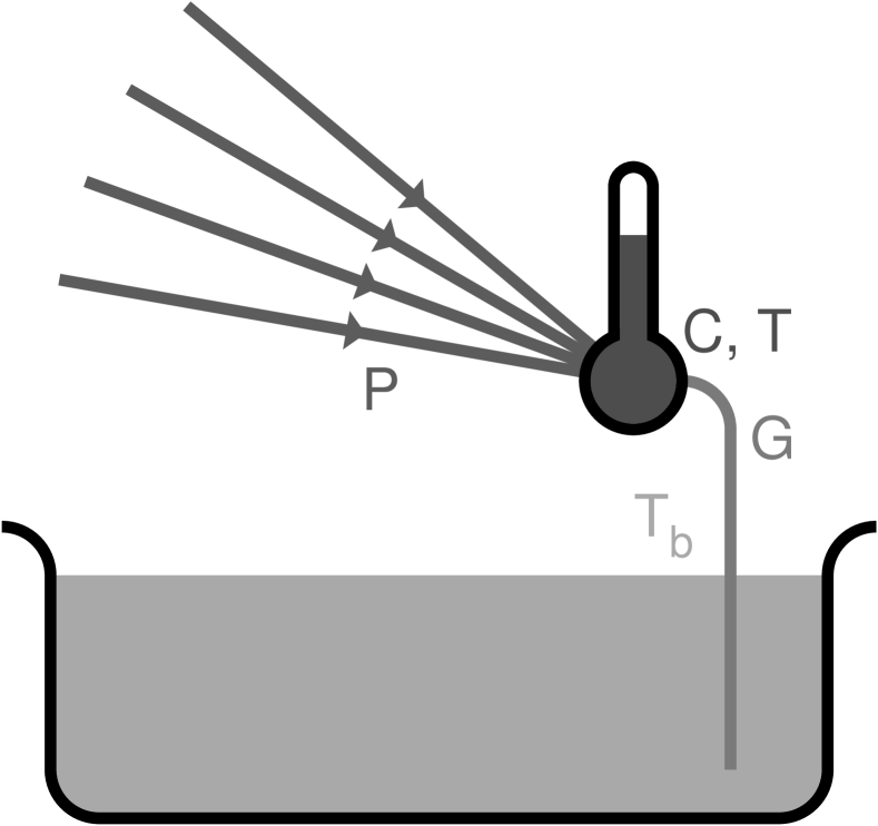
Figure 17: A cartoon representation of a bolometer: a small thermometer at the focus of a beam of radiation, thermally linked to a bath.

Consider a bolometric radiometer with an $18\;\mbox{GHz}$ at $72\;\mbox{GHz}$ with a diffraction-limited throughput, $A\Omega=\lambda^{2}$. A background limited (BLIP) system would have a temperature sensitivity of $19\;\mbox{$\mu$K}$ in 1 second. This is already 6 times better than the $107\;\mbox{$\mu$K}$ in one second needed to reach the point of diminishing returns for $C_{\ell}^{TT}$ with a single channel. However, this bolometer would have to have a noise equivalent power (NEP) less than $7\times 10^{-18}\;\mbox{W/$\sqrt{Hz}$}$, which is still difficult to achieve. The required NEPs are higher and thus easier to achieve at higher frequencies so bolometers are definitely the technology of choice for frequencies higher than $94\;\mbox{GHz}$.

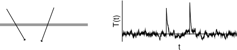
Figure 18: The bolometer shown at left responds to the energy deposited by ionizing particles passing through its absorber, leading the the impulsive signals known as glitches shown at right.

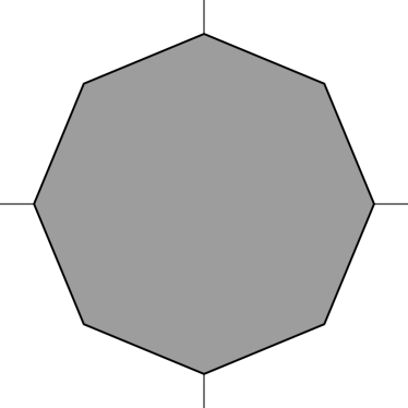
Figure 19: The FIRAS bolometer on the left compared to a spiderweb bolometer on the right.

Bolometers are just thermometers weakly coupled to a thermal bath by a conductance $G$. Radiation is focussed on the bolometer causing its temperature to rise by $\Delta T=P/G$ (see Figure 17). The thermal time constant of a bolometer is given by $\tau=C/G$ where $C=dQ/dT$ is the heat capacity of the bolometer in ergs/K. From the definition of entropy $S=k\ln\Omega$ with $\Omega$ being the state density, and $dS=dQ/T$, we find that

$$\ln\Omega_{bolo}=\ln\Omega_{\circ}+(Q-Q_{\circ})/kT_{b}-0.5(Q-Q_{\circ})^{2}/(kT_{b}^{2}C)+\ldots$$ (6)

where $Q_{\circ}$ is the energy of the bolometer at the bath temperature $T_{b}$, which gives

$$\frac{d\ln\Omega}{dQ}=\frac{1}{kT}=\frac{1}{kT_{b}}\left(1-\frac{Q-Q_{\circ}}{CT_{b}}\right)+\ldots$$ (7)

and thus $T=T_{b}+(Q-Q_{\circ})/C+\ldots$ as required. The thermal bath has a much larger heat capacity so the overal density of states is

$$\Omega_{bolo}\Omega_{bath}\propto\exp[-0.5(Q-Q_{\circ})^{2}/(kT_{b}^{2}C)]$$ (8)

which is a Gaussian with a standard deviation of the energy in the bolometer of $\sigma(Q)=T\sqrt{kC}$. This corresponds to a standard deviation of the power $\sigma(P)=\sigma(Q)/\tau$ and since the noise bandwidth of a simple lowpass filter with time constant $\tau$ is $1/4\tau$, a noise equivalent power of $\mbox{NEP}=T\sqrt{4kC/\tau}$.

Clearly one obtains the best performance for a given time constant with a detector that has the lowest possible heat capacity. The heat capacity of a crystal varies like $C\propto(T/\Theta_{D})^{3}$, where $\Theta_{D}$ is the Debye temperature. Diamond has the highest Debye temperature of any crystal, so FIRAS used an 8 mm diameter, 25 $\mu$m thick disk of diamond as a bolometer ([Mather et al., 1993]). Diamond is transparent, so a very thin layer of gold was applied to give a surface resistance close to the 377 ohms/square impedance of free space. On the back side of the diamond layer an impedance of 267 ohms/square gives a broadband absorbtion. Chromium was alloyed with the gold to stabilize the layer. The temperature of the bolometer was measured with a small silicon resistance thermometer. Running at $T=1.6$ K, the FIRAS bolometers achieved an optical NEP of about $10^{-14}$ W/$\sqrt{Hz}$.

Since $C\propto T^{3}$ and $\mbox{NEP}=T\sqrt{4kC/\tau}$ the NEP scales like $T^{2.5}$. This means that a FIRAS-like bolometer running at 0.1 K could achieve an NEP of $10^{-17}$ W/$\sqrt{Hz}$.

A bolometer is sensitive to any source of heat, not just microwave photons, so charged particles passing through the absorbing layer lead to impulsive signals called glitches as seen in Figure 18. These events occur most frequently at the stratospheric altitudes where balloon-borne experiments operate. An important improvement in bolometer design was the use of mesh absorbers, since there is no need to fill an area $\sim\lambda^{2}$ in order to absorb radiation with wavelength $\lambda$. Figure 19 shows how the area that is sensitive to charged particles can be cut using a spiderweb bolometer ([Bock et al., 1995]). This cuts the mass and hence the heat capacity of the absorber. BOOMERanG used spiderweb bolometers.

Antenna-coupled bolometers ([Schwarz and Ulrich, 1977]) offer another way to achieve a small heat capacity and a small area sensitive to charged particles. Radiation is absorbed by an antenna and then coupled into a transmission line which brings it to a very small absorbing thermometer.

3 Recent Observations

In this paper I will discuss the new observations that have been released in the year prior to this meeting: September 2002 to September 2003. I will discuss these results in time order.

DASIPOL

The Degree Angular Scale Interferometer (DASI) is a very small interferometric array that operates at 26-36 GHz and the South Pole. After measuring the angular power spectrum of the anisotropy ([Halverson et al., 2002]) the instrument was converted into a polarization sensitive interferometer which detected the E mode polarization at 5.5$\sigma$ by looking at a small patch of sky for most of a year of integration time ([Kovac et al., 2002]). The level agreed well with the solid predictions for adiabatic primordial perturbations. Since the measured quantity was the EE autocorrelation, the 5.5$\sigma$ corresponds to a 9% accuracy in the polarization amplitude.

The TE cross-correlation was also seen, but with only 50% accuracy. As expected, the B modes were not seen.

ARCHEOPS

ARCHEOPS is a balloon-borne experiment built to test the detectors and the cryogenic system planned for the ESA Planck Explorer mission High Frequency Instrument. ARCHEOPS has bolometers cooled below 0.1 K, and thus achieves a very high instantaneous sensitivity and was able to map a substantial fraction of the sky with good SNR in only 1 night of observing. This large sky coverage provided a lower level of cosmic or sample variance, so the ARCHEOPS data gave much better results on the low-$\ell$ side of $\ell_{pk}$. This gave a peak location of $\ell_{pk}=220\pm 6$ ([Benoît et al., 2003]).

ACBAR

ACBAR is a bolometric camera array mounted on the VIPER 2 meter diameter telescope at the South Pole. It operates at several frequencies on both sides of the peak of the spectrum of the CMB, and thus can be used to make a sensitive test for the Sunyaev-Zeldovich effect. However, the data released to date are only at one frequency. ACBAR was able to measure the CMB angular power spectrum up to $\ell>2000$ ([Kuo et al., 2002]), but the size of the surveyed regions was so small that ACBAR’s $\ell$ resolution was too limited to provide much information about $\ell_{pk}$. ACBAR was able with its high observing frequency to show that the excess at $\ell>2000$ seen by CBI ([Mason et al., 2003]) is not a primary CMB anisotropy. It could be due to point sources, or it could be due to the S-Z effect, both of which would be much weaker in the ACBAR band than in the CBI 26-36 GHz band.

WMAP

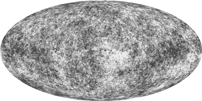
Figure 20: A “no galaxy” map made from an internal linear combination of the 5 WMAP bands, smoothed to $1^{\circ}$ resolution.

Figure 21: Cloud of points from a Monte Carlo Markov chain sampling of the likelihood of models fit to the WMAP plus other CMB datasets. The size of the points indicates how consistent the model is with the HST Key Project on the Distance Scale value for the Hubble constant. The contours show the likelihood computed for 230 Type Ia supernovae ([Tonry et al., 2003]).

The WMAP satellite, launched on 30 June 2001, released it first year results on 11 Feb 2003. Simultaneously the mission was renamed the Wilkinson Microwave Anisotropy Probe to honor the late David T. Wilkinson who was a key member of both the COBE and the WMAP teams until his death in September 2002.

WMAP observed at 5 frequencies: 23, 33, 41, 61 and 94 GHz. From maps in these 5 bands, an internal linear combination map has been constructed that cancels almost all of the Milky Way foreground while preserving the CMB anisotropy. Figure 20 shows this map on a gray scale. All bands were smoothed to $\approx 1^{\circ}$ resolution so the linear combination could be made without worrying about the different beamsizes in the different bands. After this smoothing 53% of the sky was within $\pm 53\;\mu$K of the median of the map, implying an RMS $\Delta T$ of 73 $\mu$K in this smoothing beam. This is considerably higher than the 30 $\mu$K RMS seen by the COBE DMR at a $10^{\circ}$ smoothing because a $1^{\circ}$ beam picks up a large part of the big first acoustic peak.

The WMAP results and their cosmological significance were described in 13 papers and will not be repeated here. [Bennett et al., 2003a] gave a description of the WMAP mission. [Bennett et al., 2003b] summarized the results from first year of WMAP observations. [Bennett et al., 2003c] described the observations of galactic and extragalactic foreground sources. [Hinshaw et al., 2003b] gave the angular power spectrum derived from the the WMAP maps. [Hinshaw et al., 2003a] described the WMAP data processing and systematic error limits. [Page et al., 2003a] discussed the beam sizes and window functions for the WMAP experiment. [Page et al., 2003c] discussed results that can be derived simply from the positions and heights of the peaks and valleys in the angular power spectrum. [Spergel et al., 2003] described the cosmological parameters derived by fitting the WMAP data and other datasets. [Verde et al., 2003] described the fitting methods used. [Peiris et al., 2003] described the consequences of the WMAP results for inflationary models. [Jarosik et al., 2003a] described the on-orbit performance of the WMAP radiometers. [Kogut et al., 2003] described the WMAP observations of polarization in the CMB. [Barnes et al., 2003] described the large angle sidelobes of the WMAP telescopes. [Komatsu et al., 2003] addressed the limits on non-Gaussianity that can be derived from the WMAP data.

Using theWMAP data plus CBI and ACBAR, the position of the big peak in the angular power spectrum was found to be $\ell_{pk}=220.1\pm 0.8$. The position of the big peak defines a track in the $\Omega_{m}$-$\Omega_{V}$ plane shown in Figure 21.

The ratios of the anisotropy powers below the peak at $\ell\approx 50$, at the big peak at $\ell\approx 220$, in the trough at $\ell\approx 412$, and at the second peak at $\ell\approx 546$ were precisely determined using the WMAP data which has a single consistent calibration for all $\ell$’s. Previously, these $\ell$ ranges had been measured by different experiments having different calibrations so the ratios were poorly determined. Knowing these ratios determined the photon:baryon:CDM density ratios, and since the photon density was precisely determined by FIRAS on COBE, accurate values for the baryon density and the dark matter density were obtained. These values are $\Omega_{b}h^{2}=0.0224\pm 4\%$, and $\Omega_{m}h^{2}=0.135\pm 7\%$. The ratio of CDM to baryon densities from the WMAP data is 5.0:1.

Because the matter density $\Omega_{m}h^{2}$ was fairly well constrained by the amplitudes, the positions of a point in Figure 21 served to define a value of the Hubble constant. The size of the points in Figure 21 indicates how well this derived Hubble constant agrees with the $H_{\circ}=72\pm 8$ from the HST Key Project ([Freedman et al., 2001]). Shown as contours are the $\Delta\chi^{2}=1,\;4,\;\&\;9$ contours from my fits to 230 SNe Ia ([Tonry et al., 2003]). Clearly the CMB data, the HST data, and the SNe data are all consistent at a three-way crossing that is very close to the flat Universe line. Assuming the Universe actually is flat, the age of the Universe is very well determined: $13.7\pm 0.2\;\mbox{Gyr}$.

WMAP also found a TE (temperature-polarization) cross-correlation. At small angles the TE amplitude was perfectly consistent with the standard picture of the recombination era. But there was also a large angle TE signal that gave an estimate for the electron scattering optical depth since reionization: $\tau=0.17\pm 0.04$. Based on this the epoch of reionization was 200 million years after the Big Bang.

4 Summary

Measurements of the CMB anisotropy made in the last 5 years have moved cosmology into a new era of precise parameter determination and the ability to probe the conditions during the inflationary epoch. These results depend on the study of perturbations that are still in the linear, small amplitude regime, and thus are not confounded by non-linearities and the difficulties associated with hydrodynamics.