Comparing AMR and SPH Cosmological Simulations: I. Dark Matter & Adiabatic Simulations

Abstract

We compare two cosmological hydrodynamic simulation codes in the context of hierarchical galaxy formation: the Lagrangian smoothed particle hydrodynamics (SPH) code ‘GADGET’, and the Eulerian adaptive mesh refinement (AMR) code ‘Enzo’. Both codes represent dark matter with the N-body method but use different gravity solvers and fundamentally different approaches for baryonic hydrodynamics. The SPH method in GADGET uses a recently developed ‘entropy conserving’ formulation of SPH, while for the mesh-based Enzo two different formulations of Eulerian hydrodynamics are employed: the piecewise parabolic method (PPM) extended with a dual energy formulation for cosmology, and the artificial viscosity-based scheme used in the magnetohydrodynamics code ZEUS. In this paper we focus on a comparison of cosmological simulations that follow either only dark matter, or also a non-radiative (‘adiabatic’) hydrodynamic gaseous component. We perform multiple simulations using both codes with varying spatial and mass resolution with identical initial conditions.

The dark matter-only runs agree generally quite well provided Enzo is run with a comparatively fine root grid and a low overdensity threshold for mesh refinement, otherwise the abundance of low-mass halos is suppressed. This can be readily understood as a consequence of the hierarchical particle-mesh algorithm used by Enzo to compute gravitational forces, which tends to deliver lower force resolution than the tree-algorithm of GADGET at early times before any adaptive mesh refinement takes place. At comparable force resolution we find that the latter offers substantially better performance and lower memory consumption than the present gravity solver in Enzo.

In simulations that include adiabatic gas dynamics we find general agreement in the distribution functions of temperature, entropy, and density for gas of moderate to high overdensity, as found inside dark matter halos. However, there are also some significant differences in the same quantities for gas of lower overdensity. For example, at $z=3$ the fraction of cosmic gas that has temperature $\log T>0.5$ is $\sim 80\%$ for both Enzo/ZEUS and GADGET, while it is $40-60\%$ for Enzo/PPM. We argue that these discrepancies are due to differences in the shock-capturing abilities of the different methods. In particular, we find that the ZEUS implementation of artificial viscosity in Enzo leads to some unphysical heating at early times in preshock regions. While this is apparently a significantly weaker effect in GADGET, its use of an artificial viscosity technique may also make it prone to some excess generation of entropy which should be absent in ENZO/PPM. Overall, the hydrodynamical results for GADGET are bracketed by those for Enzo/ZEUS and Enzo/PPM, but are closer to Enzo/ZEUS.

1 Introduction

Within the currently leading theoretical model for structure formation small fluctuations that were imprinted in the primordial density field are amplified by gravity, eventually leading to non-linear collapse and the formation of dark matter (DM) halos. Gas then falls into the potential wells provided by the DM halos where it is shock-heated and then cooled radiatively, allowing a fraction of the gas to collapse to such high densities that star formation can ensue. The formation of galaxies hence involves dissipative gas dynamics coupled to the nonlinear regime of gravitational growth of structure. The substantial difficulty of this problem is exacerbated by the inherent three-dimensional character of structure formation in a $\Lambda$CDM universe, where due to the shape of the primordial power spectrum a large range of wave modes becomes nonlinear in a very short time, resulting in the rapid formation of objects with a wide range of masses which merge in geometrically complex ways into ever more massive systems. Therefore, direct numerical simulations of structure formation which include hydrodynamics arguably provide the only method for studying this problem in its full generality.

Hydrodynamic methods used in cosmological simulations of galaxy formation can be broken down into two primary classes: techniques using an Eulerian grid, including ‘Adaptive Mesh Refinement’ (AMR) techniques, and those which follow the fluid elements in a Lagrangian manner using gas particles, such as ‘Smoothed Particle Hydrodynamics’ (SPH). Although significant amounts of work have been done on structure/galaxy formation using both types of simulations, very few detailed comparisons between the two simulation methods have been carried out (e.g. Kang et al., 1994; Frenk et al., 1999), despite the existence of widespread prejudices in the field with respect to alleged weaknesses and strengths of the different methods.

Perhaps the most extensive code comparison performed to date was the Santa Barbara cluster comparison project (Frenk et al., 1999), in which several different groups ran a simulation of the formation of one galaxy cluster, starting from identical initial conditions. They compared a few key quantities of the formed cluster, such as radially-averaged profiles of baryon and dark matter density, gas temperature and X-ray luminosity. Both Eulerian (fixed grid and AMR) and SPH methods were used in this study. Although most of the measured properties of the simulated cluster agreed reasonably well between different types of simulations (typically within $\sim 20\%$), there were also some noticeable differences which largely remained unexplained, for example in the central entropy profile, or in the baryon fraction within the virial radius. Later simulations by Ascasibar et al. (2003) compare results from the Eulerian AMR code ART (Kravtsov et al., 2002) with the entropy-conserving version of GADGET. They find that the entropy-conserving version of GADGET significantly improves agreement with grid codes when examining the central entropy profile of a galaxy cluster, though the results are not fully converged. The GADGET result using the new hydro formulation now shows an entropy floor – in the Santa Barbara paper the SPH codes typically did not display any trend towards a floor in entropy at the center of the cluster while the grid-based codes generally did. The ART code produces results that agree extremely well with the grid codes used in the comparison. The observed convergence in cluster properties is encouraging, but there is still a need to explore other systematic differences between simulation methods.

The purpose of the present study is to compare two different types of modern cosmological hydrodynamic methods, SPH and AMR, in greater depth, with the goal of obtaining a better understanding of the systematic differences between the different numerical techniques. This will also help to arrive at a more reliable assessment of the systematic uncertainties in present numerical simulations, and provide guidance for future improvements in numerical methods. The codes we use are ‘GADGET’, an SPH code developed by Springel, Yoshida, & White (2001), and ‘Enzo’, an AMR code developed by Bryan & Norman (1997, 1999). In this paper, we focus our attention on the clustering properties of dark matter and on the global distribution of the thermodynamic quantities of cosmic gas, such as temperature, density, and entropy of the gas. Our work is thus complementary to the Santa Barbara cluster comparison project because we examine cosmological volumes that include many halos and a low-density intergalactic medium, rather than focusing on a single particularly well-resolved halo. We also include idealized tests designed to highlight the effects of artificial viscosity and cosmic expansion.

The present study is the first paper in a series that aims at providing a comprehensive comparison of AMR and SPH methods applied to the dissipative galaxy formation problem. In this paper, we describe the general code methodology, and present fundamental comparisons between dark matter-only runs and runs that include ordinary ‘adiabatic’ hydrodynamics. This paper is meant to provide statistical comparisons between simulation codes, and we leave detailed comparisons of baryon properties in individual halos to a later paper. Additionally, we plan to compare simulations using radiative cooling, star formation, and supernova feedback in forthcoming work.

The organization of this paper is as follows. We provide a short overview of the two codes being compared in Section 2, and then describe the details of our simulations in Section 3. Our comparison is then conducted in two steps. We first compare the dark matter-only runs in Section 4 to test the gravity solver of each code. This is followed in Section 5 with a detailed comparison of hydrodynamic results obtained in adiabatic cosmological simulations. We then discuss effects of artificial viscosity in Section 6, and the timing and memory usage of the two codes in Section 7. Finally, we conclude in Section 8 with a discussion of our findings.

2 Code details

2.1 Adaptive mesh refinement code

‘Enzo’ is an adaptive mesh refinement cosmological simulation code developed by Bryan et al. (Bryan & Norman, 1997, 1999; Norman & Bryan, 1999; Bryan et al., 2001). This code couples an N-body particle-mesh (PM) solver (e.g. Efstathiou et al., 1985; Hockney & Eastwood, 1988) used to follow the evolution of collisionless dark matter with an Eulerian AMR method for ideal gas dynamics by Berger & Colella (1989), which allows extremely high dynamic range in gravitational physics and hydrodynamics in an expanding universe.

Unlike moving mesh methods (Pen, 1995; Gnedin, 1995) or methods that subdivide individual cells (Adjerid & Flaherty, 1998), Berger & Collela’s AMR (also referred to as structured AMR) utilizes an adaptive hierarchy of grid patches at varying levels of resolution. Each rectangular grid patch (referred to as a “grid”) covers some region of space in its parent grid which requires higher resolution, and can itself become the parent grid to an even more highly resolved child grid. ENZO’s implementation of structured AMR places no restrictions on the number of grids at a given level of refinement, or on the number of levels of refinement. However, owing to limited computational resources it is practical to institute a maximum level of refinement $\ell_{\rm max}$.

The Enzo implementation of AMR allows arbitrary integer ratios of parent and child grid resolution. However, in this study we choose to have a refinement factor of two, meaning that each child grid has a factor of two higher spatial resolution than its parent grid. The ratio of boxsize to the maximum grid resolution of a given simulation is therefore $L/e=N_{\rm root}\times 2^{\ell_{\rm max}}$, where $N_{\rm root}$ is the number of cells along one edge of the root grid, and $\ell_{\rm max}$ is the maximum level of refinement allowed.

The AMR grid patches are the primary data structure in Enzo. Each patch is treated as an individual object which can contain both field variables and particle data. Individual grids are organized into a dynamic, distributed hierarchy of mesh patches. Every processor keeps a description of the entire grid hierarchy at all times, so that each processor knows where all grids are. However, baryon and particle data for a given grid only exists on a single processor. The code handles load balancing on a level-by-level basis such that the workload on each level is distributed uniformly across all processors. The MPI message passing library is used to transfer data between processors.

Each grid patch in Enzo contains arrays of values for baryon and particle quantities. The baryon quantities are stored in arrays with the dimensionality of the simulation itself, which can be 1, 2 or 3 spatial dimensions. Grids are partitioned into a core of real zones and a surrounding layer of ghost zones. The real zones store field values and ghost zones are used to temporarily store values which have been obtained directly from neighboring grids or interpolated from a parent grid. These zones are necessary to accommodate the computational stencil of the hydrodynamics solvers (Sections 2.1.1 and 2.1.2) and the gravity solver (Section 2.1.3). The hydro solvers require ghost zones which are three cells deep and the gravity solver requires 6 ghost zones on every side of the real zones. This can lead to significant memory and computational overhead, particularly for smaller grid patches at high levels of refinement.

Since the addition of more highly refined grids is adaptive, the conditions for refinement must be specified. The criteria of refinement can be set by the threshold value of the overdensity of baryon gas or dark matter in a cell (which is really a refinement on the mass of gas or DM in a cell), the local Jeans length, the local density gradient, or local pressure and energy gradients. A cell reaching any or all of these criteria will then be flagged for refinement. Once all cells of given level have been flagged, rectangular boundaries are determined which minimally encompass them. A refined grid patch is introduced within each such bounding rectangle. Thus, the cells needing refinement as well as adjacent cells within the patch which do not need refinement are refined. While this approach is not as memory efficient as cell-splitting AMR schemes, it offers more freedom with finite difference stencils. For example, PPM requires a stencil of seven cells per dimension. This cannot easily be accommodated in cell-splitting AMR schemes. In the current study we use baryon and dark matter overdensities as our refinement criteria.

Two different hydrodynamic methods are implemented in Enzo: the piecewise parabolic method (PPM) developed by Woodward & Colella (1984) and extended to cosmology by Bryan et al. (1995), and the hydrodynamic method used in the magnetohydrodynamics (MHD) code ZEUS. Below, we describe both of these methods in turn, noting that PPM is viewed as the preferred choice for cosmological simulations since it is higher-order-accurate and is based on a technique that does not require artificial viscosity to resolve shocks. Additional physical processes (such as radiative cooling and star formation and feedback) are also implemented within Enzo but are outside the scope of the present comparison study and will not be discussed here.

In Enzo, resolution of the equations being solved is adaptive in time as well as in space. The timestep in Enzo is satisfied on a level-by-level basis by finding the largest timestep such that the Courant condition (and an analogous condition for the dark matter particles) is satisfied by every cell on that level. All cells on a given level are advanced using the same timestep. Once a level $L$ has been advanced in time by $\Delta t_{L}$, all grids at level $L+1$ are advanced, using the same criteria for timestep calculation described above, until they reach the same physical time as the grids at level $L$. At this point grids at level $L+1$ exchange flux information with their parents grids, providing a more accurate solution on level L. This step, controlled by the parameter FluxCorrection in Enzo, is extremely important, and can significantly affect simulation results if not used in an AMR calculation. At the end of every timestep on every level each grid updates its ghost zones by exchanging information with its neighboring grid patches (if any exist) and/or by interpolating from a parent grid. In addition, cells are examined to see if they should be refined or de-refined, and the entire grid hierarchy is rebuilt at that level (including all more highly refined levels). The timestepping and hierarchy advancement/rebuilding process described here is repeated recursively on every level to the specified maximum level of refinement in the simulation.

2.1.1 Hydrodynamics with the piecewise parabolic method

The primary hydrodynamic method used in Enzo is based on the piecewise parabolic method (PPM) of Woodward & Colella (1984) which has been significantly modified for the study of cosmological fluid flows. The method is described in Bryan et al. (1995), but we provide a short description here for clarity. PPM is a higher order-accurate version of Godunov’s method for ideal gas dynamics with third order-accurate piecewise parabolic monotonic interpolation and a nonlinear Riemann solver for shock capturing. It does an excellent job of capturing strong shocks in at most two cells. Multidimensional schemes are built up by directional splitting and produce a method that is formally second order-accurate in space and time which explicitly conserves mass, linear momentum, and energy. The conservation laws for fluid mass, momentum and energy density are written in comoving coordinates for a Friedman-Robertson-Walker space-time. Both the conservation laws and the Riemann solver are modified to include gravity, which is solved using the particle-mesh (PM) technique (see Section 2.1.3). Unlike the other hydrodynamic techniques used in this comparison, PPM does not use artificial viscosity. This is an important methodological difference compared with other methods that use artificial viscosity, such as the ZEUS hydrodynamics algorithm and GADGET’s SPH method.

In order to more accurately treat situations involving bulk hypersonic motion, where the kinetic energy of the gas can dominate the internal energy by many orders of magnitude, both the gas internal energy equation and total energy equation are solved everywhere on the grid at all times. This dual energy formulation ensures that the method produces the correct entropy jump at strong shocks and also yields accurate pressures and temperatures in cosmological hypersonic flows.

2.1.2 The ZEUS hydrodynamic algorithm

As a check on PPM, Enzo also includes an implementation of the finite-difference hydrodynamic algorithm employed in the compressible magnetohydrodynamics code ‘ZEUS’ (Stone & Norman, 1992a, b). Fluid transport is solved on a Cartesian grid using the upwind, monotonic advection scheme of van Leer (1977) within a multistep (operator split) solution procedure which is fully explicit in time. This method is formally second order-accurate in space but first order-accurate in time.

Operator split methods break the solution of the hydrodynamic equations into parts, with each part representing a single term in the equations. Each part is evaluated successively using the results preceding it. The individual parts of the solution are grouped into two steps, called the source and transport steps.

The ZEUS method uses a von Neumann-Richtmyer artificial viscosity to smooth shock discontinuities that may appear in fluid flows and can cause a break-down of finite-difference equations. The artificial viscosity term is added in the source terms as

$$\rho\frac{\partial\textbf{v}}{\partial t} = -\nabla p-\rho\nabla\phi-\nabla\cdot\textbf{Q}$$ (1)

$$\frac{\partial e}{\partial t} = -p\nabla\cdot\textbf{v}-\textbf{Q}:\nabla\textbf{v},$$ (2)

where v is the baryon velocity, $\rho$ is the mass density, $p$ is pressure, $e$ is internal energy density of gas and Q is the artificial viscosity stress tensor, such that:

$$Q_{ii}=\left\{\begin{array}[]{ll}Q_{\rm AV}\rho_{b}(a\Delta v_{i}+\dot{a}\Delta x_{i})^{2},&\textrm{for $a\Delta v_{i}+\dot{a}\Delta x_{i}<0$}\\ 0&\textrm{otherwise}\\ \end{array}\right.$$ (5)

and

$$Q_{ij}=0\;\;\;{\rm for}\;\;i\neq j.$$ (6)

$\Delta x_{i}$ and $\Delta v_{i}$ refer to the comoving width of the grid cell along the $i$-th axis and the corresponding difference in gas peculiar velocities across the grid cell, respectively, and $a$ is the cosmological scale factor. $Q_{\rm AV}$ is a constant with a typical value of 2. We refer the interested reader to Anninos & Norman (1994) for more details.

The limitation of a technique that uses an artificial viscosity is that, while the correct Rankine-Hugoniot jump conditions are achieved, shocks are broadened over 6-8 mesh cells and are thus not treated as true discontinuities. This may cause unphysical pre-heating of gas upstream of the shock wave, as discussed in Anninos & Norman (1994).

2.1.3 The Enzo Gravity Solver

There are multiple methods to compute the gravitational potential (which is an elliptic equation in the Newtonian limit) in a structured AMR framework. One way would be to model the dark matter (or other collisionless particle-like objects, such as stars) as a second fluid in addition to the baryonic fluid and solve the collisionless Boltzmann equation, which follows the evolution of the fluid density in six-dimensional phase space. However, this is computationally prohibitive owing to the large dimensionality of the problem, making this approach unappealing for the cosmological AMR code.

Instead, Enzo uses a particle-mesh N-body method to calculate the dynamics of collisionless systems. This method follows trajectories of a representative sample of individual particles and is much more efficient than a direct solution of the Boltzmann equation in most astrophysical situations. The gravitational potential is computed by solving the elliptic Poisson’s equation:

$$\nabla^{2}\phi=4\pi G\rho,$$ (7)

where $\phi$ is the gravitational potential and $\rho$ is the density of both the collisional fluid (baryonic gas) and the collisionless fluid (dark matter particles).

These equations are finite-differenced and for simplicity are solved with the same timestep as the hydrodynamic equations. This universal timestep is taken to be the minimum of the baryon and dark matter timesteps, thus ensuring numerical stability. The dark matter particles are distributed onto the grids using the cloud-in-cell (CIC) interpolation technique to form a spatially discretized density field (analogous to the baryon densities used to calculate the equations of hydrodynamics). After sampling dark matter density onto the grid and adding baryon density if it exists (to get the total matter density in each cell), the gravitational potential is calculated on the periodic root grid using a fast Fourier transform. In order to calculate more accurate potentials on subgrids, Enzo re-samples the dark matter density onto individual subgrids using the same CIC method as on the root grid, but at higher spatial resolution (and again adding baryon densities if applicable). Boundary conditions are then interpolated from the potential values on the parent grid (with adjacent grid patches on a given level communicating to ensure that their boundary values are the same), and then a multigrid relaxation technique is used to calculate the gravitational potential at every point within a subgrid. Forces are computed on the mesh by finite-differencing potential values and are then interpolated to the particle positions, where they are used to update the particle’s position and velocity information. Potentials on child grids are computed recursively and particle positions are updated using the same timestep as in the hydrodynamic equations. Particles are stored in the most highly refined grid patch at the point in space where they exist, and particles which move out of a subgrid patch are sent to the grid patch covering the adjacent volume with the finest spatial resolution, which may be of the same spatial resolution, coarser, or finer than the grid patch that the particles are moved from. This takes place in a communication process at the end of each timestep on a level.

At this point it is useful to emphasize that the effective force resolution of an adaptive particle-mesh calculation is approximately twice as coarse as the grid spacing at a given level of resolution. The potential is solved in each grid cell; however, the quantity of interest, namely the acceleration, is the gradient of the potential, and hence two potential values are required to calculate this. In addition, it should be noted that the adaptive particle-mesh technique described here is very memory intensive: in order to ensure accurate force resolution at grid edges the multigrid relaxation method used in the code requires a layer of ghost zones which is very deep – typically 6 cells in every direction around the edge of a grid patch. This greatly adds to the memory requirements of the simulation, particularly because subgrids are typically small (on the order of $12^{3}-16^{3}$ real cells for a standard cosmological calculation) and ghost zones can dominate the memory and computational requirements of the code.

2.2 Smoothed particle hydrodynamics code

In this study, we compare Enzo with a new version of the parallel TreeSPH code GADGET (Springel 2005, in preparation), which combines smoothed particle hydrodynamics with a hierarchical tree algorithm for gravitational forces. Codes with a similar principal design (e.g. Hernquist & Katz, 1989; Navarro & White, 1993; Katz et al., 1996; Davé et al., 1997) have been employed in cosmology for a number of years. Compared with previous SPH implementations, the new version GADGET-2 used here differs significantly in its formulation of SPH (as discussed below), in its timestepping algorithm, and in its parallelization strategy. In addition, the new code optionally allows the computation of long-range forces with a particle-mesh (PM) algorithm, with the tree algorithm supplying short-range gravitational interactions only. This ‘TreePM’ method can substantially speed up the computation while maintaining the large dynamic range and flexibility of the tree algorithm.

2.2.1 Hydrodynamical method

SPH uses a set of discrete tracer particles to describe the state of a fluid, with continuous fluid quantities being defined by a kernel interpolation technique if needed (Lucy, 1977; Gingold & Monaghan, 1977; Monaghan, 1992). The particles with coordinates ${\bf r}_{i}$, velocities ${\bf v}_{i}$, and masses $m_{i}$ are best thought of as fluid elements that sample the gas in a Lagrangian sense. The thermodynamic state of each fluid element may either be defined in terms of its thermal energy per unit mass, $u_{i}$, or in terms of the entropy per unit mass, $s_{i}$. We in general prefer to use the latter as the independent thermodynamic variable evolved in SPH, for reasons discussed in full detail by Springel & Hernquist (2002). In essence, use of the entropy allows SPH to be formulated so that both energy and entropy are manifestly conserved, even when adaptive smoothing lengths are used (see also Hernquist, 1993). In the following we summarize the “entropy formulation” of SPH, which is implemented in GADGET-2 as suggested by Springel & Hernquist (2002).

We begin by noting that it is more convenient to work with an entropic function defined by $A\equiv P/\rho^{\gamma}$, instead of directly using the thermodynamic entropy $s$ per unit mass. Because $A=A(s)$ is only a function of $s$ for an ideal gas, we will simply call $A$ the ‘entropy’ in what follows. Of fundamental importance for any SPH formulation is the density estimate, which GADGET calculates in the form

$$\rho_{i}=\sum_{j=1}^{N}m_{j}W(|{\bf r}_{ij}|,h_{i}),$$ (8)

where ${\bf r}_{ij}\equiv{\bf r}_{i}-{\bf r}_{j}$, and $W(r,h)$ is the SPH smoothing kernel. In the entropy formulation of the code, the adaptive smoothing lengths $h_{i}$ of each particle are defined such that their kernel volumes contain a constant mass for the estimated density; i.e. the smoothing lengths and the estimated densities obey the (implicit) equations

$$\frac{4\pi}{3}h_{i}^{3}\rho_{i}=N_{\rm sph}\overline{m},$$ (9)

where $N_{\rm sph}$ is the typical number of smoothing neighbors, and $\overline{m}$ is the average particle mass. Note that in traditional formulations of SPH, smoothing lengths are typically chosen such that the number of particles inside the smoothing radius $h_{i}$ is equal to a constant value $N_{\rm sph}$.

Starting from a discretized version of the fluid Lagrangian, one can show (Springel & Hernquist, 2002) that the equations of motion for the SPH particles are given by

$$\frac{{\rm d}{\bf v}_{i}}{{\rm d}t}=-\sum_{j=1}^{N}m_{j}\left[f_{i}\frac{P_{i}}{\rho_{i}^{2}}\nabla_{i}W_{ij}(h_{i})+f_{j}\frac{P_{j}}{\rho_{j}^{2}}\nabla_{i}W_{ij}(h_{j})\right],$$ (10)

where the coefficients $f_{i}$ are defined by

$$f_{i}=\left[1+\frac{h_{i}}{3\rho_{i}}\frac{\partial\rho_{i}}{\partial h_{i}}\right]^{-1}\,,$$ (11)

and the abbreviation $W_{ij}(h)=W(|{\bf r}_{i}-{\bf r}_{j}|,h)$ has been used. The particle pressures are given by $P_{i}=A_{i}\rho_{i}^{\gamma}$. Provided there are no shocks and no external sources of heat, the equations above already fully define reversible fluid dynamics in SPH. The entropy $A_{i}$ of each particle simply remains constant in such a flow.

However, flows of ideal gases can easily develop discontinuities where entropy must be generated by microphysics. Such shocks need to be captured by an artificial viscosity technique in SPH. To this end GADGET uses a viscous force

$$\left.\frac{{\rm d}{\bf v}_{i}}{{\rm d}t}\right|_{\rm visc.}=-\sum_{j=1}^{N}m_{j}\Pi_{ij}\nabla_{i}\overline{W}_{ij}\,.$$ (12)

For the simulations of this paper, we use a standard Monaghan-Balsara artificial viscosity $\Pi_{ij}$ (Monaghan & Gingold, 1983; Balsara, 1995), parameterized in the following form:

$$\Pi_{ij}=\left\{\begin{tabular}[]{cl}${\left[-\alpha c_{ij}\mu_{ij}+2\alpha\mu_{ij}^{2}\right]}/{\rho_{ij}}$&\mbox{if ${\bf v}_{ij}\cdot{\bf r}_{ij}<0$}\\ 0&\mbox{otherwise},\\ \end{tabular}\right.$$ (13)

with

$$\mu_{ij}=\frac{h_{ij}\,{\bf v}_{ij}\cdot{\bf r}_{ij}}{\left|{\bf r}_{ij}\right|^{2}}.$$ (14)

Here $h_{ij}$ and $\rho_{ij}$ denote arithmetic means of the corresponding quantities for the two particles $i$ and $j$, with $c_{ij}$ giving the mean sound speed. The symbol $\overline{W}_{ij}$ in the viscous force is the arithmetic average of the two kernels $W_{ij}(h_{i})$ and $W_{ij}(h_{j})$. The strength of the viscosity is regulated by the parameter $\alpha$, with typical values in the range $0.75-1.0$. Following Steinmetz (1996), GADGET also uses an additional viscosity-limiter in Eqn. (13) in the presence of strong shear flows to alleviate angular momentum transport.

Note that the artificial viscosity is only active when fluid elements approach one another in physical space, to prevent particle interpenetration. In this case, entropy is generated by the viscous force at a rate

$$\frac{{\rm d}A_{i}}{{\rm d}t}=\frac{1}{2}\frac{\gamma-1}{\rho_{i}^{\gamma-1}}\sum_{j=1}^{N}m_{j}\Pi_{ij}{\bf v}_{ij}\cdot\nabla_{i}\overline{W}_{ij}\,,$$ (15)

transforming kinetic energy of gas motion irreversibly into heat.

We have also run a few simulations with a ‘conventional formulation’ of SPH in order to compare its results with the ‘entropy formulation’. This conventional formulation is characterized by the following differences. Equation (9) is replaced by a choice of smoothing length that keeps the number of neighbors constant. In the equation of motion, the coefficients $f_{i}$ and $f_{j}$ are always equal to unity, and finally, the entropy is replaced by the thermal energy per unit mass as an independent thermodynamic variable. The thermal energy is then evolved as

$$\frac{{\rm d}u_{i}}{{\rm d}t}=\sum_{j=1}^{N}m_{j}\left(\frac{P_{i}}{\rho_{i}^{2}}+\frac{1}{2}\Pi_{ij}\right){\bf v}_{ij}\cdot\nabla_{i}\overline{W}_{ij},$$ (16)

with the particle pressures being defined as $P_{i}=(\gamma-1)\rho_{i}u_{i}$.

2.2.2 Gravitational method

In the GADGET code, both the collisionless dark matter and the gaseous fluid are represented by particles, allowing the self-gravity of both components to be computed with gravitational N-body methods. Assuming a periodic box of size $L$, the forces can be formally computed as the gradient of the periodic peculiar potential $\phi$, which is the solution of

$$\nabla^{2}\phi({\bf x})=4\pi G\sum_{i}m_{i}\left[-\frac{1}{L^{3}}+\sum_{{\bf n}}\tilde{\delta}({\bf x}-{\bf x}_{i}-{\bf n}L)\right],$$ (17)

where the sum over ${\bf n}=(n_{1},n_{2},n_{3})$ extends over all integer triples. The function $\tilde{\delta}({\bf x})$ is a normalized softening kernel, which distributes the mass of a point-mass over a scale corresponding to the gravitational softening length $\epsilon$. The GADGET code adopts the spline kernel used in SPH for $\tilde{\delta}({\bf x})$, with a scale length chosen such that the force of a point mass becomes fully Newtonian at a separation of $2.8\,\epsilon$, with a gravitational potential at zero lag equal to $-Gm/\epsilon$, allowing the interpretation of $\epsilon$ as a Plummer equivalent softening length.

Evaluating the forces by direct summation over all particles becomes rapidly prohibitive for large $N$ owing to the inherent $N^{2}$ scaling of this approach. Tree algorithms such as that used in GADGET overcome this problem by using a hierarchical multipole expansion in which distant particles are grouped into ever larger cells, allowing their gravity to be accounted for by means of a single multipole force. Instead of requiring $N-1$ partial forces per particle, the gravitational force on a single particle can then be computed from just ${\cal O}({\rm log}N)$ interactions.

It should be noted that the final result of the tree algorithm will in general only represent an approximation to the true force described by Eqn. (17). However, the error can be controlled conveniently by adjusting the opening criterion for tree nodes, and, provided sufficient computational resources are invested, the tree force can be made arbitrarily close to the well-specified correct force.

The summation over the infinite grid of particle images required for simulations with periodic boundary conditions can also be treated in the tree algorithm. GADGET uses the technique proposed by Hernquist et al. (1991) for this purpose. Alternatively, the new version GADGET-2used in this study allows the pure tree algorithm to be replaced by a hybrid method consisting of a synthesis of the particle-mesh method and the tree algorithm. GADGET’s mathematical implementation of this so-called TreePM method (Xu, 1995; Bode et al., 2000; Bagla, 2002) is similar to that of Bagla & Ray (2003). The potential of Eqn. (17) is explicitly split in Fourier space into a long-range and a short-range part according to $\phi_{{\bf k}}=\phi^{{\rm long}}_{{\bf k}}+\phi^{{\rm short}}_{{\bf k}}$, where

$$\phi^{{\rm long}}_{{\bf k}}=\phi_{{\bf k}}\exp(-{\bf k}^{2}r_{s}^{2}),$$ (18)

with $r_{s}$ describing the spatial scale of the force-split. This long range potential can be computed very efficiently with mesh-based Fourier methods. Note that if $r_{s}$ is chosen slightly larger than the mesh scale, force anisotropies that exist in plain PM methods can be suppressed to essentially arbitrarily small levels.

The short range part of the potential can be solved in real space by noting that for $r_{s}\ll L$ the short-range part of the potential is given by

$$\phi^{{\rm short}}({\bf x})=-G\sum_{i}\frac{m_{i}}{r_{i}}{\rm erfc}\left(\frac{r_{i}}{2r_{s}}\right).$$ (19)

Here $r_{i}=\min(|{\bf x}-{\bf r}_{i}-{\bf n}L|)$ is defined as the smallest distance of any of the images of particle $i$ to the point ${\bf x}$. The short-range force can still be computed by the tree algorithm, except that the force law is modified according to Eqn. (19). However, the tree only needs to be walked in a small spatial region around each target particle (because the complementary error function rapidly falls for $r>r_{s}$), and no corrections for periodic boundary conditions are required, which together can result in a very substantial performance gain. One typically also gains accuracy in the long range force, which is now basically exact, and not an approximation as in the tree method. In addition, the TreePM approach maintains all of the most important advantages of the tree algorithm, namely its insensitivity to clustering, its essentially unlimited dynamic range, and its precise control about the softening scale of the gravitational force.

3 The simulation set

In all of our simulations, we adopt the standard concordance cold dark matter model of a flat universe with $\Omega_{m}=0.3$, $\Omega_{\Lambda}=0.7$, $\sigma_{8}=0.9$, $n=1$, and $h=0.7$. For simulations including hydrodynamics, we take the baryon mass density to be $\Omega_{b}=0.04$. The simulations are initialized at redshift $z=99$ using the Eisenstein & Hu (1999) transfer function. For the dark matter-only runs, we chose a periodic box of comoving size $12\,{h^{-1}}{\rm\,Mpc}$, while for the adiabatic runs we preferred $3\,{h^{-1}}{\rm\,Mpc}$ to achieve higher mass resolution, although the exact size of the simulation box is of little importance for the present comparison. Note however that this is different in simulations that also include cooling, which imprints additional physical scales. We place the unperturbed dark matter particles at the vertices of a Cartesian grid, with the gas particles offset by half the mean interparticle separation in the GADGET simulations. These particles are then perturbed by the Zel’dovich approximation for the initial conditions. In Enzo, fluid elements are represented by the values at the center of the cells and are also perturbed using the Zel‘dovich approximation.

For both codes, we have run a large number of simulations, varying the resolution, the physics (dark matter only, or dark matter with adiabatic hydrodynamics), and some key numerical parameters. Most of these simulations have been evolved to redshift $z=3$. We give a full list of all simulations we use in this study in Tables 1 and 2 for GADGET and Enzo, respectively; below we give some further explanations for this simulation set.

We performed a suite of dark matter-only simulations in order to compare the gravity solvers in Enzo and GADGET. For GADGET, the spatial resolution is determined by the gravitational softening length $\epsilon$, while for Enzo the equivalent quantity is given by the smallest allowed mesh size $e$ (note that in Enzo the gravitational force resolution is approximately twice as coarse as this: see Section 2.1.3). Together with the boxsize $L_{\rm box}$, we can then define a dynamic range $L_{\rm box}/e$ to characterize a simulation (for simplicity we use $L_{\rm box}/e$ for GADGET as well instead of $L_{\rm box}/\epsilon$). For our basic set of runs with $64^{3}$ dark matter particles we varied $L_{\rm box}/e$ from 256 to 512, 1024, 2048 and 4096 in Enzo. We also computed corresponding GADGET simulations, except for the $L_{\rm box}/e=4096$ case, which presumably would already show sizable two-body scattering effects. Note that it is common practice to run collisionless tree N-body simulations with softenings in the range $1/25-1/30$ of the mean interparticle separation, translating to $L_{\rm box}/e=1600-1920$ for a $64^{3}$ simulation.

Unlike in GADGET, the force accuracy in Enzo at early times also depends on the root grid size. For most of our runs we used a root grid with $64^{3}$ cells, but we also performed Enzo runs with a $128^{3}$ root grid in order to test the effect of the root grid size on the dark matter halo mass function. Both $64^{3}$ and $128^{3}$ particles were used, with the number of particles never exceeding the size of the root grid.

Our main interest in this study lies, however, in our second set of runs, where we additionally follow the hydrodynamics of a baryonic component, modeled here as an ideal, non-radiative gas. As above, we use $64^{3}$ DM particles and $64^{3}$ gas particles (for GADGET), or a $64^{3}$ root grid (for Enzo), in most of our runs, though as before we also perform runs with $128^{3}$ particles and root grids. Again, we vary the dynamic range $L_{\rm box}/e$ from 256 to 4096 in Enzo, and parallel this with corresponding GADGET runs, except for the $L_{\rm box}/e=4096$ case.

An important parameter of the AMR method is the mesh-refinement criterion. Usually, Enzo runs are configured such that grid refinement occurs when the dark matter mass in a cell reaches a factor of 4.0 times the mean dark matter mass expected in a cell at root grid level, or if it has a factor of 8.0 times the mean baryonic mass of a root level cell, but several runs were performed with a threshold density set to 0.5 of the standard values for both dark matter and baryon density. All that the “refinement overdensity” criteria does is set the maximum gas or dark matter mass which may exist in a given cell before that cell must be refined based on a multiple of the mean cell mass on the root grid. For example, a baryon overdensity threshold of 4.0 means that a cell is forced to refine once a cell has accumulated more than 4 times the mean cell mass on the root grid.

When the refinement overdensity is set to the higher value discussed here, the simulation may fail to properly identify small density peaks at early times, so that they are not well resolved by placing refinements on them. As a result, the formation of low-mass DM halos or substructure in larger halos may be suppressed. Note that lowering the refinement threshold results in a significant increase in the number of refined grids, and hence a significant increase in the computational cost of a simulation; i.e., one must tune the refinement criteria to compromise between performance and accuracy.

We also performed simulations with higher mass and spatial resolution, ranging up to $2\times 256^{3}$ particles with GADGET, and $128^{3}$ dark matter particles and a $128^{3}$ root grid with Enzo. For DM-only runs, the gravitational softening lengths in these higher resolution GADGET runs were taken to be $1/30$ of the mean dark matter interparticle separation, giving a dynamic range of $L_{\rm box}/e=3840$ and 7680 for $128^{3}$ and $256^{3}$ particle runs, respectively. For the adiabatic GADGET runs, they were taken to be $1/25$ of the mean interparticle separation, giving $L_{\rm box}/e=3200$ and 6400 for the $128^{3}$ and $256^{3}$ particle runs, respectively. All Enzo runs used a maximum refinement ratio of $L_{\rm box}/e=4096$.

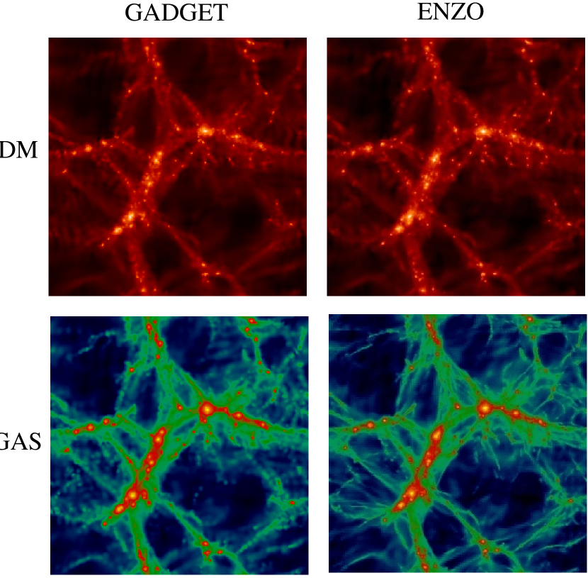
Figure 1: Projected dark matter (top row) and gas mass (bottom row) distribution for GADGET and Enzo in a slab of size $3\times 3\times 0.75\,({h^{-1}}{\rm\,Mpc})^{3}$. For GADGET (left column), we used the run with $2\times 64^{3}$ particles. For Enzo (right column), the run with $64^{3}$ dark matter particles and $128^{3}$ root grid was used.

As an example, we show the spatial distribution of the projected dark matter and gas mass in Figure 1 from one of the representative adiabatic gas runs of GADGET and Enzo. The mass distribution in the two simulations are remarkably similar for both dark matter and gas, except that one can see slightly finer structures in GADGET gas mass distribution compared to that of Enzo. The good visual agreement in the two runs is very encouraging, and we will analyze the two simulations quantitatively in the following sections.

4 Simulations with dark matter only

According to the currently favored theoretical model of the CDM theory, the material content of the universe is dominated by as of yet unidentified elementary particles which interact so weakly that they can be viewed as a fully collisionless component at spatial scales of interest for large-scale structure formation. The mean mass density in this cold dark matter far exceeds that of ordinary baryons, by a factor of $\sim 5-7$ in the currently favored $\Lambda$CDM cosmology. Since structure formation in the Universe is primarily driven by gravity it is of fundamental importance that the dynamics of the dark matter and the self-gravity of the hydrodynamic component are simulated accurately by any cosmological code. In this section we discuss simulations that only follow dark matter in order to compare Enzo and GADGET in this respect.

4.1 Dark matter power spectrum

One of the most fundamental quantities to characterize the clustering of matter is the power spectrum of dark matter density fluctuations. In Figure 2 we compare the power spectra of DM-only runs at redshifts $z=10$ and 3. The short-dashed curve is the linearly evolved power spectrum based on the transfer function of Eisenstein & Hu (1999), while the solid curve gives the expected nonlinear power spectrum calculated with the Peacock & Dodds (1996) scheme. We calculate the dark matter power spectrum in each simulation by creating a uniform grid of dark matter densities. The grid resolution is twice as fine as the mean interparticle spacing of the simulation (i.e. a simulation with $128^{3}$ particles will use a $256^{3}$ grid to calculate the power spectrum) and densities are generated with the triangular-shaped cloud (TSC) method. A fast fourier transform is then performed on the grid of density values and the power spectrum is calculated by averaging the power in logarithmic bins of wavenumber. We do not attempt to correct for shot-noise or the smoothing effects of the TSC kernel.

The results of all GADGET and Enzo runs with $128^{3}$ root grid agree well with each other at both epochs up to the Nyquist wavenumber. However, the Enzo simulations with a $64^{3}$ root grid deviate on small scales from the other results significantly, particularly at $z=10$. This can be understood to be a consequence of the particle-mesh technique adopted as the gravity solver in the AMR code, which induces a softening of the gravitational force on the scale of one mesh cell (this is a property of all PM codes, not just Enzo). To obtain reasonably accurate forces down to the scale of the interparticle spacing, at least two cells per particle spacing are therefore required at the outset of the calculation. In particular, the force accuracy of Enzo is much less accurate at small scales at early times when compared to GADGET because before significant overdensities develop the code does not adaptively refine any regions of space (and therefore increased force resolution to include small-scale force corrections). GADGET is a tree-PM code – at short range, forces on particles are calculated using the tree method, which offers a force accuracy that is essentially independent of the clustering state of the matter down to the adopted gravitational softening length (see Section 2.2.2 for details).

However, as the simulation progresses in time and dark matter begins to cluster into halos, the force calculation by Enzo becomes more accurate as additional levels of grids are adaptively added to the high density regions, reducing the discrepancy seen between Enzo and GADGET at redshift $z=10$ to something much smaller at $z=3$.

4.2 Halo dark matter mass function and halo positions

We have identified dark matter halos in the simulations using a standard friends-of-friends algorithm with a linking length of 0.2 in units of the mean interparticle separation. In this section, we consider only halos with more than 32 particles. We obtained nearly identical results to those described in this section using the HOP halo finder (Eisenstein & Hut, 1998).

In Figure 3, we compare the cumulative DM halo mass function for several simulations with $64^{3}$, $128^{3}$ and $256^{3}$ dark matter particles as a function of $L_{\rm box}/e$ and particle mass. In the bottom panel, we show the residual in logarithmic space with respect to the Sheth-Tormen mass function, i.e., $\log$(N$>$M)$-\log$(S&T). The agreement between Enzo and GADGET simulations at the high-mass end of the mass function is reasonable, but at lower masses there is a systematic difference between the two codes. The Enzo run with $64^{3}$ root grid contains significantly fewer low mass halos compared to the GADGET simulations. Increasing the root grid size to $128^{3}$ brings the low-mass end of the Enzo result closer to that of GADGET.

This highlights the importance of the size of the root grid in the adaptive particle-mesh method based AMR simulations. Eulerian simulations using the particle-mesh technique require a root grid twice as fine as the mean interparticle separation in order to achieve a force resolution at early times comparable to tree methods or so-called P³M methods (Efstathiou et al., 1985), which supplement the softened PM force with a direct particle-particle (PP) summation on the scale of the mesh. Having a conservative refinement criterion together with a coarse root grid in AMR is not sufficient to improve the low mass end of the halo mass function because the lack of force resolution at early times effectively results in a loss of small-scale power, which then prevents many low mass halos from forming.

We have also directly compared the positions of individual dark matter halos identified in a simulation with the same initial conditions, run both with GADGET and Enzo. This run had $64^{3}$ dark matter particles and a $L_{\rm box}=12{h^{-1}}{\rm\,Mpc}$ box size. For GADGET, we used a gravitational softening equivalent to $L_{\rm box}/e=2048$. For Enzo, we used a $128^{3}$ root grid, a low overdensity threshold for the refinement criteria, and we limited refinements to a dynamic range of $L_{\rm box}/e=4096$ (5 total levels of refinement).

In order to match up halos, we apply the following method to identify “pairs” of halos with approximately the same mass and center-of-mass position. First, we sort the halos in order of decreasing mass, and then select a halo from the massive end of one of the two simulations (i.e. the beginning of the list). Starting again from the massive end, we then search the other list of halos for a halo within a distance of $r_{\rm max}=f_{R}\Delta$, where $\Delta$ is the mean interparticle separation ($1/64$ of the boxsize in this case) and $f_{R}$ is a dimensionless number (chosen here to be either 0.5 or 1.0). If the halo masses are also within a fraction $f_{M}$ of one another, then the two halos in question are counted as a ‘matched pair’ and removed from the lists to avoid double-counting. This procedure is continued until there are no more halos left that satisfy these criteria.

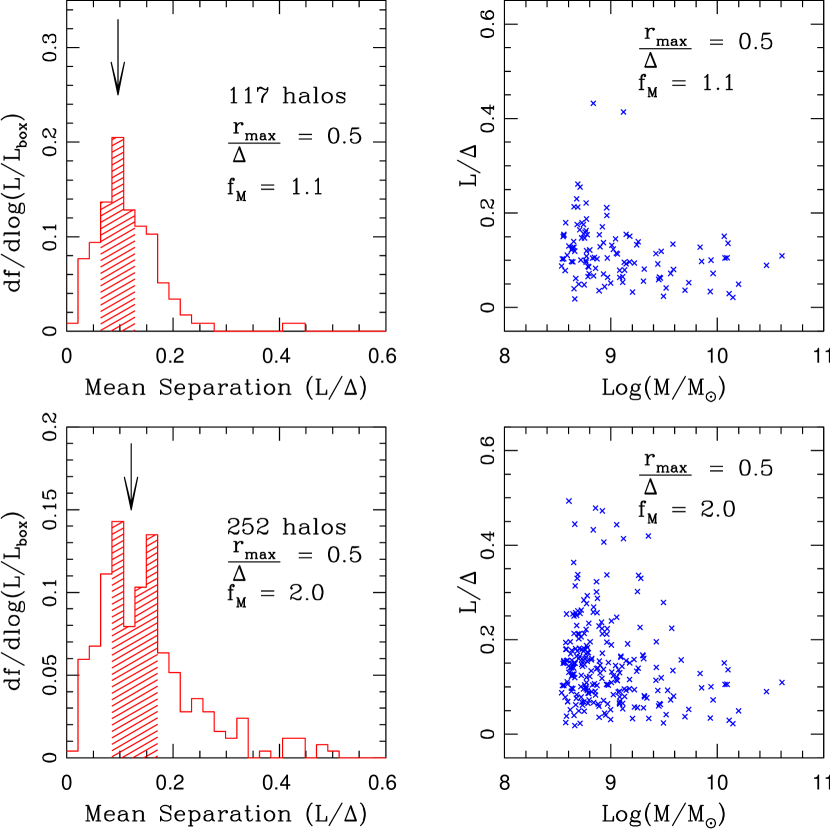
Figure 4: Left column: Probability distribution function of the number of dark matter halos as a function of the separation of the matched halo pair in corresponding Enzo and GADGET simulations (see text for the details of the runs used in this comparison). The separation is in units of the initial mean interparticle separation, $\Delta$ . The shaded region in the distribution function shows the quartiles on both sides of the median value (which is shown by the arrows) of the distribution. Right column: Separation of each pair (in units of $\Delta$) vs. mean halo mass of each pair. The top row is of pairs whose masses agree to within 10% (i.e. $f_{M}=1.1$) and the bottom row is of pairs whose masses agree to within a factor of two (i.e. $f_{M}=2.0$).

In the left column of Figure 4, we show the distribution of pair separations obtained in this way. The arrow indicates the median value of the distribution, and the quartile on each side of the median value is indicated by the shaded region. The values of $r_{\rm max}$ and $f_{M}$ are also shown in each panel. A conservative matching-criterion that allows only a 10% deviation in halo mass and half a cell of variation in the position (i.e. $r_{\rm max}=0.5\Delta$, $f_{M}=1.1$) finds only 117 halo pairs (out of $\sim 292$ halos in each simulation) with a median separation of $0.096\Delta$ between the center-of-mass positions of halos. Increasing $r_{\rm max}$ to $1.0~{}\Delta$ does very little to increase the number of matched halos. Keeping $r_{\rm max}=0.5\Delta$ and increasing $f_{M}$ to 2.0 gives us 252 halo pairs with a median separation of $0.128\Delta$. Increasing $f_{M}$ any further does little to increase the number of matched pairs, and looking further away than $r_{\rm max}=1.0\Delta$ produces spurious results in some cases, particularly for low halo masses.

This result therefore suggests that the halos are typically in almost the same places in both simulations, but that their individual masses show somewhat larger fluctuations. Note however that a large fraction of this scatter simply stems from noise inherent in the group sizes obtained with the halo finding algorithms used. The friends-of-friends algorithm often links (or not yet links) infalling satellites across feeble particle bridges with the halo, so that the numbers of particles linked to a halo can show large variations between simulations even though the halo’s virial mass is nearly identical in the runs. We also tested the group finder HOP (Eisenstein & Hut, 1998), but found that it also shows significant noise in the estimation of halo masses. It may be possible to reduce the latter by experimenting with the adjustable parameters of this group finder (one of which controls the “bridging problem” that the friends-of-friends method is susceptible to), but we have not tried this.

In the right panels of Figure 4, we plot the separation of halo pairs against the average mass of the two halos in question. Clearly, pairs of massive halos tend to have smaller separations than low mass halos. Note that some of the low mass halos with large separation ($L/\Delta>0.4$) could be false identifications. It is very encouraging, however, that the massive halos in the two simulations generally lie within $1/10$ of the initial mean interparticle separation. The slight differences in halo positions may be caused by timing differences between the two simulation codes.

4.3 Halo dark matter substructure

Another way to compare the solution accuracy of the N-body problem in the two codes is to examine the substructure of dark matter halos. The most massive halos in the $128^{3}$ particle dark matter-only simulations discussed in this paper have approximately 11,000 particles, which is enough to marginally resolve substructure. We look for gravitationally-bound substructure using the SUBFIND method described in Springel et al. (2001), which we briefly summarize here for clarity. The process is as follows: a Friends-of-Friends group finder is used (with the standard linking length of 0.2 times the mean interparticle spacing) to find all of the dark matter halos in the simulations. We then select the two most massive halos in the calculation (each of which has at least 11,000 particles in both simulations) and analyze them with the subhalo finding algorithm. This algorithm first computes a local estimate of the density at the positions of all particles in the input group, and then finds locally overdense regions using a topological method. Each of the substructure candidates identified in this way is then subjected to a gravitational unbinding procedure where only particles bound to the substructure are kept. If the remaining self-bound particle group has more than some minimum number of particles it is considered to be a subhalo. We use identical parameters for the Friends-of-Friends and subhalo detection calculations for both the Enzo and GADGET dark matter-only calculations.

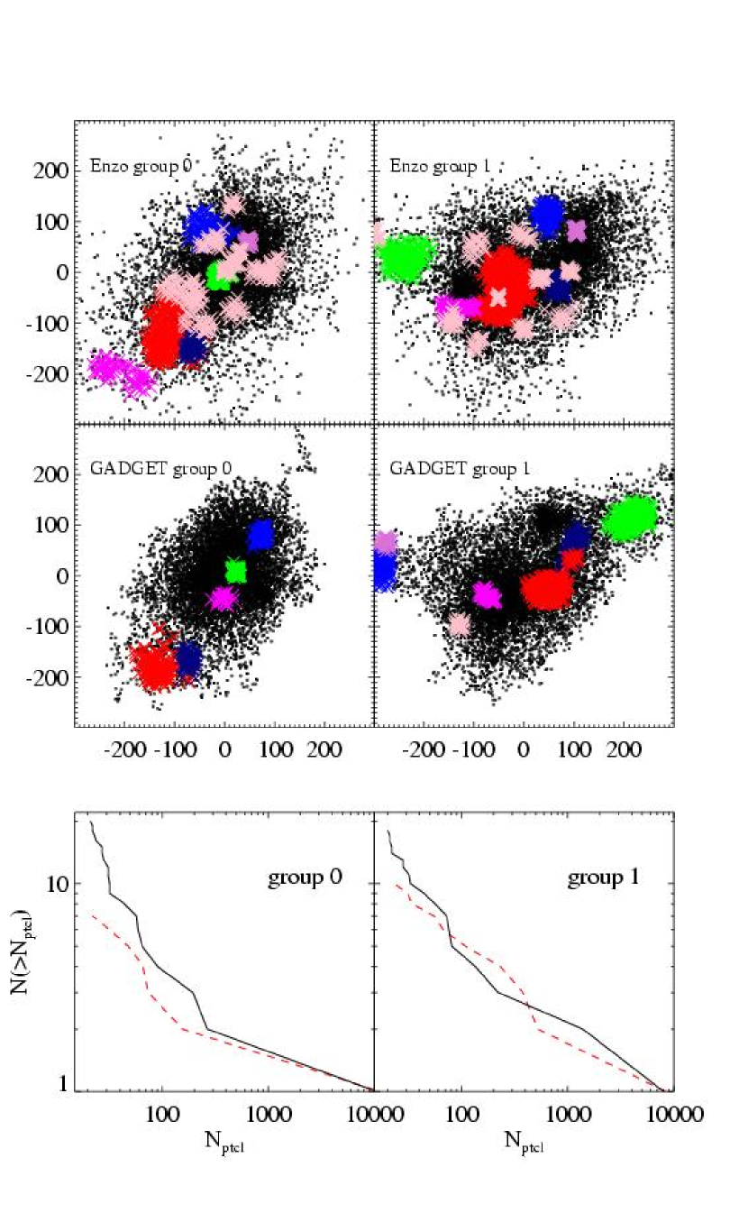
Figure 5: Dark matter substructure in both Enzo and GADGET dark matter-only calculations with $128^{3}$ particles. The Enzo simulations use the “low overdensity” refinement parameters. Left column: data from the most massive halo in the simulation volume. Right column: second most massive halo. Top row: Projected dark matter density for halos in the Enzo simulation with substructure color-coded. Middle row: projected dark matter density for GADGET simulations. Bottom row: Halo substructure mass function for each halo with both Enzo and GADGET results plotted together, with units of number of halos greater than a given mass on the y axis and number of particles on the x axis. In these simulations the dark matter particle mass is $9.82\times 10^{7}~{}M_{\odot}$, resulting in total halo masses of $\sim 10^{12}~{}M_{\odot}$. In the top and middle rows subhalos with the same color correspond to the most massive, second most massive, etc. subhalos. In the Enzo calculation all subhalos beyond the 10th most massive are shown using the same color. Both sets of halos have masses of $\sim 10^{12}~{}M_{\odot}$ The x and y axes in the top two rows are in units of comoving kpc/h. In the bottom row, Enzo results are shown as a black solid line and GADGET results are shown as a red dashed line.

Figure 5 shows the projected dark matter density distribution and substructure mass function for the two most massive halos in the $128^{3}$ particle DM-only calculations for both Enzo and GADGET, which have dark matter masses close to $M_{\rm halo}\sim 10^{12}M_{\odot}$. Bound subhalos are indicated by different colors, with identical colors being used in both simulations to denote the most massive subhalo, second most massive, etc. Qualitatively, the halos have similar overall morphologies in both calculations, though there are some differences in the substructures. The masses of these two parent halos in the Enzo calculation are $8.19\times 10^{11}~{}M_{\odot}$ and $7.14\times 10^{11}~{}M_{\odot}$, and we identify total 20 and 18 subhalos, respectively. The corresponding halos in the GADGET calculation have masses of $8.27\times 10^{11}~{}M_{\odot}$ and $7.29\times 10^{11}~{}M_{\odot}$, and they have 7 and 10 subhalos. Despite the difficulty of Enzo in fully resolving the low-mass end of the halo mass function, the code apparently has no problem in following dark matter substructure within large halos, and hosts larger number of small subhalos than the GADGET calculation. Some corresponding subhalos in the two calculations appear to be slightly off-set. Overall, the agreement of the substructure mass functions for the intermediate mass regime of subhalos is relatively good and within the expected noise.

It is not fully clear what causes the observed differences in halo substructure between the two codes. It may be due to lack of spatial and/or dark matter particle mass resolution in the calculations – typically simulations used for substructure studies have at least an order of magnitude more dark matter particles per halo than we have here. It is also possible that systematics in the grouping algorithm are responsible for some of the differences.

5 Adiabatic simulations

In this section, we start our comparison of the fundamentally different hydrodynamical algorithms of Enzo and GADGET. It is important to keep in mind that a direct comparison between the AMR and SPH methods when applied to cosmic structure formation will always be convolved with a comparison of the gravity solvers of the codes. This is because the process of structure formation is primarily driven by gravity, to the extent that hydrodynamical forces are subdominant in most of the volume of the universe. Differences that originate in the gravitational dynamics will in general induce differences in the hydrodynamical sector as well, and it may not always be straightforward to cleanly separate those from genuine differences between the AMR and SPH methods themselves. Given that the dark matter comparisons indicate that one must be careful to appropriately resolve dark matter forces at early times unless relatively fine root grids are used for Enzo calculations, it is clear that any difference found between the codes needs to be regarded with caution until confirmed with AMR simulations of high gravitational force resolution.

Having made these cautionary remarks, we will begin our comparison with a seemingly trivial test of a freely expanding universe without perturbations, which is useful to check conservation of entropy (for example). After that, we will compare the gas properties found in cosmological simulations of the $\Lambda$CDM model in more detail.

5.1 Unperturbed adiabatic expansion test

Unperturbed ideal gas in an expanding universe should follow Poisson’s law of adiabatic expansion: $T\propto V^{\gamma-1}\propto\rho^{1-\gamma}$. Therefore, if we define entropy as $S\equiv T/\rho^{\gamma-1}$, it should be constant for an adiabatically expanding gas.

This simple relation suggests a straightforward test of how well the hydrodynamic codes described in Section 2 conserve entropy (Hernquist, 1993). To this end, we set up unperturbed simulations for both Enzo and GADGET with $16^{3}$ grid cells or particles, respectively. The runs are initialized at $z=99$ with uniform density and temperature $T=10^{4}\,\rm K$. This initial temperature was deliberately set to a higher value than expected for the real universe in order to avoid hitting the temperature floor set in the codes while following the adiabatic cooling of gas due to the expansion of the universe. The box was then allowed to expand until $z=3$. Enzo runs were performed using both the PPM and ZEUS algorithms and GADGET runs were done with both ‘conventional’ and the ‘entropy conserving’ formulation of SPH.

In Figure 6 we show the fractional deviation from the expected adiabatic relation for density, temperature, and entropy. The GADGET results (left column) show that the ‘entropy conserving’ formulation of SPH preserves the entropy very well, as expected. There is a small net decrease in temperature and density of only $\sim 0.1$%, reflecting the error of SPH in estimating the mean density. In contrast, in the ‘conventional’ SPH formulation the temperature and entropy deviate from the adiabatic relation by 15%, while the comoving density of each gas particle remains constant. This systematic drift is here caused by a small error in estimating the local velocity dispersion owing to the expansion of the universe. In physical coordinates, one expects ${\bf\nabla}\cdot{\bf v}=3H(a)$, but in conventional SPH, the velocity divergence needs to be estimated with a small number of discrete particles, which in general will give a result that slightly deviates from the continuum expectation of $3H(a)$. In our test, this error is the same for all particles, without having a chance to average out for particles with different neighbor configurations, hence resulting in a substantial systematic drift. In the entropy formulation of SPH, this problem is absent by construction.

In the Enzo/PPM run (top right panel), there is a net decrease of only $\sim 0.1$% in temperature and entropy, whereas in Enzo/ZEUS (bottom right panel), the temperature and entropy drop by 12% between $z=99$ and $z=3$. The comoving gas density remains constant in all Enzo runs. In the bottom right panel, the short-long-dashed line shows an Enzo/ZEUS run where we lowered the maximum expansion of the simulation volume during a single timestep (i.e. $\Delta a/a$, where $a$ is the scale factor) by a factor of 10. This results in a factor of $\sim 10$ reduction of the error, such that the fractional deviation from the adiabatic relation is only about 1%. This behavior is to be expected since the ZEUS hydrodynamic algorithm is formally first-order-accurate in time in an expanding universe.

In summary, these results show that both the Enzo/ZEUS hydrodynamic algorithm and the conventional SPH formulation in GADGET have problems in reliably conserving entropy. However, these problems are essentially absent in Enzo/PPM and the new SPH formulation of GADGET.

5.2 Differential distribution functions of gas properties

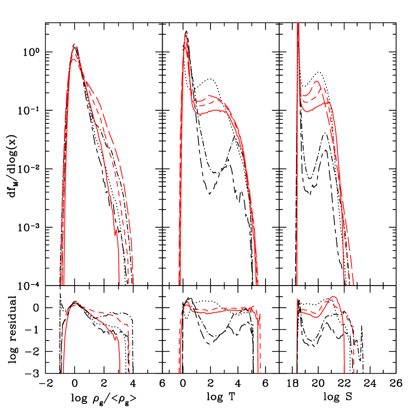
Figure 7: Probability distribution functions of gas mass as functions of gas overdensity (left column), temperature (middle column) and entropy (right column) at $z=10$. For GADGET, runs with $2\times 64^{3}$ (red solid line), $2\times 128^{3}$ (red short-dashed line) and $2\times 256^{3}$ (red long-dashed line) particles are shown. The dynamic range of the Enzo simulations were fixed to $L_{\rm box}/e=4096$, but the particle numbers and the root grid size were varied between $64^{3}$ and $128^{3}$. Both the ZEUS and PPM hydro methods were used in the Enzo calculations. The Enzo line types are: 128g/128dm PPM lowod (black dash-dotted line), 128g/128dm ZEUS (black dotted line), and 64g/64dm PPM lowod (black long dash-short dashed line). In the bottom panels, the residuals in logarithmic scale with respect to the GADGET N256 run are shown.

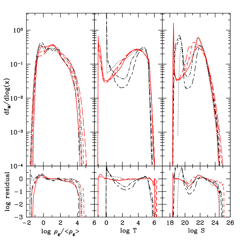
Figure 8: Probability distribution functions of gas mass as functions of gas overdensity (left column), temperature (middle column) and entropy (right column) at $z=3$. For GADGET, runs with $2\times 64^{3}$, $2\times 128^{3}$ and $2\times 256^{3}$ particles were used. The dynamic range of the Enzo simulations were fixed to $L_{\rm box}/e=4096$, but the particle numbers and the root grid size were varied between $64^{3}$ and $128^{3}$ (e.g. 64dm/128grid means $64^{3}$ DM particles and $128^{3}$ root grid). Both the ZEUS and PPM hydro methods were used in the Enzo calculations, as shown in the figure key. Lines are identical to those in Figure 7. In the bottom panels, we show the residuals in logarithmic scale with respect to the GADGET N256 run.

We now begin our analysis of gas properties found in full cosmological simulations of structure formation. In Figures 7 and 8 we show mass-weighted one-dimensional differential probability distribution functions of gas density, temperature and entropy, for redshifts $z=10$ (Figure 7) and $z=3$ (Figure 8). We compare results for GADGET and Enzo simulations at different numerical resolution, and run with both the ZEUS and PPM formulations of Enzo.

At $z=10$, effects owing to an increase of resolution are clearly seen in the distribution of gas overdensity (left column), with runs of higher resolution reaching higher densities earlier than those of lower resolution. However, this discrepancy becomes smaller at $z=3$ because lower resolution runs tend to ‘catch up’ at late times, indicating that then more massive structures, which are also resolved in the lower resolution simulations, become ever more important. One can also see that the density distribution becomes wider at $z=3$ compared to those at $z=10$, reaching to higher gas densities at lower redshift.

At $z=3$, both Enzo and GADGET simulations agree very well at $\log T>3.5$ and $\log S>21.5$, with a characteristic shoulder in the temperature (middle column) and a peak in the entropy (right column) distributions at these values. This can be understood with a simple analytic estimate of gas properties in dark matter halos. We estimate the virial temperature of a dark matter halo with mass $10^{8}\,\rm M_{\odot}$ ($10^{11}\,\rm M_{\odot}$) at $z=3$ to be $\log T=3.7$ ($5.7$). Assuming a gas overdensity of 200, the corresponding entropy is $\log S=21.9$ (23.9). The good agreement in the distribution functions at $\log T>3.5$ and $\log S>21.5$ therefore suggests that the properties of gas inside the dark matter halos agree reasonably well in both simulations. The gas in the upper end of the distribution is in the most massive halos in the simulation, with masses of $\sim 10^{11}\,\rm M_{\odot}$ at $z=3$. Enzo has a built-in temperature floor of $1K$, resulting in an artificial feature in the temperature and entropy profiles at $z=3$. GADGET also has a temperature floor, but it is set to $0.1K$ and is much less noticeable since that temperature is not attained in this simulation. Note that the entropy floor stays at the constant value of $\log S_{\rm init}=18.44$ for all simulations at both redshifts.

However, there are also some interesting differences in the distribution of temperature and entropy between Enzo/PPM and the other methods for gas of low overdensity. Enzo/PPM exhibits a ‘dip’ at intermediate temperature ($\log T\sim 2.0$) and entropy ($\log S\sim 20$), whereas Enzo/ZEUS and GADGET do not show the resulting bimodal character of the distribution. We will revisit this feature when we examine two dimensional phase-space distributions of the gas in Section 5.4, and again in Section 6 when we examine numerical effects due to artificial viscosity. In general, the GADGET results appear to lie in between those obtained with Enzo/ZEUS and Enzo/PPM, and are qualitatively more similar to the Enzo/ZEUS results.

5.3 Cumulative distribution functions of gas properties

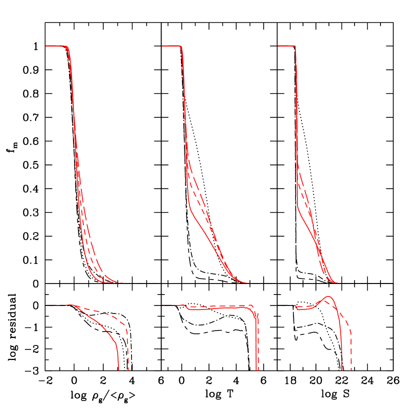
Figure 9: Cumulative distribution functions of gas mass as functions of comoving gas overdensity (left column), temperature (middle column) and entropy (right column) at $z=10$. The simulations and the line types used here are the same as in Figures 7 and 8. In the bottom panels, we show the residuals in logarithmic scale with respect to the GADGET N256 run.

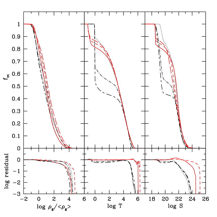
Figure 10: Cumulative distribution functions of gas mass as functions of comoving gas overdensity (left column), temperature (middle column) and entropy (right column) at $z=3$. The simulations and the line types used here are the same as in Figures 7 and 8. In the bottom panels, we show the residuals in logarithmic scale with respect to the GADGET N256 run.

In this section we study cumulative distribution functions of the quantities considered above, highlighting the quantitative differences in the distributions in a more easily accessible way. In Figures 9 and 10 we show the mass-weighted cumulative distribution functions of gas overdensity, temperature and entropy at $z=10$ (Figure 9) and $z=3$ (Figure 10). The measurements parallel those described in Section 5.2, and were done for the same simulations.

We observe similar trends as before. At $z=10$ in the GADGET simulations, 70% of the total gas mass is in regions above the mean density of baryons, but in Enzo, only 50% is in such regions. This mass fraction increases to 80% in GADGET runs, and to 70% in Enzo runs at $z=3$, as more gas falls into the potential wells of dark matter halos.

More distinct differences can be observed in the distribution of temperature and entropy. At $z=10$, only $10-20\%$ of the total gas mass is heated to temperatures above $\log T=0.5$ in Enzo/PPM, whereas this fraction is $70-75\%$ in Enzo/ZEUS, and $35-55\%$ in GADGET. At $z=3$, the mass fraction that has temperature $\log T>0.5$ is $40-60\%$ for Enzo/PPM, and $\sim 80\%$ for both Enzo/ZEUS and GADGET. Similar mass fractions can be observed for gas with entropy $\log S>18.5-19.0$.

In summary, these results show that both GADGET and particularly Enzo/ZEUS tend to heat up a significant amount of gas at earlier times than Enzo/PPM. This may be related to differences in the parameterization of numerical viscosity, a topic that we will discuss in more detail in Section 6.

5.4 Phase diagrams

In Figure 11 we show the redshift evolution of the mass-weighted two-dimensional distribution of entropy vs. gas overdensity for redshifts $z=30$, 10 and 3 (top to bottom rows). Two representative GADGET simulations with $2\times 64^{3}$ and $2\times 256^{3}$ particles are shown in the left two columns. The Enzo simulations shown in the right two columns both have a maximum dynamic range of $L_{\rm box}/e=4096$ and use $128^{3}$ dark matter particles with a $128^{3}$ root grid. They differ in that the simulation in the rightmost column uses the PPM hydrodynamic method, while the other column uses the ZEUS method.

The gas is initialized at $z=99$ at a temperature of $140\,{\rm K}$ and cools as it adiabatically expands. The gas should follow the adiabatic relation until it undergoes shock heating, so one expects that there should be very little entropy production until $z\sim 30$, because the first gravitationally-bound structures are just beginning to form at this epoch. Gas that reaches densities of a few times the cosmic mean is not expected to be significantly shocked; instead, it should increase its temperature only by adiabatic compression. This is true for GADGET and Enzo/PPM, where almost all of the gas maintains its initial entropy, or equivalently, it stays on its initial adiabat. At $z=30$, only a very small amount of high-density gas departs from its initial entropy, indicating that it has undergone some shock heating. However, in the Enzo/ZEUS simulation, a much larger fraction of gas has been heated to higher temperatures. In fact, it looks as if essentially all overdense gas has increased its entropy by a non-negligible amount. We believe this is most likely caused by the artificial viscosity implemented in the ZEUS method, a point we will discuss further in Section 6.

As time progresses, virialized halos and dark matter filaments form, which are surrounded by strong accretion shocks in the gas and are filled with weaker flow shocks (Ryu et al., 2003). The distribution of gas then extends towards much higher entropies and densities. However, there is still a population of unshocked gas, which can be nicely seen as a flat constant entropy floor in all the runs until $z=10$. However, the Enzo/ZEUS simulation largely loses this feature by $z=3$, reflecting its poor ability to conserve entropy in unshocked regions. On the other hand, the GADGET ‘entropy conserving’ SPH-formulation preserves a very well defined entropy floor down to $z=3$. The result of Enzo/PPM lies between that of GADGET and Enzo/ZEUS in this respect. The $1K$ temperature floor in the Enzo code results in an artificial increase in the entropy “floor” in significantly underdense gas at $z=3$.

Perhaps the most significant difference between the simulations lies however in the ‘bimodality’ that Enzo/PPM develops in the density-entropy phase space. This is already seen at redshift $z=10$, but becomes clearer at $z=3$. While Enzo/ZEUS and GADGET show a reservoir of gas around the initial entropy with an extended distribution towards higher density and entropy, Enzo/PPM develops a second peak at higher entropy, i.e. intermediate density and entropy values are comparatively rare. The resulting bimodal character of the distribution is also reflected in a ‘dip’ at $\log T\sim 2.0$ seen in the 1-D differential distribution function in Figures 7 and 8.

We note that the high-resolution GADGET run with $256^{3}$ particles exhibits a broader distribution than the $64^{3}$ run because of its much larger dynamic range and better sampling, but it does not show the bimodality seen in the Enzo/PPM run. We also find that increasing the dynamic range $L_{\rm box}/e$ with a fixed particle number does not change the overall shape of the distributions in a qualitative way, except that the gas extends to a slightly higher overdensity when $L_{\rm box}/e$ is increased.

5.5 Mean gas temperature and entropy

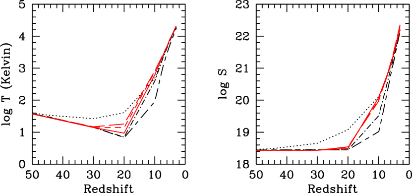
Figure 12: Mass-weighted mean gas temperature and entropy for Enzo and GADGET runs as a function of redshift. The runs used are the same as those shown in Figures 7 and 8.

In Figure 12 we show the mass-weighted mean gas temperature and entropy of the entire simulation box as a function of redshift. We compare results for GADGET simulations with particle numbers of $64^{3}$, $128^{3}$ and $256^{3}$, and Enzo runs with $64^{3}$ or $128^{3}$ particles for different choices of root grid size and hydrodynamic algorithm.

In the temperature evolution shown in the left panel of Figure 12, we see that the temperature drops until $z\sim 20$ owing to adiabatic expansion. This decline in the temperature is noticeably slower in the Enzo/ZEUS runs compared with the other simulations, reflecting the artificial heating seen in Enzo/ZEUS at early times. After $z=20$ structure formation and its associated shock heating overcomes the adiabatic cooling and the mean temperature of the gas begins to rise quickly. While at intermediate redshifts ($z\sim 40-8$) some noticeable differences among the simulations exist, they tend to converge very well to a common mean temperature at late times when structure is well developed. In general, Enzo/PPM tends to have the lowest temperatures, with the GADGET SPH-results lying between those of Enzo/ZEUS and Enzo/PPM.

In the right panel of Figure 12, we show the evolution of the mean mass-weighted entropy, where similar trends as in the mean temperature can be observed. We see that a constant initial entropy ($\log S_{\rm init}=18.44$) is preserved until $z\sim 20$ in Enzo/PPM and GADGET. However, an unphysical early increase in mean entropy is observed in Enzo/ZEUS. The mean entropy quickly rises after $z=20$ owing to entropy generation as a results of shocks occurring during structure formation.

Despite differences in the early evolution of the mean quantities calculated we find it encouraging that the global mean quantities of the simulations agree very well at low redshift, where temperature and entropy converge within a very narrow range. At high redshifts the majority of gas (in terms of total mass) is in regions which are collapsing but still have not been virialized, and are hence unshocked. As we show in Section 6, the formulations of artificial viscosity used in the GADGET code and in the Enzo implementation of the ZEUS hydro algorithm play a significant role in increasing the entropy of unshocked gas which is undergoing compression (though the magnitude of the effect is significantly less in GADGET), which explains why the simulations using these techniques have systematically higher mean temperatures/entropies at early times than those using the PPM technique. At late times these mean values are dominated by gas which has already been virialized in large halos, and the increase in temperature and entropy due to virialization overwhelms heating due to numerical effects. This suggests that most results at low redshift are probably insensitive to the differences seen here during the onset of structure formation at high redshift.

5.6 Evolution of Kinetic Energy

Different numerical codes may have different numerical errors per timestep, which can accumulate over time and results in differences in halo positions and other quantities of interest. It was seen in the Santa Barbara cluster comparison project that each code calculated the time versus redshift evolution in a slightly different way, and overall that resulted in substructures being in different positions because the codes were at different “times”. In our comparison of the halo positions in Section 4.2 we saw something similar – the accumulated error in the simulations results in our halos being in slightly different locations. Since we do not measure the overall integration error in our codes (which is actually quite hard to quantify in an accurate way, considering the complexity of both codes) we argue that the kinetic energy is a reasonable proxy because the kinetic energy is essentially a measure of the growth of structure - as the halos grow and the potential wells deepen the overall kinetic energy increases. If one code has errors that contribute to the timesteps being faster/slower than the other code this shows up as slight differences in the total kinetic energy.

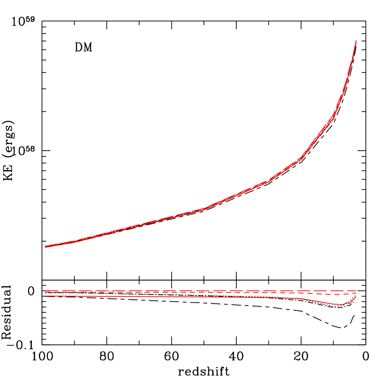
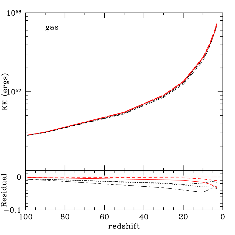
Figure 13: Kinetic energy of dark matter and gas as a function of redshift, and the residuals in logarithmic units with respect to the 256³ particle Gadget run (red long-dashed line) is shown in the bottom panels. Red short-dashed line is for GADGET 128³ particle run, and red solid line is for GADGET 64³ particle run. Black lines are for Enzo runs: 128g128dm PPM, lowod (dot-short dash), 128g128dm Zeus (dotted), 64g64dm PPM, lowod (short dash-long dash).

In Figure 13 we show the kinetic energy (hereafter KE) of dark matter and gas in GADGET and Enzo runs as a function of redshift. As expected, KE increases with decreasing redshift. In the bottom panels, the residuals with respect to the GADGET 256³ particle run is shown in logarithmic units (i.e., $\log$(KE_others) - $\log$(KE₂₅₆) ). Initially at $z=99$, GADGET and Enzo runs agree to within a fraction of a percent within their own runs with different particle numbers. The corresponding GADGET and Enzo runs with the same particle/mesh number agree within a few percent. These differences may have been caused by the numerical errors during the conversion of the initial conditions and the calculation of the KE itself. It is reasonable that the runs with a larger particle number result in a larger KE at both early and late times, because the larger particle number run can sample the power spectrum to a higher wavenumber, therefore having more small-scale power at early times and more small-scale structures at late times. The 64³ runs both agree with each other at $z=99$, and overall have about 1% less kinetic energy than the 256³ run. At the same resolution, Enzo runs show up to a few percent less energy at late times than GADGET runs, but their temporal evolutions track each other closely.

5.7 The gas fraction in halos

The content of gas inside the virial radius of dark matter halos is of fundamental interest for galaxy formation. Given that the Santa Barbara cluster comparison project hinted that there may be a systematic difference between Eulerian codes (including AMR) and SPH codes (Enzo gave slightly higher gas mass fraction compared to SPH runs at the virial radius), we study this property in our set of simulations.

In order to define the gas content of halos in our simulations we first identify dark matter halos using a standard friends-of-friends algorithm. We then determine the halo center to be the center of mass of the dark matter halo and compute the “virial radius” for each halo using Equation (24) of Barkana & Loeb (2000) with the halo mass given by the friends-of-friends algorithm. This definition is independent of the gas distribution, thereby freeing us from ambiguities that are otherwise introduced owing to the different representations of the gas in the different codes on a mesh or with particles. Next, we measure the gas mass within the virial radius of each halo. For GADGET, we can simply count the SPH particles within the radius. In Enzo, we include all cells whose centers are within the virial radius of each halo. Note that small inaccuracies can arise because some cells may only partially overlap with the virial radius. However, in significantly overdense regions the cell sizes are typically much smaller than the virial radius, so this effect should not be significant for large halos.

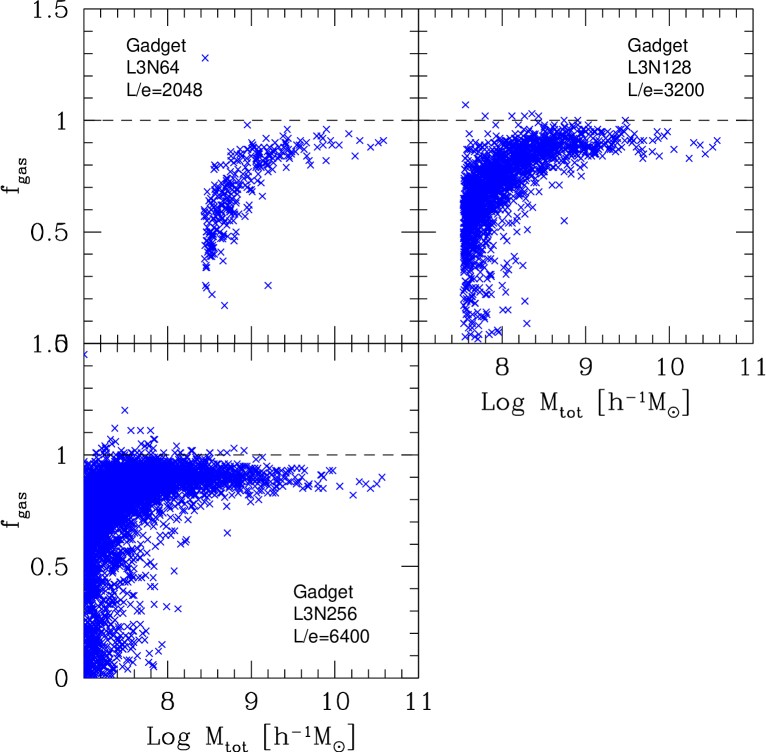
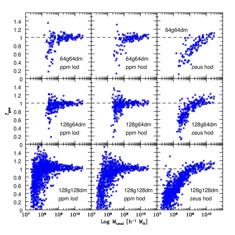
Figure 14: Gas mass fraction normalized by the universal baryon mass fraction $f_{\rm gas}=(M_{\rm gas}/M_{\rm tot})/(\Omega_{b}/\Omega_{m})$ is shown. The top 3 panels are for GADGET runs with $2\times 64^{3}$, ($L_{\rm box}/e=2048$), $2\times 128^{3}$ ($L_{\rm box}/e=3200$), and $2\times 256^{3}$ ($L_{\rm box}/e=6400$) particles. The bottom panels are for the Enzo runs with $64^{3}$ or $128^{3}$ grid, and $64^{3}$ or $128^{3}$ dark matter particles. The ZEUS hydrodynamics method is used for one set of the Enzo simulations (right column) and the PPM method is used for the rest. All Enzo runs have $L_{\rm box}/e=4096$.

In Figure 14 we show the gas mass fractions obtained in this manner as a function of total mass of the halos, with the values normalized by the universal mass fraction $f_{\rm gas}\equiv(M_{\rm gas}/M_{\rm tot})/(\Omega_{b}/\Omega_{m})$. The top three panels show results obtained with GADGET for $2\times 64^{4}$, $2\times 128^{3}$, and $2\times 256^{3}$ particles, respectively. The bottom 9 panels show Enzo results with 64³ and 128³ root grids. Simulations shown in the right column use the ZEUS hydro algorithm and the others use the PPM algorithm. All Enzo runs shown have $64^{3}$ dark matter particles, except for the bottom row which uses $128^{3}$ particles. The Enzo simulations in the top row use a $64^{3}$ root grid and all others use a $128^{3}$ root grid. Grid and particle sizes, overdensity threshold for refinement and hydro method are noted in each panel.

For well-resolved massive halos, the gas mass fraction reaches $\sim 90\%$ of the universal baryon fraction in the GADGET runs, and $\sim 100\%$ in all of the Enzo runs. There is a hint that the Enzo runs seem to give values a bit higher than the universal fraction, particularly for runs using the ZEUS hydro algorithm. This behavior is consistent with the findings of the Santa Barbara comparison project. Given the small size of our sample, it is unclear whether this difference is really significant. However, there is a clear systematic difference in baryon mass fraction between Enzo and GADGET simulations. Examining the mass fraction of simulations to successively larger radii show that the Enzo simulations are consistently close to a baryon mass fraction of unity out to several virial radii, and the gas mass fractions for GADGET runs approaches unity at radii larger than twice the virial radius of a given halo.

The systematic difference between Enzo and GADGET calculations, even for large masses, is also somewhat reflected in the results of Kravtsov et al. (2005). They perform simulations of galaxy clusters done using adiabatic gas and dark matter dynamics with their adaptive mesh code and GADGET. At $z=0$ their results for the baryon fraction of gas within the virial radius converge to within a few percent between the two codes, with the overall gas fraction being slightly less than unity. It is interesting to note that they also observe that the AMR code has a higher overall baryon mass fraction than GADGET, though still slightly less than what we observe with our Enzoresults.

Note that the scatter of the baryon fraction seen for halos at the low mass end is a resolution effect. This can be seen when comparing the three panels with the GADGET results. As the mass resolution is improved, the down-turn in the baryon fraction shifts towards lower mass halos, and the range of halo masses where values near the universal baryon fraction are reached becomes broader. The sharp cutoff in the distribution of the points corresponds to the mass of a halo with 32 DM particles.

It is also interesting to compare the cumulative mass function of gas mass in halos, which we show in Figure 15 for adiabatic runs. This can be viewed as a combination of a measurement of the DM halo mass function and the baryon mass fractions. In the lower panel, the residuals in logarithmic scale are shown for each run with respect to the Sheth & Tormen (1999) mass function (i.e., $\log$(N[$>$M])$-\log$(S&T)).

As with the dark matter halo mass function, the gas mass functions agree well at the high-mass end over more than a decade of mass, but there is a systematic discrepancy between AMR and SPH runs at the low-mass end of the distribution. While the three SPH runs with different gravitational softening agree well with the expectation based on the Sheth & Tormen mass function and an assumed universal baryon fraction at $M_{\rm gas}<10^{8}\,{h^{-1}}\,\rm M_{\odot}$, the Enzo run with $64^{3}$ root grid and $64^{3}$ DM particles has fewer halos. Similarly, the Enzo run with $128^{3}$ grid and $128^{3}$ DM particles has fewer low mass halos at $M_{\rm gas}<10^{7}\,{h^{-1}}\,\rm M_{\odot}$ compared to the GADGET $128^{3}$ DM particle run. Convergence with the SPH results for Enzo requires the use of a root grid with spatial resolution twice that of the initial mean interparticle separation, as well as a low-overdensity refinement criterion. We also see that the PPM method results in a better gas mass function than the ZEUS hydro method at the low-mass end for the same number of particles and root grid size.

6 The role of artificial viscosity

In Section 5.4 we found that slightly overdense gas in Enzo/ZEUS simulations shows an early departure from the adiabatic relation towards higher temperature, suggesting an unphysical entropy injection. In this section we investigate to what extent this effect can be understood as a result of the numerical viscosity built into the ZEUS hydrodynamic algorithm. As the gas in the pre-shocked universe begins to fall into potential wells, this artificial viscosity causes the gas to be heated up in proportion to its compression, potentially causing a significant departure from the adiabat even when the shock has not occurred yet; i.e. when the compression is only adiabatic.

This effect is demonstrated in Figure 16, where we compare two-dimensional entropy–overdensity phase space diagrams for two Enzo/ZEUS where the strength of the artificial viscosity was reduced from its “standard” value of $Q_{\rm AV}=2.0$ to $Q_{\rm AV}=0.5$. These runs used $64^{3}$ dark matter particles and $64^{3}$ root grid, and the $Q_{\rm AV}=2.0$ corresponds to the case shown earlier in Figure 11.

Comparison of the Enzo/ZEUS runs with $Q_{\rm AV}=0.5$ and 2.0 shows that decreasing $Q_{\rm AV}$ results in a systematic decrease of the unphysical gas heating at high redshifts. Also, at $z=4$ the $Q_{\rm AV}=0.5$ result shows a secondary peak at higher density, so that the distribution becomes somewhat more similar to the PPM result. Unfortunately, a strong reduction of the artificial viscosity in the ZEUS algorithm is numerically dangerous because the discontinuities that can appear owing to the finite-difference method are then no longer smoothed sufficiently by the artificial viscosity algorithm, which can produce unstable or incorrect results.

An artificial viscosity is needed to capture shocks when they occur in both the Enzo/ZEUS and GADGET SPH scheme. This in itself is not really problematic, provided the artificial viscosity is very small or equal to zero in regions without shocks. In this respect, GADGET’s artificial viscosity behaves differently from that of Enzo/ZEUS. It takes the form of a pairwise repulsive force that is non-zero only when Lagrangian fluid elements approach each other in physical space. In addition, the strength of the force depends in a non-linear fashion on the rate of compression of the fluid. While even an adiabatic compression produces some small amount of (artificial) entropy, only a compression that proceeds rapidly with respect to the sound-speed, as in a shock, produces entropy in large amounts. This can be seen explicitly when we analyze equations (13) and (15) for the case of a homogeneous gas which is uniformly compressed. For definiteness, let us consider a situation where all separations shrink at a rate $q=\dot{r}_{ij}/r_{ij}<0$, with ${\bf\nabla}\cdot{\bf v}=3\,q$. It is then easy to show that the artificial viscosity in GADGET produces entropy at a rate

$$\frac{{\rm d}\log A_{i}}{{\rm d}\log\rho_{i}}=\frac{\gamma-1}{2}\alpha\left[\frac{-q\,h_{i}}{c_{i}}+2\left(\frac{q\,h_{i}}{c_{i}}\right)^{2}\right].$$ (20)

Note that since we assumed a uniform gas, we here have $h_{i}=h_{ij}$, $c_{i}=c_{ij}$, and $\rho_{i}=\rho_{ij}$. We see that only if the compression is fast compared to the sound-crossing time across the typical spacing of SPH particles, i.e. for $|q|>c_{i}/h_{i}$, a significant amount of entropy is produced, while slow (and hence adiabatic) compressions proceed essentially in an isentropic fashion. On the other hand, the artificial viscosity implemented in Enzo/ZEUS produces entropy irrespective of the sound-speed, depending only on the compression factor of the gas.

We have also investigated the pre-shock entropy generation in Enzo/ZEUS using another simple test, the collapse of a one-dimensional Zel’dovich pancake. The initial conditions of this test are simple and described in full detail in Bryan et al. (1995). A one-dimensional simulation volume is set up in an expanding coordinate system in a flat cosmology with an initially sinusoidal density perturbation with a peak at $x=0.5$ and a corresponding perturbation in the velocity field with nodes at $x=0.0$, 0.5, and 1.0. A temperature perturbation is added such that gas entropy is constant throughout the volume.

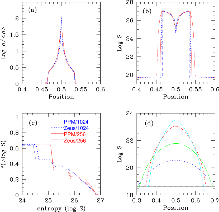
Figure 17: Final results of the Zel’dovich pancake test. Panel (a): Log baryon overdensity vs. position. Panel (b): Log entropy vs. position. Panel (c): Cumulative mass-weighted entropy distribution function. Panel (d): Pre-shock entropy evolution in the 256-cell Zeus run. All Zel’dovich pancake simulations are performed in one dimension using the Enzo code. Panels (a), (b), (c): The line types are for PPM/1024 (short-dashed), PPM/256 (solid), ZEUS/1024 (dotted), and ZEUS/256 (long dashed) where 256 and 1024 are the number of cells used in the calculation. All data is at the end of the run $(z=0)$. Panel (d): Entropy evolution of the 256-cell ZEUS and PPM runs for redshifts $z=20$ (black), 10 (blue dotted), 5 (green long-dashed), 2.5 (red dot-dashed) and 2 (cyan dot-long-dashed). All PPM results overlay the ZEUS initial conditions $(z=20)$. Note that the x-axis range for panel (d) is different from that of panels (a) and (b).

In Figure 17 we show the density and entropy profiles as a function of position, at a time when the non-linear collapse of the pancake is well underway. We also show the pre-shock evolution of the entropy profile for both algorithms. We compare runs using 256 and 1024 grid cells with both the ZEUS and PPM formulations of Enzo.

As the matter falls in onto the density peak at $x=0.5$, accretion shocks on either side form, clearly marked by the jumps in density, entropy, and temperature. Note that the dip in the temperature at $x=0.5$ is physical – the gas sitting there is unshocked and only adiabatically compressed, and therefore has relatively low temperature. Reassuringly, both the ZEUS and PPM hydrodynamical methods reproduce the qualitative behavior of the Zel’dovich pancake quite well, but there are also some systematic differences at a given resolution. This can be seen most clearly in the mass-weighted cumulative entropy distribution in the bottom left panel of Figure 17. We see that the Enzo/ZEUS calculations show a broader distribution than Enzo/PPM for a given spatial resolution. This can be interpreted as another sign of pre-shock entropy generation by the artificial viscosity in ZEUS. In contrast, the Riemann solver used in PPM can capture shocks such that they are resolved as true discontinuities, which avoids this problem.

More concrete evidence of spurious entropy generation in the artificial viscosity-based scheme can be seen by examining the pre-shock evolution of entropy in these simulations (as seen in panel (d) of Figure 17). No entropy should be generated before the twin shocks form to the left and right of $x=0.5$ (as can be seen in panel (b) of the same figure). The simulations using PPM (black solid line in panel d) produce no spurious entropy. The simulations using the ZEUS scheme, however, produce significant amounts of entropy in the infalling (but unshocked) gas. Note that the magnitude of the entropy generation is relatively small compared to the final entropy produced in the shocks (as seen in panel ($b$)), but the values are still significant.

While this test showed only comparatively small differences between the different methods, it is plausible that the effects of pre-shock entropy generation become much more important in three-dimensional cosmological simulations, where galaxies form hierarchically through complicated merger processes that involve extremely complex shock patterns. We thus speculate that this effect may be the key reason for the systematic differences between the Enzo/PPM runs and the ZEUS and GADGET simulations.

7 Timing & memory usage

An important practical consideration when assessing the relative performance of computational methods or simulation codes is the amount of computational resources they require to solve a given problem. Of primary importance are the total amount of memory and the CPU time that is needed. However, it is not always easy to arrive at a meaningful comparison, particularly for very different methods such as AMR and SPH. For example, the variable number of grid cells owing to the adaptive nature of AMR is an important complication, making the number of resolution elements change over time, while the particle number stays constant in the SPH method. An additional layer of complexity is added when considering parallel codes. The parallelization strategies that are used for AMR applications can be significantly different than those used in SPH codes, and the performance of an individual simulation code can heavily depend on the specific computer architecture and implementation of MPI (or other software used for parallelization) chosen. Therefore we caution the readers to take all of the timing information discussed in this section as results for a particular problem setup and machine architecture, and not to extrapolate directly to different types of cosmological simulations (e.g., with cooling and star formation) and machines.

7.1 Initial comparison on a distributed memory machine

When we started this project, we initially performed our comparison runs on the IA-64 Linux cluster Titan at the National Center for Supercomputing Applications (NCSA). It had 134 dual processor nodes with 800 MHz Intel Itanium 1 chips, 2.5 GB memory per node, and Myrinet 2000 network interconnect. Our initial comparison on Titan showed that the GADGET code was faster than Enzo by a factor of 40 (15) for a 64³ (128³) particle DM-only run when Enzo was using a low overdensity criteria for grid refinement. The low overdensity refinement criterion was required for Enzo in order to obtain a DM halo mass function comparable to that of GADGET at low-mass end. GADGET used a factor of 18 (4) less amount of memory than Enzo for a 64³ (128³) particle DM-only run. For the adiabatic runs, GADGET was faster than Enzo by a factor of 2.5 for a $64^{3}$ DM particles and 64³ gas particles (a 64³ root grid for Enzo). A GADGET run with 128³ dark matter and gas particles completed 8 times faster than an Enzo simulation with a 128³ root grid and 64³ DM particles. These performance results were gathered using Linux-based Beowulf-style clusters with relatively slow inter-node communication networks. Since the AMR code performs load balancing by passing grids between processors, it was expected that the performance of Enzo would improve on a large shared-memory machine. The disparity is most significant for DM-only simulations, so improvement of the Enzo N-body solver could significantly increase the performance of the AMR code.

7.2 More recent comparison on a shared memory machine

During the course of this comparison study, both GADGET and Enzo evolved, and the performance of both codes have greatly improved. Therefore, we repeated the performance comparison with our updated codes using the IBM DataStar machine at the San Diego Supercomputing Center. The portion of the machine used for these timing tests is composed of 176 IBM p655 compute nodes, each of which has eight 1.5 GHz IBM Power4 processors. These processors are super-scalar, pipelined 64 bit chips which can execute up to 8 instructions per clock cycle and up to four floating point operations per clock cycle, with a theoretical peak performance of 6.0 GFlop per chip. Processors in a single node share a total of 16 GB of memory. All nodes are connected by an IBM Federation switch, which provides processor-to-processor bandwidth of approximately 1.4 GB/s with 8 microsecond latency when using IBM’s MPI library. Each node is directly connected to a parallel filesystem through a Fibre Channel link.

We first compare the series of dark matter-only runs discussed in Section 4. A GADGET simulation with $64^{3}$ dark matter particles takes total wall-clock time of 225 seconds on 8 cpus (total 1800 seconds CPU time) and requires 270 MB of memory. 24% of the total computational time was spent doing interprocessor message-passing. The corresponding Enzo simulation with $64^{3}$ particles and a $64^{3}$ root grid requires 1053 seconds on 8 cpus (total 8424 seconds CPU time) when refining on a dark matter overdensity of 2.0, and requires 1.21 GB of memory total. 34% of the total computational time was spent in interprocessor communication. This is a factor of 4.7 slower than the corresponding GADGET simulation, and requires roughly 4.5 times more memory. Raising the refinement criteria to a dark matter overdensity of 4.0 (at a cost of losing low-mass DM halos) reduces the wall clock time to 261 seconds on 8 processors (total 2088 seconds CPU time) and decreases the total amount of memory needed to 540 MB, which is comparable to the GADGET simulation. A $128^{3}$ DM particle GADGET adiabatic run takes a total of 2871 seconds to run on 8 cpus (total 22,968 seconds CPU time) and requires 1.73 GB of memory. An Enzo simulation with $128^{3}$ particles and a $128^{3}$ root grid that refines on a dark matter overdensity of 2.0 needs approximately 34,028 seconds on 8 processors (total 272,224 CPU seconds) and 5.6 GB of memory. This is a factor of 12 slower and 3.2 times more memory than the equivalent GADGET run. The same calculation run with refinement overdensities of 4.0 or 8.0 completes in 13,960 and 3839 seconds, respectively, which are factors of 4.9 and 1.3 slower than the equivalent GADGET run. The reason for the huge change in computational speeds is due to the low overdensity threshold used in the first simulation, which results in a huge number of grids to be instantiated and a great deal of time to be spent regridding the simulation. Raising the overdensity criteria suppresses the formation of halos at the low mass end of the mass function, though higher-mass halos are unaffected. This timing comparison suggests that if one is interested in simulating the full spectrum of dark matter halos at a reasonable computational cost, GADGET would be a wiser choice than Enzo for this application. If one was interested in only the high-mass end of the mass function, the codes have comparable performance.

Comparison of the adiabatic gas + N-body cosmological simulations in Section 5 is also quite informative. The $64^{3}$ dark matter particle/$64^{3}$ gas particle GADGET calculation takes 1839 seconds to run on 8 processors (total 14,712 seconds CPU time) and requires 511 MB of memory. The equivalent Enzo simulation with $64^{3}$ particles and a $64^{3}$ root grid using the low overdensity refinement criteria (refining on a baryon overdensity of 4.0 and a dark matter overdensity of 2.0) requires 6895 seconds on 8 processors (55,160 seconds total) and 2.5 GB of memory. This is 3.7 times slower and 4.9 times more memory than the corresponding GADGET run. Raising the overdensity thresholds by a factor of two decreases the computational time to 2168 seconds on 8 processors and the memory required to 1.28 GB. The GADGET calculation with $128^{3}$ dark matter and baryon particles requires 35,879 seconds on 8 cpus (287032 seconds total CPU time) and 5.4 GB of memory, and an Enzo calculation with $128^{3}$ particles on a $128^{3}$ root grid which refines on a baryon overdensity of 8.0 and a dark matter overdensity of 4.0 requires 64,812 seconds and 8 GB of memory. Enzo simulations using the PPM and Zeus hydro methods require comparable amounts of simulation time.

8 Conclusions

This paper presents initial results of a comparison of two state-of-the-art cosmological hydrodynamic codes: Enzo, an Eulerian adaptive mesh refinement code, and GADGET, a Lagrangian smoothed particle hydrodynamics code. These codes differ substantially in the way they compute gravitational forces and even more radically in the way they treat gas dynamics. In cosmological applications structure formation is driven primarily by gravity, so a comparison of the hydrodynamical methods necessarily involves an implicit comparison of the gravitational solvers as well. In order to at least partially disentangle these two aspects we have performed both a series of dark matter-only simulations and a set of simulations that followed both a dark matter and an adiabatic gaseous component.

Our comparison of the dark matter results showed good agreement in general provided we chose a root grid resolution in Enzo at least twice that of the mean interparticle separation of dark matter particles together with a relatively conservative AMR refinement criterion of dark matter overdensity of 2. If less stringent settings are adopted, the AMR code shows a significant deficit of low mass halos. This behavior can be readily understood as a consequence of the hierarchical particle-mesh algorithm used by Enzo for computing gravitational forces, which softens forces on the scale of the mesh size. Sufficiently small mesh cells are hence required to compete with the high force-resolution tree-algorithm of GADGET. In general, we find excellent agreement with the results of Heitmann et al. (2005), particularly with regards to systematic differences in the power spectrum and low-mass end of the halo mass function between mesh and tree codes. Our results are complementary in several ways – Heitmann et al. use simulations run with the “standard” parameters for many codes (using the same initial conditions) and then compare results without any attempt to improve the quality of agreement, whereas we examine only two codes, but systematically vary parameters in order to understand how the codes can be made to agree to very high precision.

Examination of the dark matter substructure in the two most massive halos in our $128^{3}$ particle dark matter-only calculations shows that while both codes appear to resolve substructure (and obtain substructure mass functions that are comparable) there are some differences in the number and the spatial distribution of subhalos between the two codes. While the origin of these differences are not fully clear, it may be due to a lack of spatial (i.e. force) or dark matter mass resolution, or possible due in part to systematics in the grouping algorithm used to detect substructure. The observed differences in substructure are not surprising when one considers how dissimilar the algorithms that Enzo and GADGET use to calculate gravitational accelerations on small scales are, and a further study with much higher resolution is necessary.

We also found broad agreement in most gas quantities we examined in simulations which include adiabatic gas evolution, but there were also some interesting discrepancies between the different codes and different hydrodynamical methods. While the distributions of temperature, density, and entropy of the gas evolved qualitatively similarly over time, and reassuringly converged to the same mean temperature and entropy values at late times, there were clearly some noticeable differences in the early evolution of the gas and in the properties of intermediate density gas.

In particular, in the Enzo/ZEUS simulations we found an early heating of collapsing or compressed gas, caused by injection of entropy by the artificial viscosity in this code. This resulted in substantial pre-shock entropy generation in the Enzo/ZEUS runs. While GADGET also uses an artificial viscosity to capture shocks, effects of pre-shock entropy generation are substantially weaker in this code. This reflects its different parameterization of artificial viscosity, which better targets the entropy production to shocked regions.

Considering the entropy-density distribution in more detail, we found that Enzo/PPM calculations show a marked trend towards a segregation of gas into a low-entropy reservoir of unshocked low density gas and a pool of gas that has been shocked and accumulated high entropy when it reached higher density regions. Such a bimodality is not apparent in the Enzo/ZEUS and GADGET runs at $z=3$. Instead, there is a smoother transition from low- to high-entropy material; i.e. more gas of intermediate entropy exists. It is possible that this intermediate-entropy gas is produced by the artificial viscosity in pre-shock regions, where entropy generation should not yet take place. Some supporting evidence for this interpretation is provided by the fact that the distributions of temperature and entropy of Enzo/ZEUS become somewhat more similar to those of Enzo/PPM when we reduce the strength of the artificial viscosity.

Perhaps the most interesting difference we found between the two methods lies in the baryon fraction inside the virial radius of the halos at $z=3$. For well-resolved halos Enzo results asymptote to slightly higher than $100\%$ of the cosmic baryon fraction, independent of the resolution and hydro method used (though note that the results using the ZEUS method appear to converge to a marginally higher value than the PPM results). This also shows up as an overestimate of gas mass function $M_{gas}>10^{8}\,{h^{-1}}\,\rm M_{\odot}$ compared to the Sheth & Tormen function multiplied by $(\Omega_{b}/\Omega_{M}$). In contrast, GADGET halos at all resolutions only reach $\sim 90\%$ of the cosmic baryon fraction. This result is not easily understood in terms of effects due to artificial viscosity since the ZEUS method used in Enzo produces more artificial viscosity than either of the other methods, yet the results for the two hydro methods in Enzo agree quite well. The systematic difference between Enzo and GADGET results in this regime provides an interesting comparison to Kravtsov et al. (2005), who examine the enclosed gas mass fraction at $z=0$ as a function of radius of eight galaxy clusters in adiabatic gas simulations done with the ART and GADGET codes. They see that at small radii there are significant differences in enclosed gas mass fraction, but at distances comparable to the virial radius of the cluster the mass fractions converge to within a few percent and are overall approximately $95\%$ of the universal mass fraction. It is interesting to note that the enclosed gas mass fraction at the virial radius produced by the ART code is higher than that of GADGET by a few percent, and the ART gas mass fraction result would be bracketed by the Enzo and GADGET results, overall. This suggests that it is not clear that a universal baryon fraction of $\sim 100\%$ is predicted by AMR codes, though there seems to be a clear trend of AMR codes having higher overall baryon mass fractions in halos than SPH codes to, which agrees with the results of Frenk et al. (1999)

It is unclear why our results with the GADGET code differ from those seen in Kravtsov et al. (with the net gas fraction in our calculations being approximately $5\%$ lower at the virial radius), though it may be due entirely to the difference in regime – we are examining galaxy-sized halos with masses of $\sim 10^{9}-10^{10}M_{\odot}$ at $z=3$, whereas they model $\sim 10^{13}-10^{14}M_{\odot}$ galaxy clusters at $z=0$. Regardless, the observed differences between the codes are significant and will be examined in more detail in future work.

It should be noted that the hydrodynamic results obtained for the GADGET SPH code are typically found to be bracketed by the two different hydrodynamic formulations implemented in the AMR code. This suggests that there is no principle systematic difference between the techniques which would cause widely differing results. Instead, the systematic uncertainties within each technique, for example with respect to the choice of shock-capturing algorithm, appear to be larger than the intrinsic differences between SPH and AMR for the quantities of interest in this paper. We also note that some of the differences we find in bulk simulation properties are likely to be of little relevance for actual simulations of galaxy formation. For example, in simulations including more realistic physics, specifically a UV background, the low temperature gas that is affected most strongly by artificial early heating in Enzo/ZEUS will be photoionized and thus heated uniformly to approximately 10${}^{4}\,{\rm K}$, so that many of the differences in temperature and entropy at low overdensity owing to the choice of hydrodynamical method will disappear. We will investigate such effects of additional physics in the future.

We have also examined the relative computational performance of the codes studied here, using metrics such as the total CPU time and memory consumption. If one simply compares simulations which have the same number of particles and grid cells at the start of the simulation, GADGET performs better; i.e. it finishes faster, uses less memory, and is more accurate at the low-mass end of the halo mass function. However, much of this difference is caused by the slowly increasing number of cells used by the AMR code to represent the gas, while the Lagrangian code keeps the number of SPH particles constant. If the consumed resources are normalized to the number of resolution elements used to represent the gas (cells or particles), they are roughly comparable. Unfortunately, the lower gravitational force-resolution of the hierarchical particle-mesh algorithm of Enzo will usually require the use of twice as many root grid cells as particles per dimension for high-accuracy results at the low-mass end of the mass function, which then induces an additional boost of the number of needed cells by nearly an order of magnitude with a corresponding impact on the required computational resources. As a consequence of this, the gas will be represented more accurately, and this is hence not necessarily a wasted effort. However given that the dark matter mass resolution is not also improved at the same time (unless the DM particle number is also increased), it is probably of little help to make progress in the galaxy formation problem, where the self-gravity of dark matter is of fundamental importance. It is also true that the relative performance of the codes is dependent upon the memory architecture and interprocessor communication network of the computer used to perform the comparison as we discussed in Section 7.

It is encouraging that, with enough computational effort, it is possible to achieve the same results using both the Enzo and GADGET codes. In principle both codes are equally well-suited to performing dark matter-only calculations (in terms of their ability to obtain results that both match analytical estimates and also agree with output from the other code), but practically speaking the slower speed of the AMR code makes it undesirable as a tool for doing large, high-resolution N-body calculations at the present day. It should be noted that solving Poisson’s equation on an adaptive mesh grid is a relatively new technique, particularly compared to doing N-body calculations using tree and PM codes, and much can be done to speed up the Enzo Poisson solver and decrease its memory consumption. The GADGET N-body solver is already very highly optimized. If the speed of the Enzo N-body solver can be increased by a factor of a few, an improvement which is quite reasonable to expect in the near future, the overall speed that the codes require to achieve solutions with similar dark matter force resolutions and mass functions will be comparable.

In future work it will be important to understand the origin of the small but finite differences between Enzo/ZEUS, Enzo/PPM, and SPH at a more fundamental level. These differences will most likely be seen (and the reasons for the differences identified) when making direct comparisons of the formation and evolution of individual dark matter halos and the gas within them. Additionally, isolated idealized cases such as the Bertschinger adiabatic infall solution (Bertschinger, 1985) will provide useful tests to isolate numerical issues. Examination of individual halos may also point the way to improved parameterizations of artificial viscosity (and/or diffusivity) which would then also be beneficial for the SPH method. Simultaneously, we plan to investigate the differences of the current generation of codes when additional physical effects such as radiative cooling or a UV background are included, and the impact of star formation and feedback is modeled.

Table 1: GADGET Simulations

Run	$L_{\rm box}/e$	$N_{\rm part}$	$m_{\rm DM}$	$m_{\rm gas}$	$\epsilon$	notes
L12N64_dm	2048	$64^{3}$	$5.5\times 10^{8}$	—	5.86	DM only
L12N128_dm	3840	$128^{3}$	$6.9\times 10^{7}$	—	3.13	DM only
L12N256_dm	7680	$256^{3}$	$8.6\times 10^{6}$	—	1.56	DM only
L3N64_3.1e	256	$2\times 64^{3}$	$7.4\times 10^{6}$	$1.1\times 10^{6}$	11.7	Adiabatic
L3N64_3.2e	512	$2\times 64^{3}$	$7.4\times 10^{6}$	$1.1\times 10^{6}$	5.86	Adiabatic
L3N64_3.3e	1024	$2\times 64^{3}$	$7.4\times 10^{6}$	$1.1\times 10^{6}$	2.93	Adiabatic
L3N64_3.4e	2048	$2\times 64^{3}$	$7.4\times 10^{6}$	$1.1\times 10^{6}$	1.46	Adiabatic
L3N128	3200	$2\times 128^{3}$	$9.3\times 10^{5}$	$1.4\times 10^{5}$	0.78	Adiabatic
L3N256	6400	$2\times 256^{3}$	$1.2\times 10^{5}$	$1.8\times 10^{4}$	0.39	Adiabatic

Note. — - List of GADGET cosmological simulations that are used in this study. $L_{\rm box}/e$ is the dynamic range, and $N_{\rm part}$ is the particle number (in the adiabatic runs there are identical numbers of dark matter and gas particles). $m_{\rm DM}$ and $m_{\rm gas}$ are the masses of the dark matter and gas particles in units of [$\,{h^{-1}}\,\rm M_{\odot}$]. $\epsilon$ is the Plummer-equivalent gravitational softening length in units of [${h^{-1}}{\rm\,kpc}$], but the GADGET code adopts the spline kernel. See Section 2.2.2 for more details.

Table 2: Enzo Simulations

Run	$L_{\rm box}/e$	$N_{\rm DM}$	$N_{\rm root}$	notes
64g64d_6l_dm_hod	4096	$64^{3}$	$64^{3}$	DM only, high od
128g64d_5l_dm_hod	4096	$64^{3}$	$128^{3}$	DM only, high od
128g128d_5l_dm_hod	4096	$128^{3}$	$128^{3}$	DM only, high od
64g64d_6l_dm_lod	4096	$64^{3}$	$64^{3}$	DM only, low od
128g64d_5l_dm_lod	4096	$64^{3}$	$128^{3}$	DM only, low od
128g128d_5l_dm_lod	4096	$128^{3}$	$128^{3}$	DM only, low od
64g64d_6l_z	4096	$64^{3}$	$64^{3}$	Adiabatic, ZEUS
64g64d_6l_z_lod	4096	$64^{3}$	$64^{3}$	Adiabatic, ZEUS, low OD
64g64d_6l_q0.5	4096	$64^{3}$	$64^{3}$	Adiabatic, ZEUS, $Q_{\rm AV}=0.5$
128g64d_5l_z	4096	$64^{3}$	$128^{3}$	Adiabatic, ZEUS
128g64d_5l_z_lod	4096	$64^{3}$	$128^{3}$	Adiabatic, ZEUS, low OD
128g128d_5l_z	4096	$128^{3}$	$128^{3}$	Adiabatic, ZEUS
64g64d_2l_ppm	256	$64^{3}$	$64^{3}$	Adiabatic, PPM
64g64d_3l_ppm	512	$64^{3}$	$64^{3}$	Adiabatic, PPM
64g64d_4l_ppm	1024	$64^{3}$	$64^{3}$	Adiabatic, PPM
64g64d_5l_ppm	2048	$64^{3}$	$64^{3}$	Adiabatic, PPM
64g64d_6l_ppm	4096	$64^{3}$	$64^{3}$	Adiabatic, PPM
64g64d_6l_ppm_lod	4096	$64^{3}$	$64^{3}$	Adiabatic, PPM, low OD
128g64d_5l_ppm	4096	$64^{3}$	$128^{3}$	Adiabatic, PPM
128g64d_5l_ppm_lod	4096	$64^{3}$	$128^{3}$	Adiabatic, PPM, low OD
128g128d_5l_ppm	4096	$128^{3}$	$128^{3}$	Adiabatic, PPM
128g128d_5l_ppm	4096	$128^{3}$	$128^{3}$	Adiabatic, PPM, low OD

Note. — - List of Enzo simulations used in this study. $L_{\rm box}/e$ is the dynamic range ($e$ is the size of the finest resolution element, i.e. the spatial size of the finest level of grids), $N_{\rm DM}$ is the number of dark matter particles, and $N_{\rm root}$ is the size of the root grid. ‘ZEUS’ and ‘PPM’ in the notes indicate the adopted hydrodynamic method. ‘low OD’ means that the low overdensity threshold for refinement were chosen (cells refine with a baryon overdensity of 4.0/dark matter density of 2.0). ‘$Q_{\rm AV}$’ is the artificial viscosity parameter for the ZEUS hydro method when it is not the default value of 2.0.

Figure 2: Dark matter power spectra at $z=10$ and $z=3$ for both Enzo and GADGET simulations with $64^{3}$ dark matter particles, $L_{\rm box}=12~{}{h^{-1}}{\rm\,Mpc}$ (comoving) and varying spatial resolution. The short-dashed curve in each panel is the linear power spectrum predicted by theory using the transfer function of Eisenstein & Hu (1999). The solid curve in each panel is the non-linear power spectrum calculated with the Peacock & Dodds (1996) method. Arrows indicate the largest wavelength that can be accurately represented in the simulation initial conditions ($k=2\pi/L_{\rm box}$) and those that correspond to the Nyquist frequencies of $64^{3}$, $128^{3}$, and $256^{3}$ Enzo root grids.

Figure 3: Cumulative mass functions at $z=3$ for dark matter-only Enzo & GADGET runs with $64^{3}$ particles and a comoving boxsize of $L_{\rm box}=~{}12{h^{-1}}{\rm\,Mpc}$. All Enzo runs have $L_{\rm box}/e=4096$. The solid black line denotes the Sheth & Tormen (1999) mass function. In the bottom panel, we show the residual in logarithmic space with respect to the Sheth-Tormen mass function, i.e., $\log$(N$>$M)$-\log$(S&T).

Figure 6: Fractional deviations from the expected adiabatic relation for temperature, comoving gas density and entropy as a function of redshift in simulations of unperturbed adiabatic expansion test. Left column: the ‘entropy conserving’ formulation of SPH (top panel) and the ‘conventional’ formulation (bottom panel). Right column: The PPM (top panel) and ZEUS (bottom panel) hydrodynamic methods in Enzo. Error bars in all panels show the variance of each quantity. The short-long-dashed line in the bottom right panel shows the case where the maximum timestep is limited to be 1/10 of the default maximum. Note the difference in scales of the y axes in the bottom row.

Figure 11: Redshift evolution of the two dimensional mass-weighted distribution of gas entropy vs. gas overdensity for four representative Enzo and GADGET simulations. Rows correspond to (from top to bottom) $z=30$, 10 and 3. In each panel six contours are evenly spaced from 0 to the maximum value in logarithmic scale, with the scale being identical in all simulations at a given redshift to allow for direct comparison. Column 1: GADGET, $2\times 64^{3}$ particles, $L_{\rm box}/e=2048$. Column 2: GADGET, $2\times 256^{3}$ particles, $L_{\rm box}/e=6400$. Column 3: Enzo/ZEUS hydro, $128^{3}$ DM particles, $128^{3}$ root grid, $L_{\rm box}/e=4096$. Column 4: Enzo/PPM hydro, $128^{3}$ DM particles, $128^{3}$ root grid, $L_{\rm box}/e=4096$. The increasing minimum entropy with decreasing overdensity in the Enzo results is an artifact of imposing a temperature floor–a numerical convenience.

Figure 15: Cumulative halo gas mass function at $z=3$. For reference, the solid black line is the Sheth & Tormen (1999) mass function multiplied by the universal baryon mass fraction $\Omega_{b}/\Omega_{m}$. In the bottom panel, the residuals in logarithmic scale with respect to the Sheth-Tormen mass function are shown for each run (i.e., $\log$(N[$>$M])$-\log$(S&T)).

Figure 16: Two-dimensional distribution functions of gas entropy vs. gas overdensity for two Enzo runs performed with the ZEUS hydrodynamics algorithm, varying with redshift. Rows correspond to (top to bottom) $z=30$, 10 and 3. In each panel, six contours are evenly spaced from 0 to the maximum value in equal logarithmic scale. Two different values of the ZEUS artificial viscosity parameter are used: $Q_{\rm AV}=0.5$ (left column) and $Q_{\rm AV}=2.0$ (right column). Both runs use $64^{3}$ dark matter particles and a $64^{3}$ root grid and have a maximum spatial resolution of $L_{\rm box}/e=4096$. The standard value of the artificial viscosity parameter is $Q_{\rm AV}=2.0$.

References

- Adjerid & Flaherty (1998) Adjerid, S. & Flaherty, J. E. 1998, SIAM J. of Sci. and Stat. Comp., 5, 792
- Anninos & Norman (1994) Anninos, W. Y. & Norman, M. L. 1994, ApJ, 429, 434
- Ascasibar et al. (2003) Ascasibar, Y., Yepes, G., Müller, V. & Gottlöber, S. 2003 MNRAS, 346, 731
- Bagla (2002) Bagla, J. S. 2002, J. of Astrophysics and Astronomy, 23, 185
- Bagla & Ray (2003) Bagla, J. S. & Ray, S. 2003, New Astronomy, 8, 665
- Balsara (1995) Balsara, D. S. 1995, J. Comp. Phys., 121, 357
- Barkana & Loeb (2000) Barkana, R. & Loeb, A. 2000, Physics Reports, 349, 125
- Berger & Colella (1989) Berger, M. J. & Colella, P. 1989, J. Comp. Phys., 82, 64
- Bertschinger (1985) Bertschinger, E. 1985, ApJS, 58, 39
- Bode et al. (2000) Bode, P., Ostriker, J. P., & Xu, G. 2000, ApJS, 128, 561
- Bryan et al. (2001) Bryan, G. L., Abel, T., & Norman, M. L. 2001, in Supercomputing 2001 (IEEE, http://www.sc2001.org/papers/)
- Bryan & Norman (1997) Bryan, G. L. & Norman, M. L. 1997, in Computational Astrophysics; 12th Kingston Meeting on Theoretical Astrophysics, proceedings of meeting held in Halifax; Nova Scotia; Canada October 17-19; 1996, ed. D. A. Clarke & M. Fall (ASP Conference Series # 123)
- Bryan & Norman (1999) Bryan, G. L. & Norman, M. L. 1999, in Workshop on Structured Adaptive Mesh Refinement Grid Methods, ed. N. Chrisochoides (IMA Volumes in Mathematics No. 117), 165
- Bryan et al. (1995) Bryan, G. L., Norman, M. L., Stone, J. M., Cen, R., & Ostriker, J. P. 1995, Comp. Phys. Comm, 89, 149
- Davé et al. (1997) Davé, R., Dubinski, J., & Hernquist, L. 1997, New Astronomy, 2, 277
- Efstathiou et al. (1985) Efstathiou, G., Davis, M., White, S. D. M., & Frenk, C. S. 1985, ApJS, 57, 241
- Eisenstein & Hu (1999) Eisenstein, D. & Hu, P. 1999, ApJ, 511, 5
- Eisenstein & Hut (1998) Eisenstein, D. J. & Hut, P. 1998, ApJ, 498, 137
- Frenk et al. (1999) Frenk, C. S., White, S. D. M., Bode, P., Bond, J. R., Bryan, G. L., Cen, R., Couchman, H. M. P., Evrard, A. E., Gnedin, N., Jenkins, A., Khokhlov, A. M., Klypin, A., Navarro, J. F., Norman, M. L., Ostriker, J. P., Owen, J. M., Pearce, F. R., Pen, U.-L., Steinmetz, M., Thomas, P. A., Villumsen, J. V., Wadsley, J. W., Warren, M. S., Xu, G., & Yepes, G. 1999, ApJ, 525, 554
- Gingold & Monaghan (1977) Gingold, R. A. & Monaghan, J. J. 1977, MNRAS, 181, 375
- Gnedin (1995) Gnedin, N. Y. 1995, ApJS, 97, 231
- Heitmann et al. (2005) Heitmann, K., Ricker, P. M., Warren, M. S. & Habib, S. 2005, ApJ, submitted (astro-ph/0411795)
- Hernquist (1993) Hernquist, L. 1993, ApJ, 404, 717
- Hernquist et al. (1991) Hernquist, L., Bouchet, F. R., & Suto, Y. 1991, ApJS, 75, 231
- Hernquist & Katz (1989) Hernquist, L. & Katz, N. 1989, ApJ, 70, 419
- Hockney & Eastwood (1988) Hockney, R. W. & Eastwood, J. W. 1988, Computer Simulation Using Particles (Institute of Physics Publishing)
- Kang et al. (1994) Kang, H., Ostriker, J. P., Cen, R., Ryu, D., Hernquist, L., Evrard, A. E., Bryan, G. L., & Norman, M. L. 1994, ApJ, 430, 83
- Katz et al. (1996) Katz, N., Weinberg, D. H., & Hernquist, L. 1996, ApJS, 105, 19
- Kravtsov et al. (2002) Kravtsov, A.V., Klypin, A. & Hoffman, Y. 2002, ApJ, 571, 563
- Kravtsov et al. (2005) Kravtsov, A.V., Nagai, D. & Vikhlinin, A. A. 2005, ApJ submitted (astro-ph/0501227)
- Lucy (1977) Lucy, L. B. 1977, AJ, 82, 1013
- Monaghan (1992) Monaghan, J. J. 1992, ARA&A, 30, 543
- Monaghan & Gingold (1983) Monaghan, J. J. & Gingold, R. A. 1983, J. Comp. Phys., 52, 374
- Navarro & White (1993) Navarro, J. F. & White, S. D. M. 1993, MNRAS, 265, 271
- Norman & Bryan (1999) Norman, M. L. & Bryan, G. L. 1999, in Numerical Astrophysics : Proceedings of the International Conference on Numerical Astrophysics 1998 (NAP98), held at the National Olympic Memorial Youth Center, Tokyo, Japan, March 10-13, 1998., ed. S. M. Miyama, K. Tomisaka, & T. Hanawa (Kluwer Academic), 19
- Peacock & Dodds (1996) Peacock, J. A. & Dodds, S. J. 1996, MNRAS, 280, 19
- Pen (1995) Pen, U.-L. 1995, ApJS, 100, 269
- Ryu et al. (2003) Ryu, D., Kang, H., Hallman, E., & Jones, T. W. 2003, ApJ, 593, 599
- Sheth & Tormen (1999) Sheth, R. K. & Tormen, G. 1999, MNRAS, 308, 119
- Springel et al. (2001) Springel, V., White, S. D. M., Tormen, G., & Kauffmann, G. 2001, MNRAS, 328, 726
- Springel & Hernquist (2002) Springel, V. & Hernquist, L. 2002, MNRAS, 333, 649
- Springel & Hernquist (2003a) —. 2003a, MNRAS, 339, 289
- Springel & Hernquist (2003b) —. 2003b, MNRAS, 339, 312
- Springel et al. (2001) Springel, V., Yoshida, N., & White, S. D. M. 2001, New Astronomy, 6, 79
- Steinmetz (1996) Steinmetz, M. 1996, MNRAS, 278, 1005
- Stone & Norman (1992a) Stone, J. M. & Norman, M. L. 1992a, ApJ, 80, 753
- Stone & Norman (1992b) —. 1992b, ApJ, 80, 791
- van Leer (1977) van Leer, B. 1977, J. Comp. Phys., 23, 276
- Woodward & Colella (1984) Woodward, P. R. & Colella, P. 1984, J. Comput. Physics, 54, 174
- Xu (1995) Xu, G. 1995, ApJS, 98, 355