Reanalysis of $Copernicus$ Measurements on Interstellar Carbon Monoxide

Abstract

We used archival data acquired with the $Copernicus$ satellite to reexamine CO column densities because self-consistent oscillator strengths are now available. Our focus is on lines of sight containing modest amounts of molecular species. Our resulting column densities are small enough that self-shielding from photodissociation is not occurring in the clouds probed by the observations. While our sample shows that the column densities of CO and H₂ are related, no correspondence with the CH column density is evident. The case for the CH⁺ column density is less clear. Recent chemical models for these sight lines suggest that CH is mainly a by-product of CH⁺ synthesis in low density gas. The models are most successful in reproducing the amounts of CO in the densest sight lines. Thus, much of the CO absorption must arise from denser clumps along the line of sight to account for the trend with H₂.

1 Introduction

Because CO is the second most abundant molecule in interstellar space, it plays a central role in our understanding of this environment. Our focus is on diffuse molecular clouds, where the CO abundance is derived from absorption seen against the ultraviolet (UV) continuum of a background star. Comparisons between observational results and theoretical photochemical models provide the means to extract the physical conditions for the absorbing material. In particular, gas densities, kinetic temperatures, and the flux of UV radiation penetrating into the cloud can be inferred. In this paper, we present a refined analysis of CO spectra obtained with the $Copernicus$ satellite, emphasizing sight lines with modest CO column densities ($\approx$ 10¹³ cm^-2). The data are especially useful for interpreting the CO abundance in regions where CH⁺ chemistry leads to the production of other molecules (e.g., Draine & Katz 1986; Zsargó & Federman 2003) and before the effects of CO self shielding become important (see van Dishoeck & Black 1988).

Recent developments prompted us to revisit these data, which were discussed previously by Jenkins et al. (1973), Morton & Hu (1975), Federman et al. (1980), Snow & Jenkins (1980), Allen, Snow, & Jenkins (1990), and Federman et al. (1994). Foremost, a self-consistent set of oscillator strengths ($f$-values) for the $A-X$ bands seen at wavelengths greater than 1200 Å and Rydberg transitions involving the $B-X$ (0-0), $C-X$ (0-0), and $E-X$ (0-0) bands below 1200 Å is emerging (e.g., Chan, Cooper, & Brion 1993; Eidelsberg et al. 1999; Federman et al. 2001). In other words, the same CO column density (or abundance) is derived regardless of the band(s) under study. In the present work, the Rydberg transitions are studied. Second, more sophisticated packages, such as NOAO’s IRAF and profile fitting routines, provide us with the ability to reduce and analyze the data in a more precise way.

Through these two developments, a more robust set of observational results arises. The next Section describes the methods employed in treating the archival data. This is followed by a general discussion of the observational results and by an analysis of relationships among line of sight column densities for comparison with our earlier conclusions (Federman et al. 1980; Federman et al. 1994). While it is not our aim to present a detailed chemical picture here, we note that Zsargó & Federman (2003) incorporated the present results in chemical analyses of molecule formation during CH⁺ synthesis.

2 Observations

2.1 $Copernicus$ Data

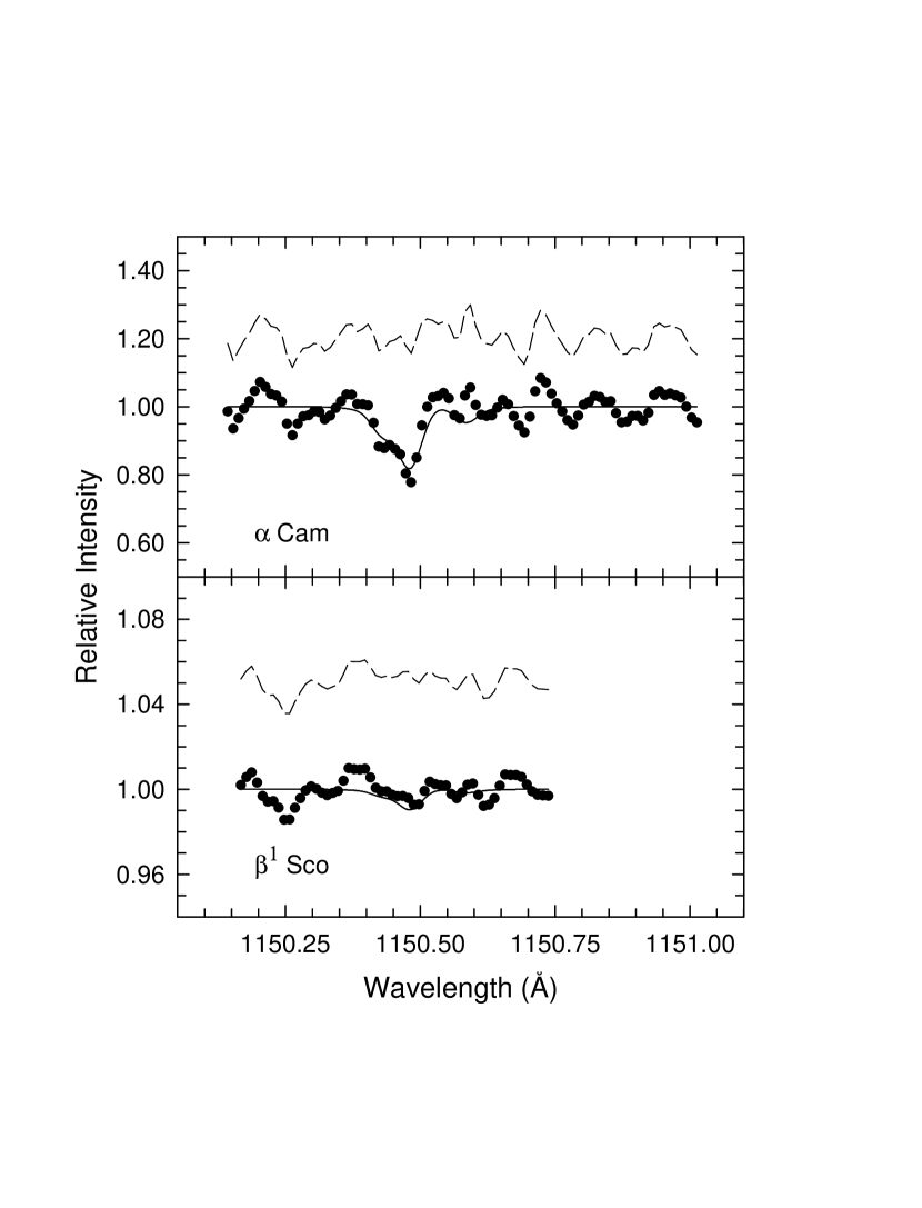
Figure 1: Examples of fits to the $B-X$ bands in spectra for $\alpha$ Cam (upper panel) and $\beta^{1}$ Sco (lower panel). The data are represented by filled circles, and the fit from the profile synthesis is the solid line through the data points. The dashed line shows the difference between fit and data, offset to 1.20 and 1.05 in the spectrum for $\alpha$ Cam and $\beta^{1}$ Sco, respectively. The spectrum for $\beta^{1}$ Sco, which is shown on an expanded vertical scale, yields an upper limit to the amount of CO absorption.

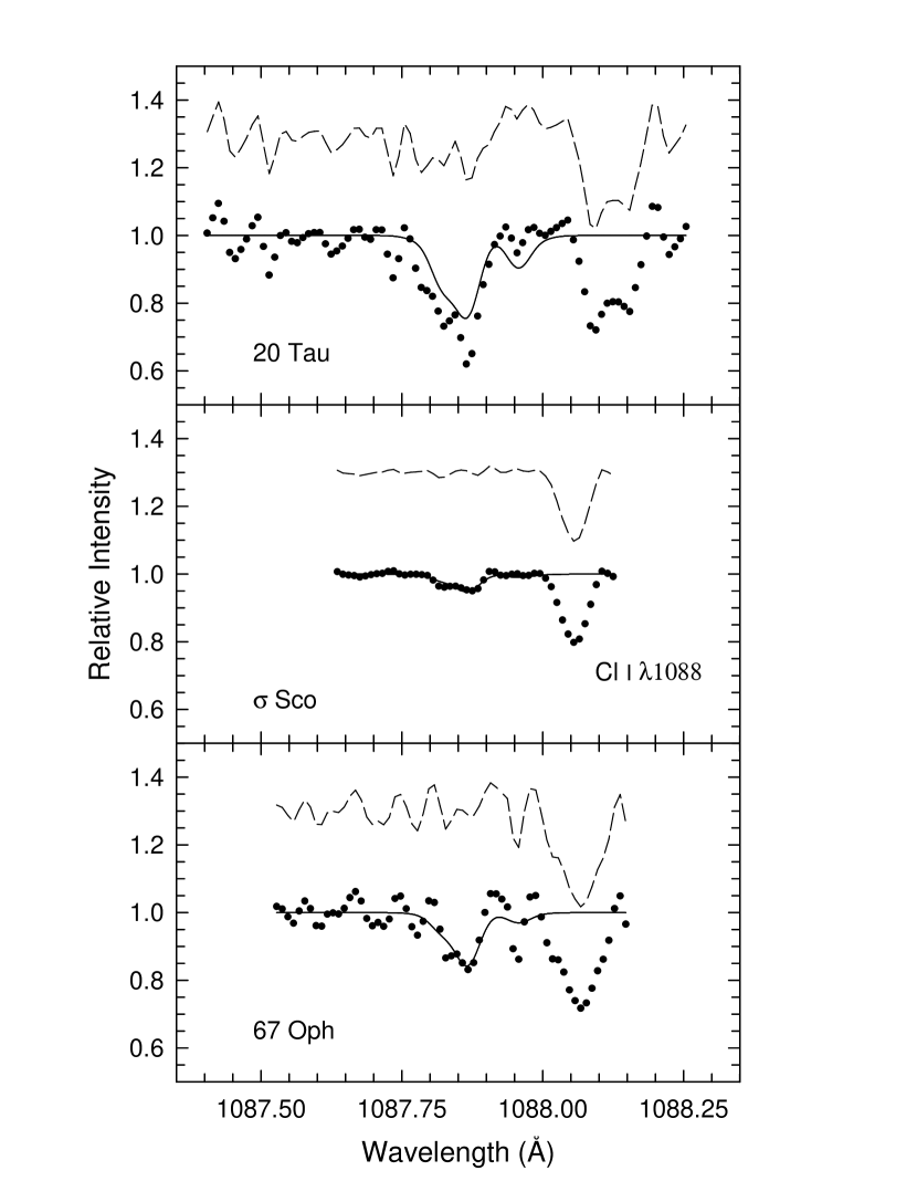
Figure 2: Same as Fig. 1 for $C-X$ bands seen toward 20 Tau (upper panel), $\sigma$ Sco (middle panel), and 67 Oph (lower panel). Here, the fit-data is offset to 1.30 in all panels. The feature near 1088.05 Å is a line from Cl I.

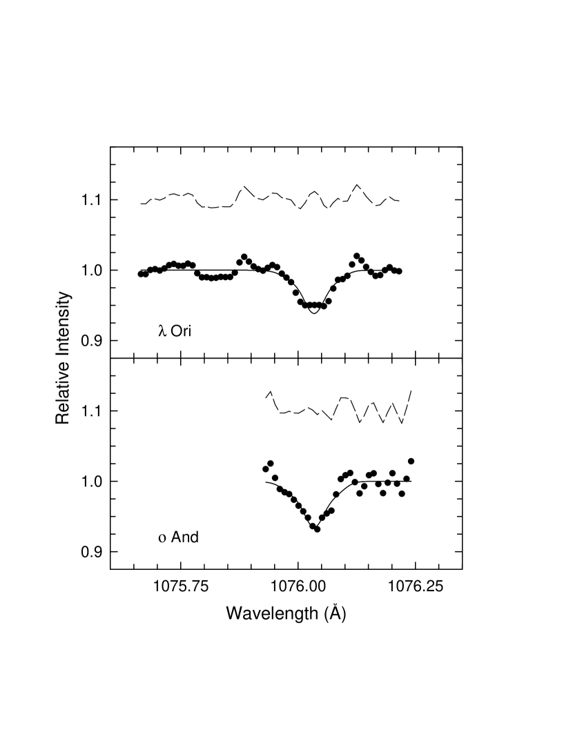
Figure 3: Same as Fig. 1 for the $E-X$ bands at 1076 Å seen toward $\lambda$ Ori (upper panel) and $o$ And (lower panel). Here, the offset for fit-data is 1.10.

We extracted high-resolution spectra taken with the U1 photomultiplier tube from the $Copernicus$ archive at the Multiwavelength Archive at the Space Telescope Science Institute. The nominal spectral resolution was 0.05 Å. The spectra covered absorption from the $B-X$ (0-0) band at 1150 Å, the $C-X$ (0-0) band at 1088 Å, and the $E-X$ (0-0) band at 1076 Å. Individual scans were examined; those completely encompassing the CO band and free from peculiarities were rebinned and summed to yield a final spectrum. The stellar continua were fitted with a low-order polynomial within the IRAF environment to produce rectified spectra for further analysis. Examples of rectified spectra are shown in Figures 1 to 3. There are two points to note about these spectra. First, the available spectral range was limited by the coverage of the spectral scan. This is evident in the $o$ And spectrum near the $E-X$ band (see Fig. 3). Second, a chlorine line at 1088 Å is the feature at longer wavelengths in Fig. 2.

Equivalent widths ($W_{\lambda}$) were measured off these spectra for comparison with earlier work and with our results of fitting the CO band profiles. The values of $W_{\lambda}$ appear in Table 1; upper limits represent 3-$\sigma$ values. The quoted uncertainties were determined from the root-mean-square (rms) deviations in the stellar continuum and the width of the feature at the 50% level. For upper limits, the width was taken to be 0.05 Å or the apparent value for a 2-$\sigma$ ‘feature’, whichever was larger.

There are three potential sources of background in coadded $Copernicus$ spectra, energetic particle counts, stray light, and scattered light. All archived spectra were corrected for particle background. Procedures to eliminate stray light were introduced in data acquired after 19 April, 1973. For measurements before this date, we estimated the contribution from stray light by examining scans of saturated H₂ and N II lines at nearby wavelengths. In the worst cases (HD 21278, 67 Oph, and $o$ And), about 30% of the continuum level could be from stray light. Since accidental blockage of the stray light source could have taken place in the CO scans, we did not apply any corrections, but instead note the three sight lines by different symbols in the plots described below. Neither did we correct for scattered light, which could represent 5 to 10% of the local continuum.

As note above, many of these spectra were analyzed by others. For most bands, the earlier measurements of $W_{\lambda}$ (Morton & Hu 1975; Federman et al. 1980) and ours show relatively good agreement, consistent at the 2-$\sigma$ level. Essentially all are consistent at the quoted 3-$\sigma$ level. The results for $\sigma$ Sco may agree as well, but we note that Allen et al. (1990) did not provide an estimate for the uncertainty in their measurement. The main difference is that our results generally have smaller uncertainties because (1) all available data were used to produce final spectra and (2) the rms deviations in the stellar continua were more easy to quantify upon adoption of low-order polynomials for their shapes. Our values for $W_{\lambda}$ tend to be smaller than earlier measures; this may also be due to our ability for improved fits to stellar continua. Since Snow & Jenkins (1980) only presented column densities obtained from fitting the CO band profiles, we compare their results with ours after describing our method for profile synthesis.

Each band was synthesized separately with the least-squares fitting routine (see Lambert et al. 1994) used in our laboratory study of Rydberg transitions (Federman et al. 2001). The wavelengths for individual rotational lines were taken from the compilation of Eidelsberg et al. (1991), and we used the $f$-values of Federman et al. (2001) for the $B-X$ (0-0), $C-X$ (0-0), and $E-X$ (0-0) bands seen in our spectra. Moreover, a $b$-value of 1 km s^-1, based on ultra-high-resolution studies ($\lambda$/$\delta\lambda$ $=$ 500,000 to 900,000) of CH absorption in diffuse clouds (Crane, Lambert, & Sheffer 1995; Crawford 1995), and an instrumental width of 0.05 Å were adopted. [A similar value of 1.2 km s^-1 was adopted by Snow & Jenkins (1980) in their study of sight lines in Scorpius.] For each spectrum, the wavelength offset for the R(0) line and column density were varied until the difference between measured and synthesized spectra was minimized. (The spectra shown in Fig. 1-3 have the R(0) line appearing at its laboratory wavelength.) As indicated by the values of $W_{\lambda}$ in Table 1, the absorption is quite weak in most instances. Only in the cases of stronger absorption can one discern partially resolved rotational structure. For spectra revealing stronger absorption (e.g., see Fig. 2), we were able to infer the rotational excitation temperature ($T_{ex}$) as well. This was done in an iterative manner; for sight lines revealing absorption from more than one band, comparison of fitting results among bands was performed. Otherwise, $T_{ex}$ was set at 4.0 K. For many of the directions, more than one neutral gas component is seen in C I spectra taken with the Goddard High Resolution Spectrograph (GHRS) on the Hubble Space Telescope (Zsargó & Federman 2003). Since these directions tend to have rather weak CO absorption, the inferred CO column densities are not especially sensitive to optical depth effects, regardless of the number of components or the adopted $b$-value. For example, a column density of $3\times 10^{13}$ cm^-2, larger than found for most of the present sample, yields an optical depth at line center of $\approx$ 3 for R(0) in the strong $C-X$ band.

The results of our fits appear in Table 2. The CO column density toward $\epsilon$ Per differs by a small amount ($\leq$ 2%) compared to that analyzed by Zsargó & Federman (2003) and so their conclusions are not altered. The listed uncertainties for individual determinations of column density are based on the uncertainties in $W_{\lambda}$. In cases where fits to more than one band were possible, the final column density was derived by taking a weighted mean of the individual determinations. Fits to spectra showing no clear absorption in one band yielded consistent column densities. However, the column density toward $\lambda$ Ori from the $W_{\lambda}$ for the $B-X$ band clearly is much larger than with those from the other bands and is not listed in Table 2. In a similar vein, the relatively large upper limits determined for the $B-X$ band toward 1 Sco, $\nu$ Sco, $\mu$ Nor, and $\gamma$ Ara are not especially useful. Finally, for sight lines with only upper limits, the most stringent column density was used in our analyses below.

We now compare the results of the fits with our direct measurements for $W_{\lambda}$ and with the column densities given by Snow & Jenkins (1980) and Federman et al. (1994). For the most part, the values of $W_{\lambda}$ derived from profile synthesis agree very well with our new measurements. The largest differences in $W_{\lambda}$, usually at the 2-$\sigma$ level, occur for the $C-X$ band, such as that seen in Fig. 2 for 20 Tau. The band is partially blended with absorption from Cl I at 1088 Å, making these spectra the most susceptible to a poorly defined continuum. The comparison with the column densities of Snow & Jenkins is less satisfactory. Their column densities are several times larger than ours. The difference does not lie in the adopted $b$-value or $T_{ex}$; they are very similar. Moreover, the $f$-values used in the fits, those quoted by Snow (1975) versus those of Federman et al. (2001), are not that different. Other possible causes cannot be discerned because Snow & Jenkins did not tabulate $W_{\lambda}$. Federman et al. (1994) used published values for $W_{\lambda}$ and updated $f$-values for the $C-X$ and $E-X$ bands in their compilation. Differences between their adopted values of $W_{\lambda}$ and our fitted ones, when combined with the factor of 1.6 for the ratio of adopted $f$-values [those of Federman et al. (2001) being larger], successfully explains the differences seen in the present column densities and the ones quoted in the compilation. In passing we note that Federman et al. (1994) also found self-consistent results from the two CO bands because the new and older $f$-values differ by a scale factor (1.6).

2.2 Data from the Hubble Space Telescope

In the course of our study on nonthermal chemistry in gas with low molecular abundances (Zsargó & Federman 2003), we found archival spectra for HD 112244 covering the $A-X$ (4-0) and (5-0) bands. The data were acquired with grating G160M of the GHRS. The spectra (z0yv0607m, z0yv0608m, and z0yv0609m) were reduced in the manner described by Zsargó & Federman. In addition, we smoothed the final, rectified spectra by three pixels to increase the signal to noise. The bands were synthesized with the $f$-values of Chan et al. (1993), a $b$-value of 1 km s^-1, and $T_{ex}$ of 4.0 K. The values for $W_{\lambda}$ and the column densities appear in Table 3. Two components are discerned, though the weaker, bluer one is formally a 2.5-$\sigma$ detection. Its reality is strengthened by the fact that the velocity separation of $\sim$ 25 km s^-1 agrees nicely with those seen in CH (Danks, Federman, & Lambert 1984) and C I (Zsargó & Federman 2003), 24.6 and 24.1 km s^-1, respectively. As found here for CO, the red CH component is the stronger one, while the two components have similar strengths in C I.

3 Discussion

3.1 General Comments

The results described in the last Section represent the lowest CO column densities measured in interstellar space. Most determinations are in the range of $10^{12}$ to $10^{13}$ cm^-2. Studies of CO emission at millimeter wavelengths generally are sensitive to column densities greater than $10^{15}$ cm^-2, values seen in molecule-rich diffuse gas like that toward $\zeta$ Oph (e.g., Lambert et al. 1994). Even when measuring absorption at millimeter wavelengths against background extragalactic sources (e.g., Liszt & Lucas 1998), column densities are found to be greater than $10^{14}$ cm^-2. Clearly, UV absorption is the most sensitive probe of CO in diffuse clouds.

This conclusion is consistent with another result arising from our profile syntheses. We find that the CO excitation temperature is barely above the 2.7 K value of the Cosmic Background. For comparison, $T_{ex}$ is about 4 to 6 K in molecule-rich diffuse gas (e.g., Lambert et al. 1994; Federman et al. 2003). The gas probed by our observations reveal severe subthermal CO excitation, another indication that we are sampling a relatively low density environment. Analysis of C I excitation (Zsargó & Federman 2003) for many of the same directions leads to density estimates of 10 to 200 cm^-3, with the larger estimates associated with sight lines (in Scorpius) having $T_{ex}$ of 4 K. For most of our other sight lines, Jenkins, Jura, & Loewenstein (1983) extracted pressures from C I absorption seen in $Copernicus$ spectra. When combined with the kinetic temperatures deduced from the $J$ $=$ 0 and 1 levels of H₂ (Savage et al. 1977), low densities are again inferred.

3.2 Correlations among Species

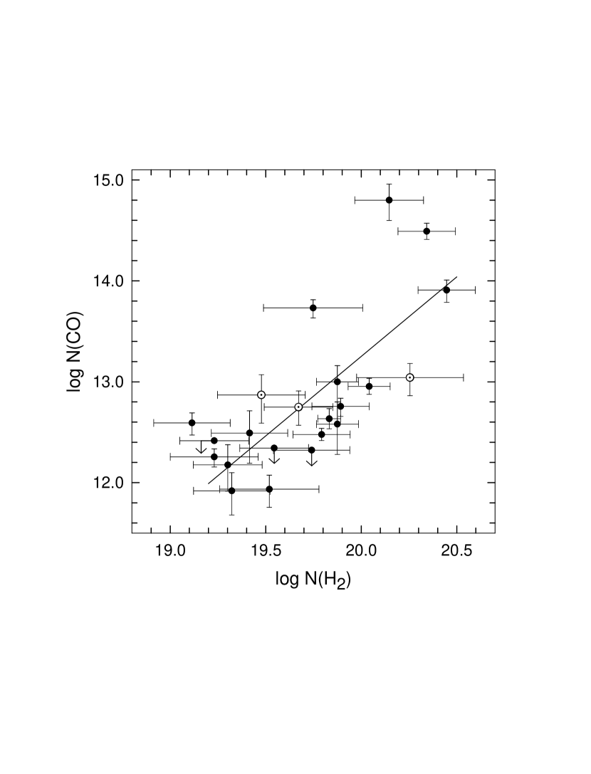
Figure 4: Plot of log $N$(CO) vs. log $N$(H₂) for the sight lines in the present survey. Results for HD 21278, 67 Oph, and $o$ And, where a 30% (0.11 dex) contribution from stray light may be present, are indicated by dotted open circles. The 2-$\sigma$ observational uncertainties are shown. The solid line is the fit from the linear regression analysis with censored data $-$ i.e., upper limits.

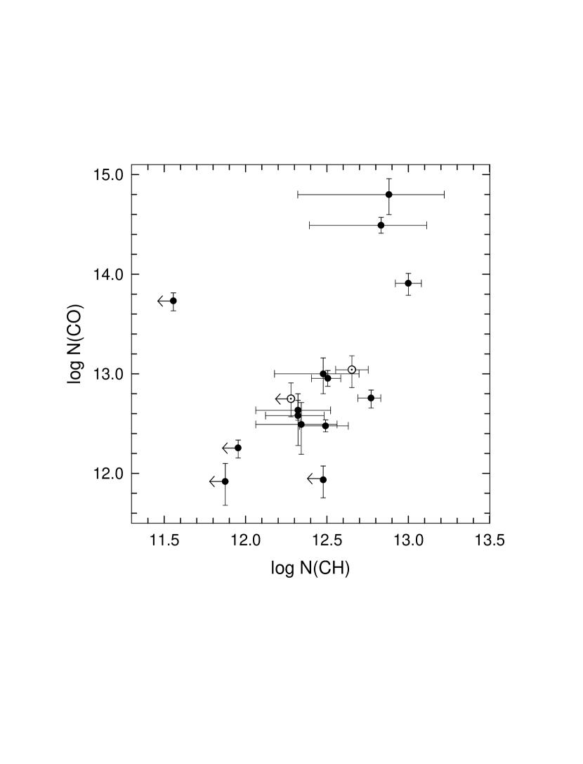
Figure 5: Plot of log $N$(CO) vs. log $N$(CH) for the sight lines in the present survey.

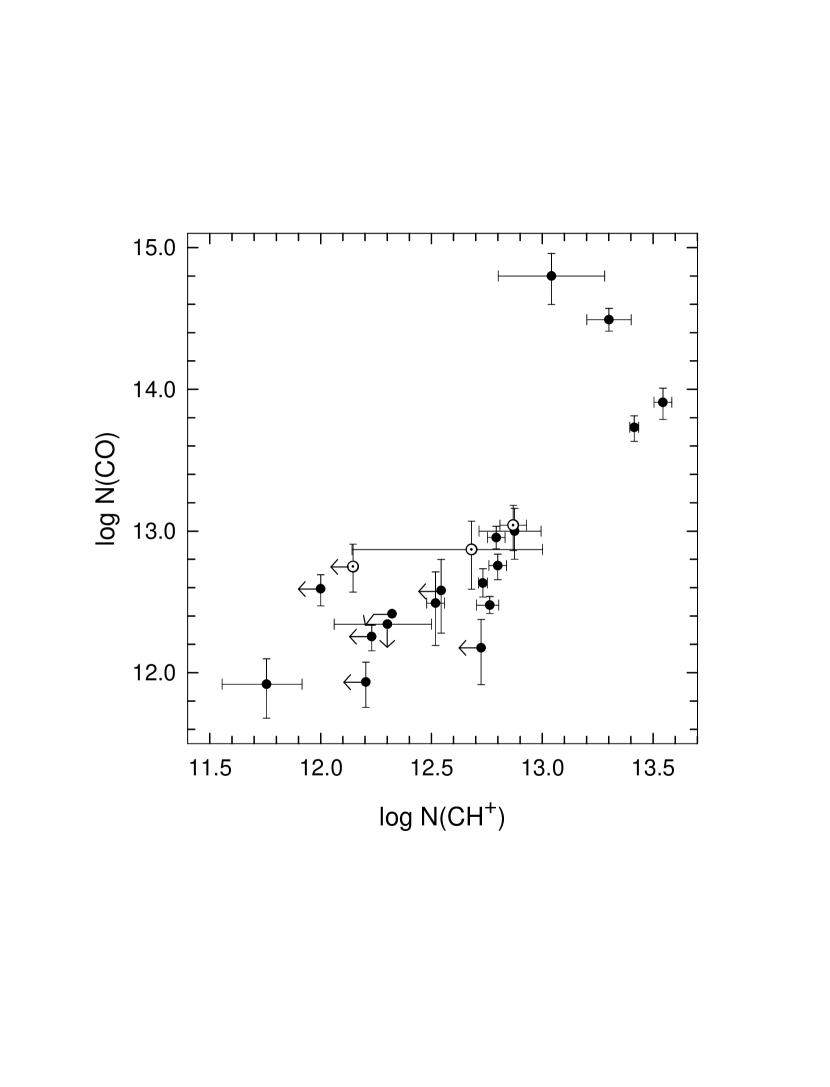
Figure 6: Plot of log $N$(CO) vs. log $N$(CH⁺) for the sight lines in the present survey.

The correspondences between $N$(CO) with $N$(H₂), $N$(CH), and $N$(CH⁺) for our set of directions appear in Figures 4-6. The plots distinguish between components A and B toward HD 112244. The upper limit for $N$(CH⁺) in component B is obtained by multiplying the uncertainty given by Lambert & Danks (1986) for component A by 3. The H₂ column densities come from Savage et al. (1977). The two components toward HD 112244 were given half the total H₂, consistent with the similar amounts of C I in each (Zsargó & Federman 2003). The results for CH come from the compilation of Federman et al. (1994), updated to include the column densities found by Crane et al. (1995), and those for CH⁺ are from Federman (1982), Lambert & Danks (1986), Crane et al. (1995), and Price et al. (2001). The column densities used in this analysis appear in Table 4. Typical uncertainities are 30% for $N$(H₂) and 10 to 30% for the column densities of carbon-bearing molecules. We adopted 3-$\sigma$ upper limits for non-detections.

The relationship involving CO and H₂ appears to show a reasonable correlation. If we assume the upper limits are detections, the correlation coefficient ($r^{2}$) is 0.53. Since our set of data includes upper limits on CO, we also performed a linear regression with censored data, relying on the package ASURV-Rev. 1.1 (see Isobe, Feigelson, & Nelson 1986; Isobe & Feigelson 1990; La Valley, Isobe, & Feigelson 1992). The Buckley-Jones method was employed because limits existed only for the dependent variable, log $N$(CO). The fit is shown in Fig. 4 as the solid line; the slope is $1.58\pm 0.34$ and the intercept is $-$18.35. The fitted results are nearly identical to those from a simple linear least-squares fit ($1.46\pm 0.31$ and $-$16.0) because few data are represented by limits. The slope is similar to the one found previously by Federman et al. (1980), whose survey included both molecule-rich and molecule-poor lines of sight.

The value of the slope arises from the competition between CO production under equilibrium conditions in colder, denser gas ($n$ $\gtrsim 100$ cm^-3) and production as a result of CH⁺ synthesis in lower density gas ($n$ $\lesssim 100$ cm^-3). Under equilibrium conditions in diffuse molecular clouds, CO is a second generation molecule, forming in appreciable quantities once significant amounts of OH are present (e.g., Federman & Huntress 1989). In particular, the synthesis of CO mainly arises from reactions between C⁺ and OH. If this were the only pathway leading to CO, a slope of 2 would be expected (Federman et al. 1984). On the other hand, when CH⁺ is synthesized in lower density material in the cloud via nonequilibrium processes, observable amounts of CO are produced in subsequent reactions involving CH⁺ and O (e.g., Zsargó & Federman 2003). Then $N$(CO) is not dependent on $N$(H₂). The combination of the two schemes leads to a slope smaller than 2. Some of the dispersion seen in Fig. 4 probably results from differences in the relative contributions from the two pathways for CO. For directions in common with the present study, Zsargó & Federman typically find 10 to 30% of the CO comes from CH⁺, except for the sight lines in Scorpius where most of the CO is attributed to the presence of CH⁺ because the densities are several times higher. Moreover, the modest relationship between CO and H₂ likely arises because most of the H₂ along the line of sight is associated with the denser material, not the gas containing CH⁺.

Since there is a strong correlation between log $N$(CH) and log $N$(H₂) in diffuse molecular gas (Federman 1982; Danks et al. 1984), it is surprising at first glance to see such a poor correspondence between $N$(CO) and $N$(CH) (Fig. 5), where $r^{2}$ $=$ 0.21. The correlation coefficient of 0.54 for log $N$(CH) versus log $N$(H₂) for our dataset indicates a tighter correspondence, but even this is significantly less than $r^{2}$ $=$ 0.80 found by Danks et al. While a linear regression by the Schmitt Method in ASURV (which treats limits in the independent variable) suggests that 4 of 5 upper limits are consistent with detections, the slope and intercept are not well defined. The relationship also contrasts with the one revealed in Fig. 9 of Federman et al. (1994). The key to understanding the present result lies in the source for CH in our sample. The sight lines in the current survey are not particularly rich in molecules in large part because the gas densities are rather low (e.g., Zsargó & Federman 2003). Confirmation of low densities comes from observations of C₂ and CN, tracers of denser gas (Joseph et al. 1986; Federman et al. 1994), which yield only upper limits for the sight lines examined here. Zsargo & Federman found that most of the observed CH could be attributed to production of CH⁺ under nonequilibrium conditions. (Like CO, CH is produced under both equilibrium and nonequilibrium conditions.) Since reactions between CH and O play a minor role compared to those between CH⁺ and O (Zsargó & Federman 2003), little correspondence between CO and CH is expected for our sight lines. On the other hand, the sample in Federman et al. (1994) primarily contains molecule-rich clouds where CH chemistry is intimately tied to the amount of H₂ (Federman 1982; Danks et al. 1984).

The data in Fig. 6 suggest a correlation between CO and CH⁺ as well ($r^{2}$ $=$ 0.61 assuming all data are detections). The slope is $1.31\pm 0.24$, yet a linear relationship is expected when CO arises from CH⁺ $+$ O (Federman et al. 1984). The Schmitt Method indicates that only 2 of 8 upper limits are possible detections and yields a slope that is not well determined. Therefore, it seems that the apparent correlation is strongly influenced by the results for $\pi$ Sco in the lower left corner of the plot. Most of the CO appears to exist in regions denser than those responsible for the CH⁺ (and CH) toward many stars in our sample.

In summary, we presented the most complete, internally consistent set of CO column densities for sight lines containing modest amounts of molecular material. These column densities are relatively small; CO self-shielding does not affect the photodissociation rate needed to model these sight lines. Thus our results can be used to test chemical aspects of the models that do not rely on radiative transfer in lines. The correspondence between CO and H₂ found in earlier studies is still present, but there is no apparent connection with CH for these directions. This latter result indicates that much of the CO is probing the denser portions of our sample of diffuse clouds, those clouds where CH is mainly produced as a by-product of CH⁺ synthesis. The ambiguous relationship between CO and CH⁺ also seems to reflect different chemical environments.

Table 1: CO Measurements with the $Copernicus$ Satellite

		$W_{\lambda}$ (mÅ)
HD	Star	$B-X$ (1150 Å)				$C-X$ (1088 Å)				$E-X$ (1076 Å)
		Measured	Fit	Other		Measured	Fit	Other		Measured	Fit	Other
21278		$\ldots$	$\ldots$	$\ldots$		8.6$\pm$2.3	11.1	21$\pm$3 a		2.5$\pm$0.8	5.3	7$\pm$5 a
23408	20 Tau	$\ldots$	$\ldots$	$\ldots$		31.1$\pm$3.6	25.9	32$\pm$8 a		$\ldots$	$\ldots$	$\ldots$
23630	$\eta$ Tau	$\ldots$	$\ldots$	$\ldots$		$\leq$ 4.1	$\leq$ 3.2	2.8$\pm$2.4 a		$\ldots$	$\ldots$	$\ldots$
24760	$\epsilon$ Per	$\ldots$	$\ldots$	$\ldots$		1.4$\pm$0.3	1.4	8$\pm$2 a		0.6$\pm$0.2	0.7	1.3$\pm$0.7 a
30614	$\alpha$ Cam	12.9$\pm$2.6	16.8	$\ldots$		67.6$\pm$6.0	46.4	44 b		$\ldots$	$\ldots$	$\ldots$
36861	$\lambda$ Ori	1.9$\pm$0.2	$\ldots$	$\ldots$		3.9$\pm$0.7	4.7	24 b		4.6$\pm$0.8	4.6	$\ldots$
40111	139 Tau	$\ldots$	$\ldots$	$\ldots$		$\leq$ 2.8	$\leq$ 3.1	4.0$\pm$2.8 a		$\ldots$	$\ldots$	$\ldots$
141637	1 Sco	$\leq$ 11.0	$\ldots$	$\ldots$		$\leq$ 3.8	$\leq$ 3.8	$\ldots$		$\ldots$	$\ldots$	$\ldots$
143018	$\pi$ Sco	$\ldots$	$\ldots$	$\ldots$		0.8$\pm$0.2	1.3	0.8$\pm$0.2 a		$\ldots$	$\ldots$	$\ldots$
143275	$\delta$ Sco	$\ldots$	$\ldots$	$\ldots$		3.6$\pm$1.1	4.5	6.0$\pm$0.8 a, c		$\ldots$	$\ldots$	$\ldots$
144217	$\beta^{1}$ Sco	$\leq$ 1.5	$\leq$ 0.8	$\ldots$		5.4$\pm$0.6	6.0	c		$\ldots$	$\ldots$	$\ldots$
144470	$\omega^{1}$ Sco	1.1$\pm$0.2	1.0	c		8.5$\pm$0.9	10.4	12$\pm$1.6 a, c		$\ldots$	$\ldots$	$\ldots$
145502	$\nu$ Sco	$\leq$ 6.1	$\ldots$	$\ldots$		5.9$\pm$0.6	7.5	5.0$\pm$2.2 a, c		$\ldots$	$\ldots$	$\ldots$
147165	$\sigma$ Sco	$\ldots$	$\ldots$	$\ldots$		3.7$\pm$0.3	4.4	6 d		$\ldots$	$\ldots$	$\ldots$
149038	$\mu$ Nor	$\leq$ 17.0	$\ldots$	$\ldots$		30.7$\pm$3.8	30.2	39$\pm$7 a		$\ldots$	$\ldots$	$\ldots$
157246	$\gamma$ Ara	$\leq$ 3.6	$\ldots$	$\ldots$		2.1$\pm$0.2	2.6	3.2$\pm$0.8 e		1.6$\pm$0.3	1.7	2.6$\pm$0.7 e
164353	67 Oph	$\ldots$	$\ldots$	$\ldots$		13.0$\pm$2.1	12.9	10$\pm$7 a		6.7$\pm$1.2	6.3	8$\pm$4 a
200120	59 Cyg	$\ldots$	$\ldots$	$\ldots$		1.5$\pm$0.4	2.3	5.0$\pm$1.5 a		$\leq$ 1.1	$\leq$ 0.9	0.9$\pm$1.4 a
217675	$o$ And	$\ldots$	$\ldots$	$\ldots$		5.1$\pm$0.7	6.4	12$\pm$2 a		4.8$\pm$1.2	5.1	10$\pm$3 a
218376	1 Cas	$\ldots$	$\ldots$	$\ldots$		58.7$\pm$12.0	52.7	$\ldots$		$\ldots$	$\ldots$	$\ldots$

Table 2: Results of Profile Synthesis ^a

Star	$N$(CO) (cm-2)				$T_{ex}$ (K)
	$B-X$	$C-X$	$E-X$	Final
HD 21278	$\ldots$	$(9.6\pm 5.1)\times 10^{12}$	$(7.0\pm 2.2)\times 10^{12}$	$(7.4\pm 2.0)\times 10^{12}$	4.0
20 Tau	$\ldots$	$(5.4\pm 0.6)\times 10^{13}$	$\ldots$	$(5.4\pm 0.6)\times 10^{13}$	3.0
$\eta$ Tau	$\ldots$	$\leq$ $2.2\times 10^{12}$	$\ldots$	$\leq$ $2.2\times 10^{12}$	4.0
$\epsilon$ Per	$\ldots$	$(8.8\pm 1.9)\times 10^{11}$	$(8.1\pm 2.7)\times 10^{11}$	$(8.6\pm 1.6)\times 10^{11}$	3.0
$\alpha$ Cam	$(3.1\pm 0.6)\times 10^{14}$	$(3.1\pm 0.3)\times 10^{14}$	$\ldots$	$(3.1\pm 0.3)\times 10^{14}$	3.3
$\lambda$ Ori	b	$(3.2\pm 0.6)\times 10^{12}$	$(5.8\pm 1.0)\times 10^{12}$	$(3.9\pm 0.5)\times 10^{12}$	3.2
139 Tau	$\ldots$	$\leq$ $2.1\times 10^{12}$	$\ldots$	$\leq$ $2.1\times 10^{12}$	4.0
1 Sco	b	$\leq$ $2.6\times 10^{12}$	$\ldots$	$\leq$ $2.6\times 10^{12}$	4.0
$\pi$ Sco	$\ldots$	$(8.3\pm 2.0)\times 10^{11}$	$\ldots$	$(8.3\pm 2.0)\times 10^{11}$	4.0
$\delta$ Sco	$\ldots$	$(3.1\pm 0.9)\times 10^{12}$	$\ldots$	$(3.1\pm 0.9)\times 10^{12}$	4.0
$\beta^{1}$ Sco	$\leq$ $8.1\times 10^{12}$	$(4.3\pm 0.5)\times 10^{12}$	$\ldots$	$(4.3\pm 0.5)\times 10^{12}$	4.0
$\omega^{1}$ Sco	$(10.0\pm 2.0)\times 10^{12}$	$(8.8\pm 1.0)\times 10^{12}$	$\ldots$	$(9.0\pm 0.9)\times 10^{12}$	4.0
$\nu$ Sco	b	$(5.7\pm 0.6)\times 10^{12}$	$\ldots$	$(5.7\pm 0.6)\times 10^{12}$	3.2
$\sigma$ Sco	$\ldots$	$(3.0\pm 0.2)\times 10^{12}$	$\ldots$	$(3.0\pm 0.2)\times 10^{12}$	4.0
$\mu$ Nor	b	$(8.1\pm 1.0)\times 10^{13}$	$\ldots$	$(8.1\pm 1.0)\times 10^{13}$	3.0
$\gamma$ Ara	b	$(1.7\pm 0.2)\times 10^{12}$	$(2.0\pm 0.4)\times 10^{12}$	$(1.8\pm 0.2)\times 10^{12}$	3.2
67 Oph	$\ldots$	$(1.3\pm 0.2)\times 10^{13}$	$(0.8\pm 0.3)\times 10^{13}$	$(1.1\pm 0.2)\times 10^{13}$	3.0
59 Cyg	$\ldots$	$(1.5\pm 0.4)\times 10^{12}$	$\leq$ $1.1\times 10^{12}$	$(1.5\pm 0.4)\times 10^{12}$	3.0
$o$ And	$\ldots$	$(4.7\pm 1.6)\times 10^{12}$	$(6.6\pm 1.6)\times 10^{12}$	$(5.6\pm 1.1)\times 10^{12}$	3.5
1 Cas	$\ldots$	$(6.3\pm 1.3)\times 10^{14}$	$\ldots$	$(6.3\pm 1.3)\times 10^{14}$	3.0

Table 3: Results for HD 112244

Component	$A-X$ (4-0)				$A-X$ (5-0)
	$W_{\lambda}$(obs)	$W_{\lambda}$(fit)	$N$(CO) a		$W_{\lambda}$(obs)	$W_{\lambda}$(fit)	$N$(CO) a
	(mÅ)	(mÅ)	(cm-2)		(mÅ)	(mÅ)	(cm-2)
A b	3.9$\pm$0.7	4.3	$(1.1\pm 0.2)\times 10^{13}$		1.9$\pm$0.6	2.2	$(0.9\pm 0.3)\times 10^{13}$
B	1.2$\pm$0.5	1.2	$(3.0\pm 1.3)\times 10^{12}$		1.6$\pm$0.6	1.6	$(6.4\pm 2.4)\times 10^{12}$

Table 4: Molecular Column Densities

Star	$N$(CO)	$N$(H2)	$N$(CH)	$N$(CH+)
	(cm-2)	(cm-2)	(cm-2)	(cm-2)
HD 21278	$7.4\times 10^{12}$	$3.0\times 10^{19}$	$\ldots$	$4.8\times 10^{12}$
20 Tau	$5.4\times 10^{13}$	$5.6\times 10^{19}$	$\leq$ $3.6\times 10^{11}$	$2.6\times 10^{13}$
$\eta$ Tau	$\leq$ $2.2\times 10^{12}$	$3.5\times 10^{19}$	$\ldots$	$2.0\times 10^{12}$
$\epsilon$ Per	$8.6\times 10^{11}$	$3.3\times 10^{19}$	$\leq$ $3.0\times 10^{12}$	$\leq$ $1.6\times 10^{12}$
$\alpha$ Cam	$3.1\times 10^{14}$	$2.2\times 10^{20}$	$6.8\times 10^{12}$	$2.0\times 10^{13}$
$\lambda$ Ori	$3.9\times 10^{12}$	$1.3\times 10^{19}$	$\ldots$	$\leq$ $1.0\times 10^{12}$
139 Tau	$\leq$ $2.1\times 10^{12}$	$5.5\times 10^{19}$	$\ldots$	$\ldots$
HD 112244A a	$1.0\times 10^{13}$	$7.5\times 10^{19}$	$3.0\times 10^{12}$	$7.5\times 10^{12}$
HD 112244B a	$3.8\times 10^{12}$	$7.5\times 10^{19}$	$2.1\times 10^{12}$	$\leq$ $3.5\times 10^{12}$
1 Sco	$\leq$ $2.6\times 10^{12}$	$1.7\times 10^{19}$	$\ldots$	$\leq$ $2.1\times 10^{12}$
$\pi$ Sco	$8.3\times 10^{11}$	$2.1\times 10^{19}$	$\leq$ $7.5\times 10^{11}$	$5.7\times 10^{11}$
$\delta$ Sco	$3.1\times 10^{12}$	$2.6\times 10^{19}$	$2.2\times 10^{12}$	$3.3\times 10^{12}$
$\beta^{1}$ Sco	$4.3\times 10^{12}$	$6.8\times 10^{19}$	$2.1\times 10^{12}$	$5.4\times 10^{12}$
$\omega^{1}$ Sco	$9.0\times 10^{12}$	$1.1\times 10^{20}$	$3.2\times 10^{12}$	$6.2\times 10^{12}$
$\nu$ Sco	$5.7\times 10^{12}$	$7.8\times 10^{19}$	$5.9\times 10^{12}$	$6.3\times 10^{12}$
$\sigma$ Sco	$3.0\times 10^{12}$	$6.2\times 10^{19}$	$3.1\times 10^{12}$	$5.8\times 10^{12}$
$\mu$ Nor	$8.1\times 10^{13}$	$2.8\times 10^{20}$	$1.0\times 10^{13}$	$3.5\times 10^{13}$
$\gamma$ Ara	$1.8\times 10^{12}$	$1.7\times 10^{19}$	$\leq$ $9.0\times 10^{11}$	$\leq$ $1.7\times 10^{12}$
67 Oph	$1.1\times 10^{13}$	$1.8\times 10^{20}$	$4.5\times 10^{12}$	$7.4\times 10^{12}$
59 Cyg	$1.5\times 10^{12}$	$2.0\times 10^{19}$	$\ldots$	$\leq$ $5.3\times 10^{12}$
$o$ And	$5.6\times 10^{12}$	$4.7\times 10^{19}$	$\leq$ $1.9\times 10^{12}$	$\leq$ $1.4\times 10^{12}$
1 Cas	$6.3\times 10^{14}$	$1.4\times 10^{20}$	$7.6\times 10^{12}$	$1.1\times 10^{13}$

References

- Allen, Snow, & Jenkins (1990) Allen, M.M., Snow, T.P., & Jenkins, E.B. 1990, ApJ, 355, 130
- Chan, Cooper, & Brion (1993) Chan, W.F., Cooper, G., & Brion, C.E. 1993, Chem. Phys., 170, 123
- Crane, Lambert, & Sheffer (1995) Crane, P., Lambert, D.L., & Sheffer, Y. 1995, ApJS, 99, 107
- Crawford (1995) Crawford, I.A. 1995, MNRAS, 277, 458
- Danks, Federman, & Lambert (1984) Danks, A.C., Federman, S.R., & Lambert D.L. 1984, A&A, 130, 62
- Draine & Katz (1986) Draine, B.T., & Katz, N. 1986, ApJ, 306, 655
- Eidelsberg et al. (1991) Eidelsberg, M., Benayuon, J.J., Viala, Y., & Rostas, F. 1991, A&AS, 90, 231
- Eidelsberg et al. (1999) Eidelsberg, M., Jolly, A., Lemaire, J.L., Tchang-Brillet, W.-Ü. L., Breton, J., & Rostas, F. 1999, A&A, 346, 705
- Federman (1982) Federman, S.R. 1982, ApJ, 257, 125
- Federman et al. (1984) Federman, S.R., Danks, A.C., & Lambert, D.L. 1984, ApJ, 287, 219
- Federman et al. (2001) Federman, S.R., Fritts, M., Cheng, S., Menningen, K.L., Knauth, D.C., & Fulk, K. 2001, ApJS, 134, 133
- Federman et al. (1980) Federman, S.R., Glassgold, A.E., Jenkins, E.B., & Shaya, E.J. 1980, ApJ, 242, 545
- Federman & Huntress (1989) Federman, S.R., & Huntress, W.T. 1989, ApJ, 338, 140
- Federman et al. (2003) Federman, S.R., Lambert, D.L., Sheffer, Y., Cardelli, J.A., Andersson, B.-G., van Dishoeck, E.F., & Zsargó, J. 2003, ApJ, 591, 986
- Federman et al. (1994) Federman, S.R., Strom, C.J., Lambert, D.L., Cardelli, J.A., Smith, V.V., & Joseph, C.L. 1994, ApJ, 424, 772
- Isobe & Feigelson (1990) Isobe, T., & Feigelson, E.D. 1990, BAAS, 22, 917
- Isobe, Feigelson, & Nelson (1986) Isobe, T., Feigelson, E.D., & Nelson, P.I. 1986, ApJ, 306, 490
- Jenkins et al. (1973) Jenkins, E.B., Drake, J.F., Morton, D.C., Rogerson, J.B., Spitzer, L., & York, D.G. 1973, ApJ, 181, L122
- Jenkins, Jura, & Loewenstein (1983) Jenkins, E.B., Jura, M., & Loewenstein, M. 1983, ApJ, 270, 88
- Joseph et al. (1986) Joseph, C.L., Snow, T.P., Seab, C.G., & Crutcher, R.M. 1986, ApJ, 309, 771
- Lambert & Danks (1986) Lambert, D.L., & Danks, A.C. 1986, ApJ, 303, 401
- Lambert et al. (1994) Lambert, D.L., Sheffer, Y., Gilliland, R.L., & Federman, S.R. 1994, ApJ, 420, 756
- La Valley, Isobe, & Feigelson (1992) La Valley, M., Isobe, T., & Feigelson, E.D. 1992, BAAS, 24, 839
- Liszt & Lucas (1998) Liszt, H.S., & Lucas, R. 1998, A&A, 339, 561
- Morton & Hu (1975) Morton, D.C., & Hu, E. 1975, ApJ, 202, 638
- Price et al. (2001) Price, R.J., Crawford, I.A., Barlow, M.J., & Howrath, I.D. 2001, MNRAS, 328, 555
- Savage et al. (1977) Savage, B.D., Bohlin, R.C., Drake, J.F., & Budich, W. 1977, ApJ, 216, 291
- Snow (1975) Snow, T.P. 1975, ApJ, 201, L21
- Snow & Jenkins (1980) Snow, T.P., & Jenkins, E.B. 1980, ApJ, 241, 161
- van Dishoeck & Black (1988) van Dishoeck, E.F., & Black, J.H., 1988, ApJ, 334, 771
- Zsargó & Federman (2003) Zsargó, J., & Federman, S.R. 2003, ApJ, 589, 319