A Deep, Wide Field, Optical, And Near Infrared Catalog Of A Large Area Around The Hubble Deep Field North¹

Abstract

We have conducted a deep multi-color imaging survey of 0.2 degrees² centered on the Hubble Deep Field North (HDF-N). We shall refer to this region as the Hawaii-HDF-N. Deep data were collected in $U$, $B$, $V$, $R$, $I$, and $z^{\prime}$ bands over the central 0.2 degrees² and in $HK^{\prime}$ over a smaller region covering the Chandra Deep Field North (CDF-N). The data were reduced to have accurate relative photometry and astrometry across the entire field to facilitate photometric redshifts and spectroscopic followup. We have compiled a catalog of 48,858 objects in the central 0.2 degrees² detected at $5\sigma$ significance in a 3^′′ aperture in either $R$ or $z^{\prime}$ band. Number counts and color-magnitude diagrams are presented and shown to be consistent with previous observations. Using color selection we have measured the density of objects at $3<z<7$. Our multi-color data indicates that samples selected at $z>5.5$ using the Lyman break technique suffer from more contamination by low redshift objects than suggested by previous studies.

1 Introduction

Deep surveys provide numerous constraints on the structure and evolution of the universe. It has been known that galaxy number counts in a specific bandpass can provide a useful constraint on galaxy evolution (Tinsley, 1972; Brown & Tinsley, 1974; Tinsley, 1980). Multi-color surveys further constrain the galaxy formation history and allow for the selection of galaxies in specific redshift ranges. This work was pioneered in the Hawaii surveys (Cowie, 1988) and subsequently used extensively by Steidel et. al (Steidel et al., 1996, 1999) for mapping $z\simeq 3$ and $z\simeq 4$ galaxies. By using a color selection these groups were able to select and obtain spectra for over 1000 $z\simeq 3$ galaxies with a 90% success rate. This gave us a wealth of information about this redshift range. With the ability of modern detectors to take deep images in the near IR we can now select galaxies up to $z>6.5$ (Hu et al., 2002). The Hubble Deep Fields (HDFs) (Williams et al., 1996) showed the value of photometric redshifts applied to deep multi-color surveys. This technique allows estimates of redshifts for objects much too faint for optical spectroscopy. It allows for economical measurement of the redshifts of millions of galaxies.

Despite the depth and accuracy of the HDF data, it only covers a small co-moving volume. Postman et al. (1998) have looked at the clustering of galaxies using the two point correlation function of galaxies projected on the sky. This work covered 16 sq. degrees in $I$ band. It has shown that galaxies are highly clustered on scales of 15-20 $h^{-1}$ Mpc where $h=$ Ho/100 km s^-1Mpc^-1. This has provided a challenge in obtaining an unbiased sample of galaxies, since several square degrees must be surveyed. The present paper is the first of a series which will aim to obtain the required data by imaging several 0.2 sq. degree fields.

Previous studies of galaxy formation and evolution have solely used optical data which introduced biases. However new generations of radio, X-ray, and mid-IR telescopes have opened up these wavelengths to deep wide-field surveys. X-rays have constrained the Active Galactic Nuclei (AGN) history (Barger et al., 2002), while radio and mid-IR fluxes have proven to be a good probe of star formation. Space based optical imaging also allowed for the morphological study of galaxies out to high redshift. As such we have chosen to target regions of the sky that have been observed in multiple wave bands. We began with the HDF-N because of its deep and complete multi-wavelength data provided by the Great Observatories Origins Deep Survey (GOODS) and other surveys. We have covered 0.4 square degrees centered on the HDF-N. The central 0.2 square degrees of this data are of consistent quality in all optical bands, this area contains 48,858 objects detected at 5$\sigma$ in $R$ or $z^{\prime}$ band.

This paper is one in a series focusing on the Hawaii HDF-N. The properties of X-ray selected objects are discussed in Barger et al. (2003, 2002). Photometric redshifts, spectroscopic redshifts, and multi-wavelength analysis will be discussed in Capak et al. (2003). The main focus of the present paper is the optical/IR data reduction and catalog. We also provide number counts and color-color plots to allow for comparison with current and future surveys. We have also selected high redshift candidates using color selections and comment on the effectiveness of this technique at $z>5$ as well as the implications for the star formation history.

2 Data Reduction

To optimize our data collection, observations were conducted on a variety of instruments. The $U$ band data were collected using the Kitt Peak National Observatory 4m (KPNO-4m) telescope with the MOSAIC prime focus camera. This camera has a reasonable $U$ band response and $36\mbox{${}^{\prime}$}\times 36\mbox{${}^{\prime}$}$ field of view (Jacoby et al., 1998; Muller et al., 1998; Wolfe et al., 1998). The $B$, $V$, $R$, $I$, and $z^{\prime}$ band data were collected using the Subaru 8.2m telescope and Suprime-Cam instrument (Miyazaki et al., 2002) which is optimized for red optical response and has a $34\mbox{${}^{\prime}$}\times 27\mbox{${}^{\prime}$}$ field of view. Finally our $HK^{\prime}$ data were collected using the QUIRC camera on the University of Hawaii 2.2m telescope (Hodapp et al., 1996) with a $3.6\mbox{${}^{\prime}$}\times 3.6\mbox{${}^{\prime}$}$ field of view. The $HK^{\prime}$ filter covers both the $H$ and $K^{\prime}$ bands in a single filter which allows for greater depth at the expense of some color information. The details of these observations are found in tables 1 and 2.

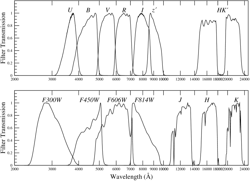
Figure 1: Filter profiles multiplied by the quantum efficiency of the detectors used from our survey (top) and the HDF-N proper (Fernández-Soto et al., 1999) (bottom). All profiles were normalized to have a peak transmission of one.

For data collected with Suprime-Cam a five point X-shaped dither pattern was used with one arc minute steps. The camera was rotated by 90 degrees between dither patterns to remove bleeding from bright stars and provide better photometric calibration. The KPNO-4m data were collected using a nine point grid as a dither pattern with one arc minute steps between pointings. For both the Suprime-Cam and KPNO-4m observations the telescope was offset by 10^′′ in a random direction between dither patterns. The $HK^{\prime}$ data were collected using a 13 point diamond shaped dither pattern with 10^′′ steps between exposures. The filter profiles multiplied by the detector response are plotted in Figure 1 along with the HDF-N filters used in Fernández-Soto et al. (1999). Quantifiable measures of image quality are given in Section 2.4.

2.1 Flat Fielding

All of these data were reduced using Nick Kaiser’s Imcat tools. The $U$, $B$, $V$, $R$, $I$, and $z^{\prime}$ data were first overscan corrected and bias subtracted. Median sky flats were then used to provide a first pass flat fielding. Objects were then masked out and a second flat field was generated for each dither pattern. The second pass flat fielding was necessary to correct for changes in the instruments due to mechanical flexure and rotation of the camera and optics. The sky was then subtracted using a second order polynomial surface fit to the sky for each chip of each image. After the first pass sky subtraction the Suprime-Cam images had time variable scattered light structure left in the images. This problem occurred at the edges of the field where the camera was vignetted and was worst when the moon was up. To correct for this structure the objects were masked out and a surface was tessellated to the sky background and subtracted off.

The $z^{\prime}$ band data taken before April of 2001 were corrected for fringing. To achieve this a surface was tessellated on a 32-pixel grid over the first pass flat field. This surface was used to provide first pass flat fielding instead of the median flat. A median fringe frame was then generated for each night of data, scaled to the background in each image, and subtracted from the flat-fielded images. The images were then second pass flattened and sky subtracted as with the other bands. After April of 2001 new chips were installed that had minimal fringing so fringe subtraction was not performed.

The $U$ band data were corrected for internal pupil reflections which occur on the MOSAIC camera on the KPNO-4m telescope. A pupil image was constructed by dividing the $U$ band flat by a $V$ band flat and masking out the areas that did not contain a pupil reflection. The pupil image was subtracted from the $U$ band flat before flat fielding. The pupil image was then scaled to the background in each image and subtracted off. A second pass flat fielding was then performed for each dither pattern as done for the other bands.

The $HK^{\prime}$ data were collected in 13 point dither patterns so the data could be flattened and sky subtracted separately for each dither pattern using median sky flats. This allowed us to remove the time variability in the bias, flat field, and sky which occurs in IR arrays. The images in each dither pattern were then combined using a weighted mean to provide an image deep enough to map onto the optical astrometry grid. Cosmic rays were removed during the combination process by looking for pixels which lay more than 5$\sigma$ from the weighted mean value. Sigma was calculated from the background noise in each image. Since the image depth varied across the combined, dithered images, an inverse variance map was created for each dither sequence. These inverse variance maps were later used to combine the separate dither sequences.

2.2 Astrometry

An initial solution for the optical distortion was calculated by comparing standard star frames to the USNO-A2.0 (Monet et al., 1998). From this point onward we treated each chip in each exposure as a separate image with a separate distortion. This took into account changes in the optical distortion with time, as well as any mechanical motion on the focal plane.

Using the initial solution we registered images to one another to cross identify point sources from image to image. We also identified any USNO-A2.0 (Monet et al., 1998) stars which were not saturated in our images. Since most USNO-A2.0 objects were saturated in the Suprime-Cam images, the MOSAIC $U$ band data were used for the astrometric solution. The $U$ band data was also chosen because it covers a larger area than the other bands.

At magnitudes fainter than 18 the USNO-A2.0 stars are not properly corrected for magnitude dependent systematics. As well errors for individual stars are not quoted in the USNO-A2.0 and are significantly worse than the mean at the faintest level. As such all USNO-A2.0 stars were assumed to have a Root Mean Square (RMS) uncertainty of 2^′′ in relative astrometry which is larger than any expected systematics.

In the center of the field USNO-A2.0 stars were only used to constrain the scale factor and absolute astrometry of the fit. The relative astrometry was calculated by minimizing the positional scatter of stars which appeared in multiple images. This was done by fitting a third order two-dimensional polynomial to each image. The coefficients of the polynomials were calculated by minimizing the chi-squared defined by equation 1 with respect to the coefficients defined in $f(x,y)$, the polynomial function. In equation 1 $N_{i}$ is the number of images, and $N_{s}$ is the number of stars used for the astrometry. In this equation the USNO-A2.0 is treated as an image, however $f(x,y)$ is replaced with the known star positions. This effectively constrains the scale factor and rotation of the image. Stars which were incorrectly cross-identified between images were removed in an iterative fashion until the astrometric solutions converged.

$$\chi^{2}=\sum_{i=0}^{N_{i}}\sum_{j\neq i}^{N_{i}}\sum_{s=0}^{N_{s}}\frac{[f_{i}(x_{s},y_{s})-f_{j}(x_{s},y_{s})]^{2}}{\sigma_{i}^{2}+\sigma_{j}^{2}}$$ (1)

The resulting relative astrometry should be good to the centroiding error of $\approx 0.1$ pixel or $\approx 0.03$^′′ RMS across the center of the field where there are many measurements for each source. However this method breaks down at the edge of the field where there are fewer images. At the very edge of the field the astrometry is only good to 0.5^′′ since only the USNO-A2.0 constrains the fit hence systematics can not be removed.

Any chromatic aberrations in the astrometry should be minimal since both the KPNO-4m and Suprime-Cam have an atmospheric dispersion corrector. A large number of objects, with a wide range of colors were used for the astrometry, so any residual effects should be averaged out. A more extensive discussion of this issue can be found in Kaiser (2000).

Once an astrometric grid of objects was established, the $B$, $V$, and, $R$ data were warped onto it using a two-dimensional, third order polynomials for each image (still treating each chip separately). To improve the grid in the redder bands point sources from the astrometricaly calibrated $R$ band image were added to the $U$ band astrometric grid. The $I$, $z^{\prime}$, and $HK^{\prime}$ data were warped onto this improved grid in the same way as the bluer data. To provide accurate absolute astrometry the final images were registered to the radio catalog of Richards (2000).

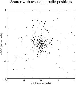
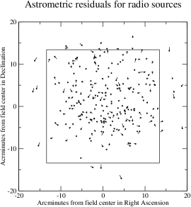
Figure 2: Astrometric residuals with respect to the radio catalog of Richards (2000). The inner box on the left hand side marks the central 0.2 square degrees in the residual map. The vectors point in the direction of the residual and have and amplitude of 60 times the residual in arc seconds.

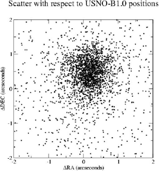
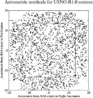
Figure 3: Astrometric residuals with respect to the USNO-B1.0 (Monet et al., 2003). The inner box on the left hand side marks the central 0.2 square degrees in the residual map. The vectors point in the direction of the residual and have and amplitude of 60 times the residual in arc seconds.

We have included comparisons to the radio catalog and USNO-B1.0 (Monet et al., 2003) in Figures 2, and 3. The USNO-B1.0 positions are systematically offset from the radio positions by 0.5^′′ north and 0.2^′′ east (see Figure 3), but this offset was removed before making other comparisons. The RMS astrometric scatter between the our positions and the radio positions over the central 0.2 square degree field is 0.22^′′ . It is 0.32^′′ between our positions and the USNO-B1.0. In both cases the scatter is dominated by the astrometric errors in the reference catalogs which are 0.16^′′ in the radio catalog and 0.34^′′ in the USNO-B1.0 and shows no systematics across the central 0.2 square degree field. As expected we observe systematics with respect to the USNO-B1.0 catalog at the edges of the field, however these offsets are less than 0.5^′′ in amplitude. Furthermore systematics at this level are known to exist in the USNO-B1.0 (Monet et al., 2003) so we chose not to remove them.

2.3 Image Warping And Combination

For the $U$, $B$, $V$, $R$, $I$, and $z^{\prime}$ data chip-to-chip photometric scaling factors were calculated for each dither pattern. This was necessary because each dither pattern was flattened separately which can change the relative normalization of the chips. When collecting our data we used large steps in our dither patterns and rotated the camera when possible. This meant we could always find a reference chip which covered the same area of sky as two or more chips in another exposure. The scaling between two chips in one exposure could then be calculated by comparing their scaling factors to a chip in another exposure. This was independent of exposure to exposure scaling so long as the photometry did not vary across the reference chip. To calculate the scale factors we used 6^′′ apertures on objects detected at greater than 50$\sigma$ with half light radii less than 1.5^′′ . The large apertures were used to prevent any variations in seeing from affecting the scaling. The large number of exposures meant we made many measurements of the chip-to-chip scaling between adjacent chips. These were combined in a weighted mean. Once the chip-to-chip photometric scaling was removed, exposure to exposure scale factors were calculated in a similar fashion by comparing overlapping areas between exposures.

The geometric distortions in the MOSAIC and Suprime Cam optics cause each pixel to have a different effective area on the sky. By flat fielding these images we introduce a geometry dependent photometric offset. When calculating the photometric scaling we corrected for this effect.

The $HK^{\prime}$ data consists of 210 dither patterns of 13 images each. These data were collected under a combination of photometric and non-photometric conditions. We collected these data in such a way that each dither overlapped several neighboring dither patterns. To correct the photometry we calculated scale factors for each dither pattern such that the photometric scatter was minimized across the field in the overlapping regions. The absolute zero point was allowed to float during this procedure and later tied to the Fernández-Soto et al. (1999) catalog (see §2.5).

Saturated pixels were clipped in the $U$ band images before warping or combination. However saturated pixels in the Suprime-Cam behaved in a very non-linear fashion, often dropping or ringing in value as they became more saturated. As such we could not simply clip the saturated pixels. We removed the saturation spikes along with satellite trails by searching for strings of elongated objects which formed straight lines in the images. A strip 21 pixels wide was clipped from the images along detected lines.

After applying photometric corrections each image was warped onto a stereographic projection. We corrected the geometry dependent photometric scaling by choosing a mapping which preserved surface brightness. The re-sampling was done using a nearest neighbor algorithm. A weighted mean was then calculated for each pixel, pixels which lay more than 5$\sigma$ from the mean were rejected to remove cosmic rays. For the $U$, $B$, $V$, $R$, $I$, and $z^{\prime}$ data the sigma used in the rejection and weighting was measured from the RMS background noise in the un-warped image. For the $HK^{\prime}$ images a sigma was calculated for each pixel during the dither pattern combination and carried through to the final image combination. To avoid clipping pixels which varied due to seeing variations a window was defined around the median of the pixel values. If a pixel value were between half to twice the median value of all pixels it was accepted even if it were more than 5 sigma from the mean. A weighted mean and inverse variance were then calculated for all accepted pixels.

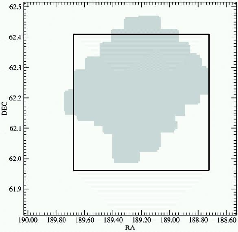
Figure 9: The area with $HK^{\prime}$ coverage is shaded in grey, the catalog area is shown by the black outline, please note that the $HK^{\prime}$ data does not cover the whole catalog area.

The quality of the final images is displayed in Figures 4a-4d where we compare cutouts of our data in the HDF-N proper region with the Hubble Space Telescope images of Williams et al. (1996) The area with $HK^{\prime}$ data is shown in Figure 9.

2.4 Object Detection and Measurement

The catalog of objects was detected in the $R$ and $z^{\prime}$ band images using Sextractor (Bertin & Arnouts, 1996). Objects with three or more pixels rising more than 1.5$\sigma$ above the background were analyzed, but only those with 5$\sigma$ measurements of their aperture flux were output to the catalog. The significance of a detection was calculated using the RMS map generated during the image combination process. The absolute scaling of the RMS map was calculated by laying down random blank apertures away from objects on the images. This was done since the pixel-pixel noise underestimates the image noise. This method may somewhat overestimate the true noise since it also includes variations due to faint objects in the blank apertures. The area around bright stars was masked out to prevent erroneous detections and measurements from scattered light.

We calculated both aperture and isophotal magnitudes for our images. Aperture magnitudes were selected as the primary magnitude to avoid biases introduced by galaxy morphology in isophotal magnitudes. To avoid filter dependent aperture corrections the images were smoothed with a Gaussian to match the median ratio of the total to the aperture magnitude in the worst seeing ($U$ band) image. We chose this method because it ensures the apertures are sampling the same percentage of the total light in all bands and does not assume the PSF is gaussian. PSF matching provided a lower signal to noise because it includes the non-gaussian components of all seven PSF’s which degraded the image quality. The aperture magnitudes were calculated on these smoothed images while the isophotal magnitudes were calculated on the un-smoothed images. A 3^′′ diameter aperture was used for the photometry. An annulus with an inner radius of 6^′′ and outer radius of 12^′′ was used for sky subtraction. The 5 sigma limiting magnitude cut was calculated using aperture magnitudes on the un-smoothed image to avoid losing faint objects.

For the $V$ band data we included archival data to increase the depth (Iwata et al., 2003). These data had better seeing (0.71^′′ compared to 1.18^′′ ); however they did not cover our entire field. Furthermore these data were taken with extremely long exposures which become non-linear at $\simeq$22nd magnitude To avoid position dependent image quality and saturation, we reduced the archival data separately and scaled them to have matching photometry. Where archival data existed and was unsaturated, it was used for the shape measurements. Photometry was performed on the two images separately and the fluxes combined using a weighted mean.

2.5 Absolute Photometry

The HDF-N is a heavily observed area of the sky with extremely accurate photometry in many bands. Many objects have known redshifts and spectral energy distributions making it easy to check the accuracy of our photometry. Furthermore it is difficult to accurately measure standard stars with Suprime-Cam because of the size of the telescope and overheads involved. Obtaining photometry on other telescopes would introduce problems similar to those in using the existing photometry. As such we have chosen not to use standard stars, but rather calibrate the data using the existing photometry.

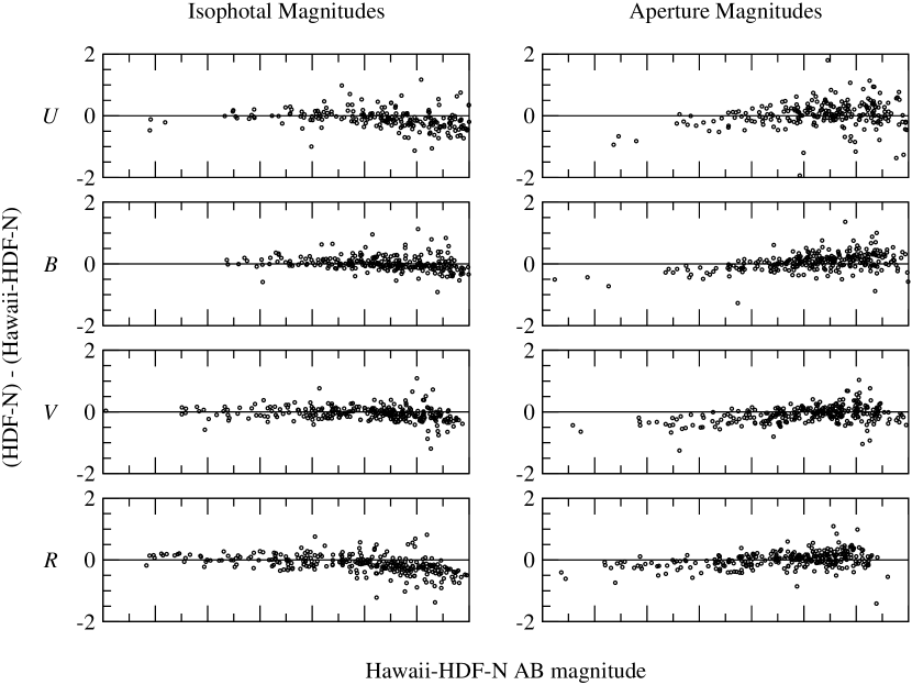
Figure 10: Comparison of our photometry to that of Fernández-Soto et al. (1999) from the HDF-N. The magnitudes have been converted to our filter system by linearly interpolating the flux between the HDF-N filters. The RMS scatter between our isophotal magnitudes and those of Fernández-Soto et al. is 0.19 magnitudes on average which corresponds to an average error of 0.03 magnitudes in the zero points.

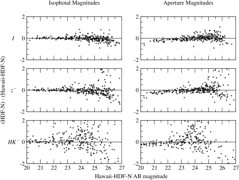
Figure 11: Comparison of our photometry to that of Fernández-Soto et al. (1999) from the HDF-N. The magnitudes have been converted to our filter system by linearly interpolating the flux between the HDF-N filters. The RMS scatter between our isophotal magnitudes and those of Fernández-Soto et al. is 0.19 magnitudes on average which corresponds to an average error of 0.03 magnitudes in the zero points.

To obtain accurate absolute photometry in the AB system we matched our photometry to the HDF-N photometry of Fernández-Soto et al. (1999) who carefully corrected for many subtle photometric effects in the HDF-N data. We converted the fluxes in the Fernández-Soto et al. catalog to our filter system by linearly interpolating the flux between the HDF-N filters. The effective wavelength of the filters were used for the interpolation. This method weights by transmission so any overlap between the Fernández-Soto et al. (1999) filters and ours should be accounted for. We then compared our isophotal fluxes to the ones we interpolated and scaled them to match. Since the Fernández-Soto et. al. fluxes were measured in an isophotal aperture, they vary systematically in magnitude with respect to the flux measured in a fixed aperture. To prevent this from introducing filter dependent offsets in our aperture fluxes we used the same magnitude range of 22-24 $AB_{mag}$ in the $U$, $B$, $V$, $R$, $I$, and $z^{\prime}$ bands when comparing our aperture photometry to the Fernández-Soto et. al. photometry. In the $HK^{\prime}$ band we were forced to use a range of 22-23.5 because of the shallower data. This may have introduced a small bias in our photometry for this band. We then scaled the aperture magnitudes to total magnitudes by comparing our isophotal and aperture fluxes for point sources in the $I$ band. $I$ band was chosen because it had the best image quality of the red bands and closely approximated the $F814W$ filter used in the HDF-N. To quantify the error in our zero point determination we measured the RMS scatter between our isophotal magnitudes and those of Fernández-Soto et. al. The RMS scatter is 0.19 magnitudes which corresponds to and average error of 0.03 magnitudes in our photometric zero points exact numbers for all bands are given in table 3. Figures 10 and 11 compares our final photometry to the interpolated photometry of Fernández-Soto et al. (1999).

Since an extensive catalog of spectroscopic redshifts (Cohen et al., 2000) exists for this field it is possible to compare our photometry to galaxy templates. This comparison was done using the photometric redshift code of Benítez (2000) which includes a calibration mode. First a best fit template at the known redshift was found for each object. The templates of Coleman et al. (1980) and Kinney et al. (1996) were used. Twenty intermediate spectra were interpolated between the main spectral templates to improve the fits. Then a weighed mean offset was calculated for each filter by comparing our photometry to the template photometry. These offsets were then applied to our photometry and the process repeated until the offsets converged. We did not apply offsets the $B$ and $I$ magnitudes because they are close to the HDF-N $F450W$ and $F814W$ filters respectively and hence we expect them to be correctly calibrated. The resulting offsets are small and are probably due to inaccuracies in the templates or filter profiles (see Table 3). The largest offsets occur in the $R$, $z^{\prime}$, and $HK^{\prime}$ bands which are also those least like the HDF-N filters. The large offset in $HK^{\prime}$ may also be due to the different magnitude range used when scaling the aperture fluxes.

2.6 Catalog Description

Due to the large amount of data we have broken the catalog into several files which are available on the Internet. There are two catalogs, one selected in the $R$ band and the other in the $z^{\prime}$ band. Objects with an aperture magnitude error smaller than 5 sigma on the un-smoothed images in the selecting band were included. If an object was present in both catalogs it was removed from the $z^{\prime}$ catalog. Each object has a unique ID within each catalog, but both the $R$ and $z^{\prime}$ catalog begin at 1. Our data covers up to 0.4 square degrees in some bands, however around the edges the coverage is un-even, the astrometry may be distorted (see §2.2), and the detections become unreliable due to cosmic rays, reflections and other defects which could not be removed. As such we avoided these regions for our scientific objectives. All results in this paper are from the central 0.2 square degrees where the data is of equal depth in the $U$, $B$, $V$, $R$, $I$, and $z^{\prime}$ bands. Since others may find it useful we have included data for the entire field in supplementary files with the same formatting and content as the main catalog. However we strongly recommend using only the main $R$ and $z^{\prime}$ catalog containing objects in the central 0.2 square degrees. No attempt was made to ensure the integrity of the data outside the central area.

Each catalog consists of four files, the contents of which are listed in tables 4,5,6,7. The shape file contains information on the position and morphology of the object output by Sextractor. The flag file contains flags for saturation, overlapping objects, and questionable or bad detections. The bad flag is set for objects with a Full Width at Half Max (FWHM) of 0 or with abnormal magnitudes in the selection band. This flag was intended to mark questionable detections, however some faint point sources may also have been flagged. The magnitude file contains aperture and isophotal magnitudes along with errors in the AB system for all bands. We used the Sextractor convention of -99 for an object which was outside the field or which could not be measured for other reasons. Badly saturated objects were also given a magnitude of -99. Objects with negative fluxes were assigned negative magnitudes with the absolute value of the magnitudes corresponding to the absolute value of the flux. The flux catalog contains aperture and isophotal fluxes along with errors and background levels. All measurements in the flux file are in nano-Janskys (nJy).

The area around bright objects has been removed due to false detections and problematic photometry in these areas. This was done by cutting out circles around USNO-A2.0 objects with magnitudes brighter than 15.5. A list of these regions and the size of each cutout is provided along with the catalog.

3 Results

3.1 Number Counts

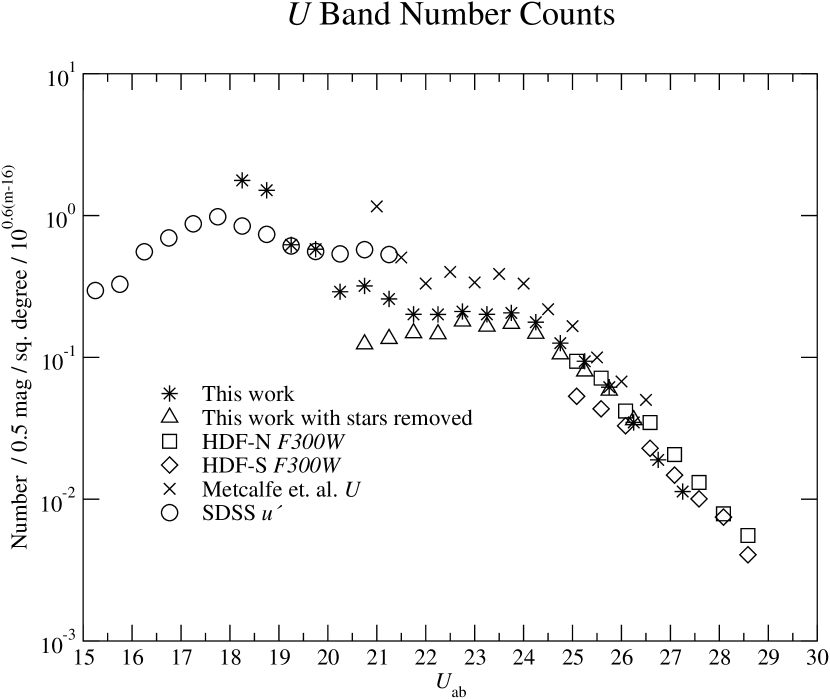
Figure 12: U band number counts from this work, the Herschel Deep Field (Metcalfe et al., 2001), the HDF-N (Metcalfe et al., 2001), and the Sloan Digital Sky Survey (SDSS) (Yasuda et al., 2001). Objects were identified as stars if they had a value of 0.9 or greater in the Sextractor star galaxy-separator.

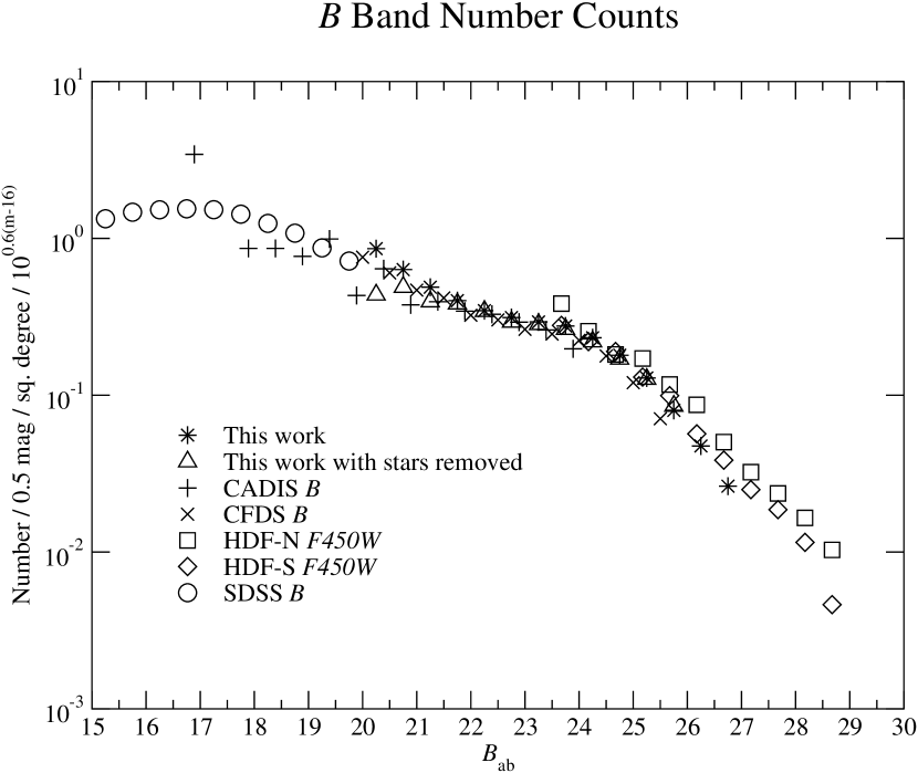
Figure 13: B band number counts from this work, the Calar Alto Deep Imaging Survey (Huang et al., 2001), the Canada France Deep Survey (CFDS)(McCracken et al., 2001), the HDF-N (Metcalfe et al., 2001), and the Sloan Digital Sky Survey (SDSS) (Yasuda et al., 2001). Objects were identified as stars if they had a value of 0.9 or greater in the Sextractor star galaxy-separator.

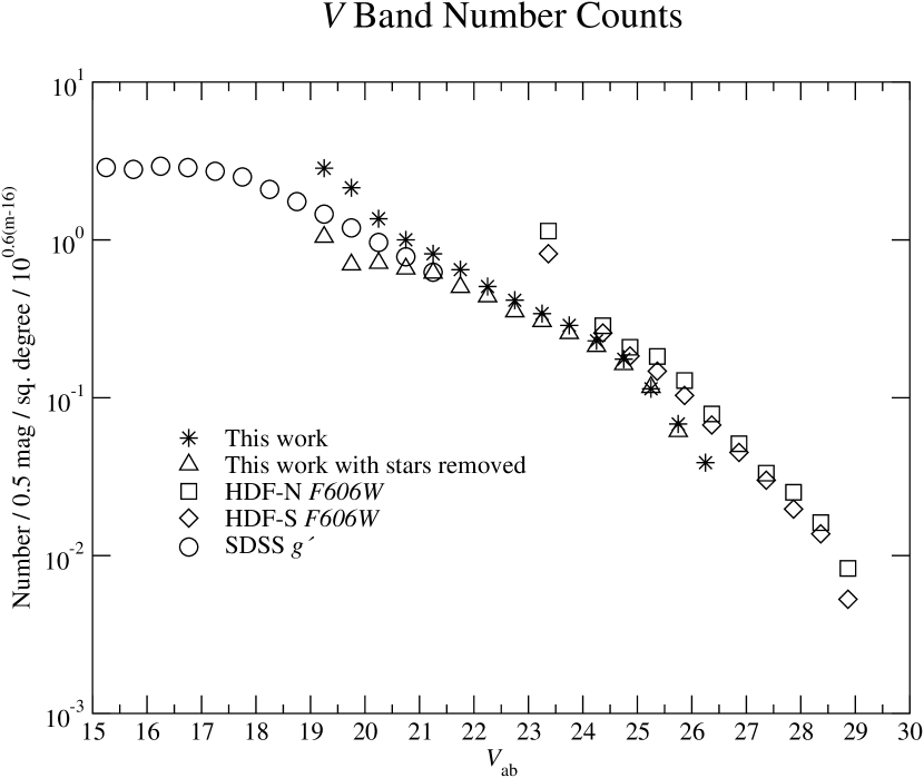
Figure 14: V band number counts from this work, the HDF-N (Metcalfe et al., 2001), and the Sloan Digital Sky Survey (SDSS) (Yasuda et al., 2001).

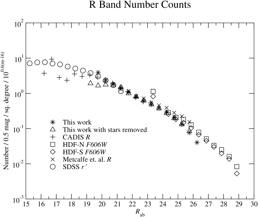
Figure 15: R band number counts from this work, the Calar Alto Deep Imaging Survey (Huang et al., 2001), the Herschel Deep Field (Metcalfe et al., 2001), the HDF-N (Metcalfe et al., 2001), and the Sloan Digital Sky Survey (SDSS) (Yasuda et al., 2001). Objects were identified as stars if they had a value of 0.9 or greater in the Sextractor star galaxy-separator.

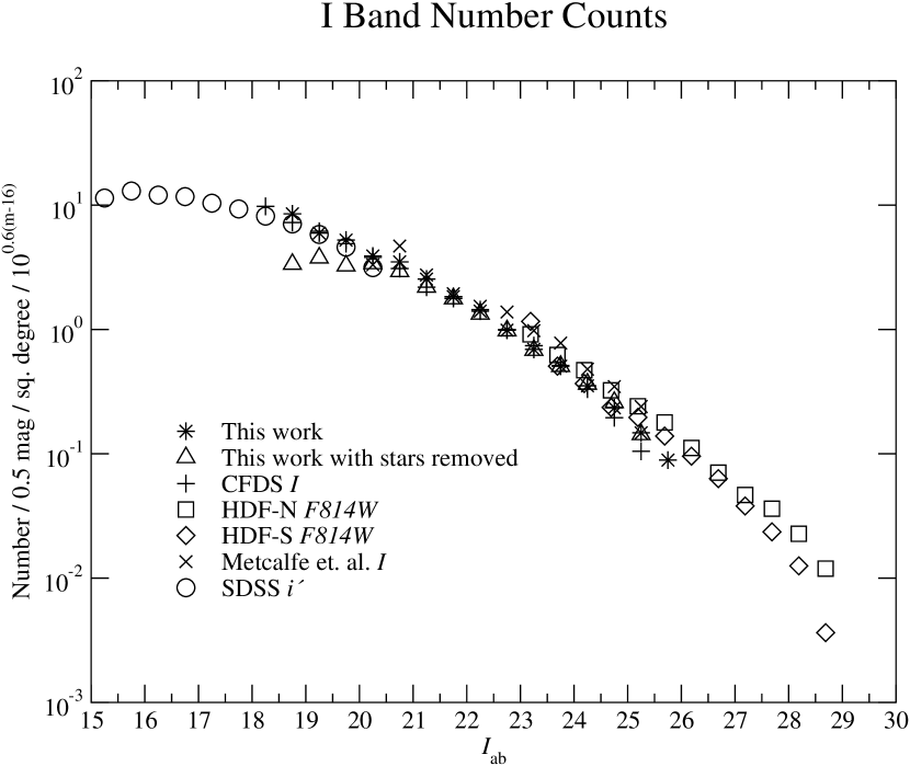
Figure 16: I band number counts from this work, the Canada France Deep Survey (CFDS)(McCracken et al., 2001), the Herschel Deep Field (Metcalfe et al., 2001), the HDF-N (Metcalfe et al., 2001), and the Sloan Digital Sky Survey (SDSS) (Yasuda et al., 2001). Objects were identified as stars if they had a value of 0.9 or greater in the Sextractor star galaxy-separator.

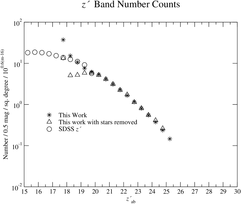
Figure 17: $z^{\prime}$ band number counts from this work and the Sloan Digital Sky Survey (SDSS) (Yasuda et al., 2001). Objects were identified as stars if they had a value of 0.9 or greater in the Sextractor star galaxy-separator.

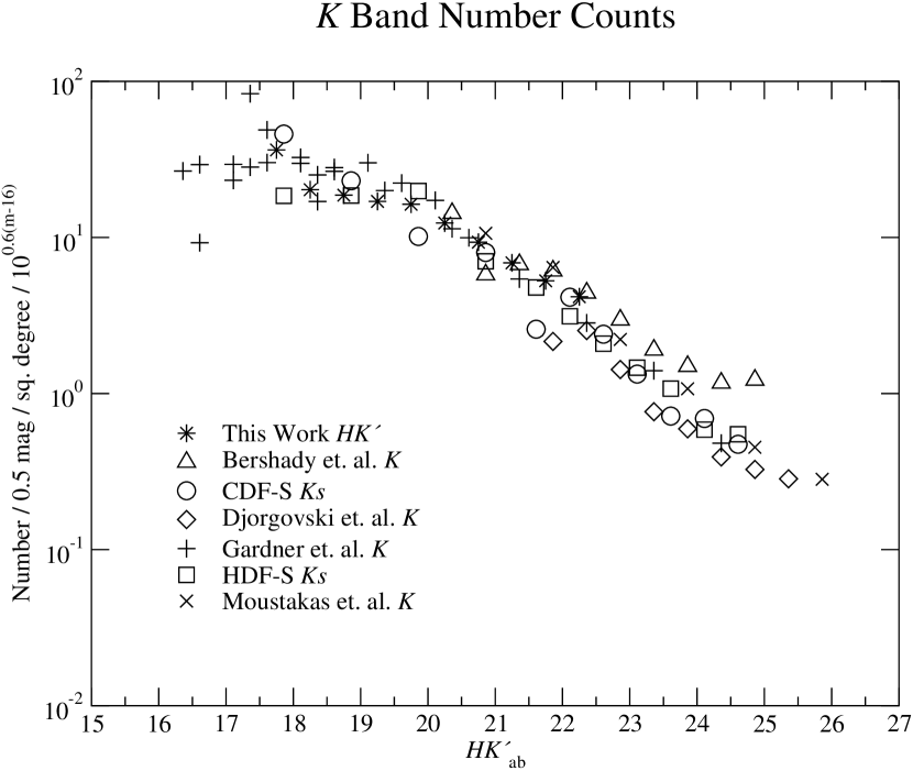
Figure 18: K band number counts from this work, the Chandra Deep Field South (CDF-S) (Saracco et al., 2001), the HDF-N (Saracco et al., 2001), and several other authors (Bershady et al., 1998; Moustakas et al., 1997; Djorgovski et al., 1995; Soifer et al., 1994; Gardner et al., 1993) are over plotted. An offset of 1.859 was applied to Vega magnitudes to convert them to the AB system.

To determine number counts we constructed separate catalogs detected in each color using the un-smoothed images. We measured fluxes in 3^′′ diameter apertures and applied an aperture correction to each band. We did not use the Sextractor best or isophotal magnitudes because they often act in a non-linear way at low signal to noise. The correction was calculated by measuring the median offset between Sextractor best magnitudes (Bertin & Arnouts, 1996), which estimate total magnitudes, and the aperture magnitudes for objects brighter than 24th magnitude (see Table 3). Using aperture magnitudes may introduce a magnitude dependent bias in the number counts. However we saw no evidence that the median correction was changing with magnitude. Due to the difficulty in identifying stars at faint magnitudes we have provided both raw counts and counts with stars removed. Objects were identified as stars if they had a value of 0.9 or greater in the Sextractor star galaxy-separator. We did not remove stars in the $HK^{\prime}$ band because the star galaxy separator was unreliable in that band due to variable seeing across the image. The number counts shown in Figures 12-18 were normalized to a Euclidean slope as described in Yasuda et al. (2001). They agree with those reported by other authors (Metcalfe et al., 2001; McCracken et al., 2001; Huang et al., 2001; Yasuda et al., 2001; Saracco et al., 2001; Djorgovski et al., 1995; Soifer et al., 1994; Gardner et al., 1993). The Sloan Digital Sky Survey counts (Yasuda et al., 2001) were measured in $u^{\prime}$, $g^{\prime}$, $r^{\prime}$, $i^{\prime}$, and $z^{\prime}$ which are close to our bands with the exception of $g^{\prime}$ and $r^{\prime}$. The Sloan $B$ band counts were generated by extrapolating between the $u^{\prime}$, $g^{\prime}$, and $r^{\prime}$ bands (Yasuda et al., 2001). To facilitate comparisons by future authors we have fit an exponential of the form $N=B10^{A(magnitude)}$ to our bright end counts where N is in number per square degree per magnitude. The results of these fits are quoted in table 8. The number count data are also provided in tables 9 and 10.

3.2 Selection of High Redshift Objects

High redshift galaxies have unique colors due to the Lyman break at 912Å  and Lyman alpha absorption blueward of 1216Å. We can select theses galaxies by choosing three filters which fall blueward of the Lyman break, between the Lyman break and Lyman alpha line, and redward of Lyman alpha respectively. Steidel et al. (1999, 1995) successfully uses a set of customized filters to select galaxies at $z\simeq 3$ and $z\simeq 4$. Their spectroscopic followup is over 80% success in identifying $z\simeq 3$ galaxies. Metcalfe et al. (2001) has also used these criteria on the Herschel Deep Field and HDF-N.

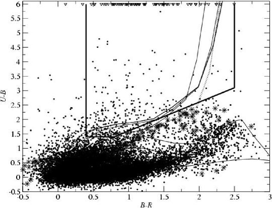
Figure 20: $(B-R)$ vs. $(U-B)$ color-color plot for all objects with $B_{AB}>26$. The region indicated by heavy lines in the top right is where we expect to find $z\simeq 3$ objects similar to those of Steidel et al. (1995). The light solid lines show the expected evolution of Coleman et al. (1980) galaxy templates and the dotted lines the Kinney et al. (1996) SB2 and SB3 galaxy templates. The expected colors of stars from Pickles (1998) are over plotted as stars. The downward facing triangles at $(U-B)=6$ are objects which were not detected in U.

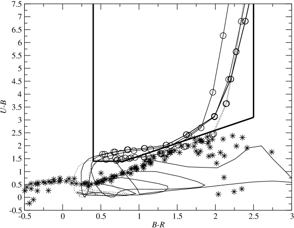
Figure 21: $(B-R)$ vs. $(U-B)$ color-color plot with galaxy tracks. The region indicated by heavy lines in the top right is where we expect to find $z\simeq 3$ objects similar to those of Steidel et al. (1995). The light solid lines show the expected evolution of Coleman et al. (1980) galaxy templates and the dotted lines show the Kinney et al. (1996) SB2 and SB3 galaxy templates. The expected colors of stars from Pickles (1998) are over plotted as stars. Circles indicate galaxies in the $2.5<z<3.5$ redshift range selected by Steidel et al. (1995).

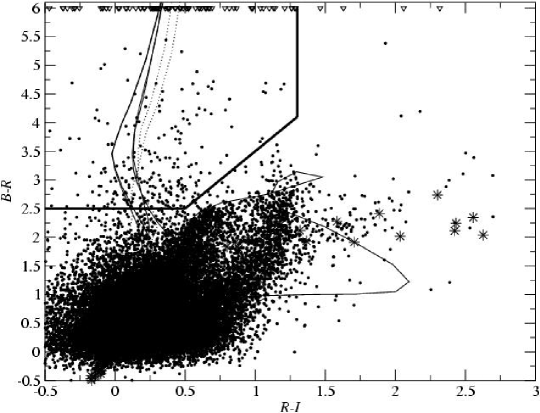
Figure 22: $(R-I)$ vs. $(B-R)$ color-color plot for all objects with $R_{AB}>26$. The region indicated by heavy lines in the top left is where we expect to find $z\simeq 4$ objects similar to those of Steidel et al. (1999). The light solid lines show the expected evolution of Coleman et al. (1980) galaxy templates and the dotted lines show the Kinney et al. (1996) SB2 and SB3 galaxy templates. The expected colors of stars from Pickles (1998) are over plotted as stars. The downward facing triangles at $(B-R)=6$ are objects which were not detected in B.

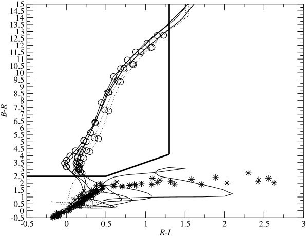
Figure 23: $(R-I)$ vs. $(B-R)$ color-color plot with galaxy tracks. The region indicated by heavy lines in the top left is where we expect to find $z\simeq 4$ objects similar to those of Steidel et al. (1999). The light solid lines show the expected evolution of Coleman et al. (1980) galaxy templates and the dotted lines show the Kinney et al. (1996) SB2 and SB3 galaxy templates. The expected colors of stars from Pickles (1998) are over plotted as stars. Circles indicate galaxies in the $3.5<z<4.8$ redshift range selected by Steidel et al. (1995).

The number and type of object selected are strongly dependent on the filters and selection criteria used. Changing these parameters can severely effect the success in identifying high redshift galaxies and change the redshift range selected. For comparison to the previous work we need to select the same population as Steidel et al. (1999, 1995) and Metcalfe et al. (2001). However our band passes differ significantly from theirs. We corrected this by calculating the expected colors for the galaxies they have selected. These colors are calculated by integrating the galaxy templates of Coleman et al. (1980) and Kinney et al. (1996) moderated by our filter response profile. We correct these templates for Ly_α and Ly_β absorption following the prescription of Madau (1995). We also calculate the expected colors of stars using the spectral library of Pickles (1998). We then set a selection criteria which will select similar galaxies to the previous work but avoids stars. The resulting selection is shown in Figures 21 and 23 along with color-color tracks for various galaxy types. The selection is also shown along with our data in figures 20 and 22.

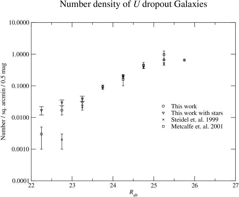
Figure 26: The raw sky density of $U$ band dropouts uncorrected for contamination or incompleteness are shown. Error bars are 1$\sigma$ poison fluctuations for Metcalfe et al. (2001) and our data. The errors for Steidel et al. (1999) include an estimate of cosmic variance from their multiple fields. Much of the variation between the counts is likely due to cosmic variance.

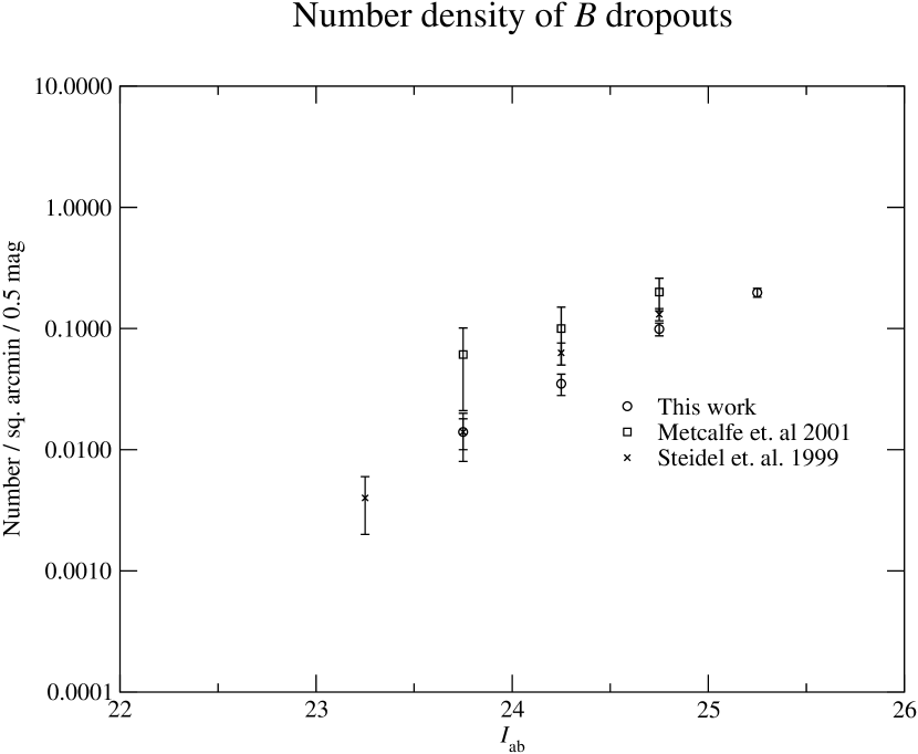
Figure 27: The raw sky density of $B$ band dropouts uncorrected for contamination or incompleteness are shown. Error bars are 1$\sigma$ poison fluctuations for Metcalfe et al. (2001) and our data. The errors for Steidel et al. (1999) include an estimate of cosmic variance from their multiple fields. Much of the variation between the counts is likely due to cosmic variance.

The surface density we measure using this selection is similar to that measured by other authors (Metcalfe et al., 2001; Steidel et al., 1999) (see Figures 26,27 and tables 11,12. Due to our redder $U$ band filter the $z\simeq 3$ selection suffers more contamination from stars and low redshift galaxies than that of Steidel et al. (1999, 1995). We attempted to remove stars by selecting objects with $R<23.5$ and $R_{fwhm}>1.3\arcsec$ as describe in McCracken et al. (2001), however the contamination from galaxies remains. At magnitudes fainter than $R=23$ our measurements are within the one sigma error bars reported by Steidel et al. (1999, 1995) and Metcalfe et al. (2001). Our B band counts are consistent with but systematically lower than those of Steidel et al. (1999) or Metcalfe et al. (2001) which is likely due to cosmic variance.

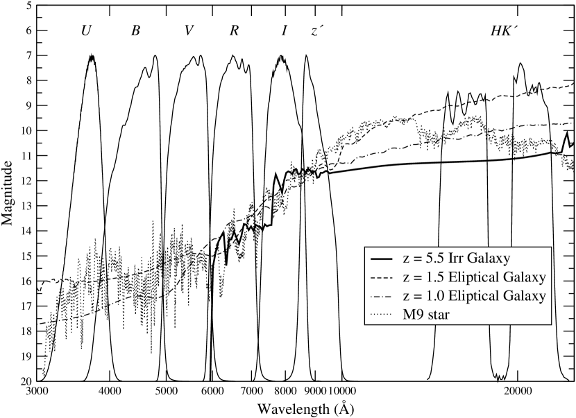
Figure 19: The expected Spectral Energy Distribution (SED) of a $z=$ 5.5 star forming, $z=$ 1.5 Elliptical, and $z=$ 1.0 Elliptical galaxy from the Coleman et al. (1980) library are shown along with an M9 star from Pickles (1998). These SED’s were corrected for intergalactic absorption using Madau (1995). The filter profiles of our survey are overlaid for comparison. Note the similarity of the SED’s in $R$, $I$, and $z^{\prime}$ bands. Note that differentiating the $z=5.5$ Irr from the $z=1.0$ or $z=1.5$ elliptical requires multi-color information and is most sensitive in the $U$, $B$, and near-IR bands. The maximum information comes from the largest wavelength range sample.

The selection at redshifts higher than $z\simeq 4$ is significantly more difficult. The contamination for $z\simeq 3$ galaxies comes from low redshift galaxies where the co-moving volume is small. For $z>5$ galaxies the contamination comes from $z\simeq 1$ where the effective co-moving volume is very large. Several authors have recently reported the discovery of large numbers of $z>5$ galaxies using color-color selection (Iwata et al., 2003; Lehnert & Bremer, 2003). However we find their two color selection yields a large number of lower redshift galaxies. Figure 19 shows an example for a redshift 5.5 galaxy. Elliptical galaxies at $1<z<1.5$ have similar colors to a $z>5.5$ galaxy in the $R$, $I$, and $z^{\prime}$ bands. The only clear difference is in the bluer or redder bands. In particular the use of an $(R-I)$ selection will include many low redshift galaxies. A similar problem will occur at redshift 6 using an $(I-Z)$ selection. There is no easy solution, either one must go more than three magnitudes deeper in the bluest band than the reddest, or obtain deep near IR imaging, both of which are time intensive for large surveys.

Songaila et al. (1990) sets out a clear criteria for selecting high redshift galaxies based on the Lyman alpha absorption shown in equation 2.

$$\Delta m_{Lycont}=3.8+20.3log_{10}\left(\frac{1+z}{7}\right)$$ (2)

For $z>5$ galaxies it requires $(V-I)>2.4$ and no detection blueward of the 912Å break. Using these criteria and our multi-color data we can test the findings of other authors. To test the level of contamination we have restricted ourselves to $z^{\prime}>25$ which is bright enough for the expected contaminating sources to be detected at 2$\sigma$ in $U$ or $B$ bands.

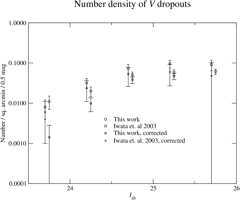
Figure 28: The raw sky density of $V$ band dropouts and an estimate of the density corrected for contamination are shown for the Hawaii-HDF-N. Neither measurement is corrected for incompleteness. Error bars are 1$\sigma$ poison fluctuations. The counts of Iwata et al. (2003) are higher due to a higher rate of contamination.

Iwata et al. (2003) imaged the same area with Suprime-Cam in the same $V$, $I$, and $z^{\prime}$ filter we used. However they calibrated their data in a different manner. We adopted $(V-I)\geq 2.4$ and $(V-I)\geq 7(I-z^{\prime})-0.2$ as our selection criteria. This avoids selecting $z\simeq 1$ galaxies and late type stars. We find that our counts are consistent with, but lower than the values of Iwata et al. (2003) (see Figure 28 and Tables 13 and 14). Moving our selection slightly redder in $(I-Z)$ color increases the number of objects selected, making our numbers more consistent with Iwata et al. (2003). However all the additional objects are detected in $U$ or $B$ band. Even when objects detected in $U$ or $B$ are removed, many of the remaining objects in the ACS GOODS field morphologically appear to be stars (this will be quantified elsewhere). These results suggest that a combination of $z\simeq 1$ galaxies and late type stars are contaminating the $z>5.5$ selection.

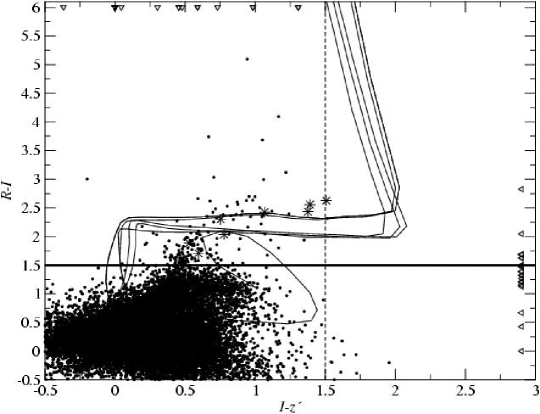
Figure 25: $(I-z^{\prime})$ vs. $(R-I)$ color-color plot for all detected objects. The heavy line at $(R-I)=1.5$ indicates the selection criteria of Lehnert & Bremer (2003) and the dashed line at $(I-Z)=1.5$ is the selection criteria of Stanway et al. (2003). The light solid lines show the expected evolution of Coleman et al. (1980) galaxy templates and the Kinney et al. (1996) SB2 and SB3 galaxy templates. The expected colors of stars from Pickles (1998) are over plotted as stars. The downward pointing triangles at $(R-I)=6$ are objects which were not detected in R and leftward pointing triangles at $(I-Z)=6$ are objects which were not detected in I.

Figure 25 shows that the selection criteria of Lehnert & Bremer (2003) is very likely selecting low redshift galaxies or stars. We find that 95% of the objects selecting using this criteria are detected at 2$\sigma$ in $V$. This selection is particularly problematic since it may include star forming galaxies at $z<2$ where [O III] or [O II] can be mistaken for Lyman $\alpha$. Finally the $(I-Z)>1.5$ selection used by Stanway et al. (2003), selects objects which are detected at 2$\sigma$ in $V$ band 53% of the time. In contrast only 14% of objects selecting using the $(B-R)$, $(R-I)$ selection were detected in $U$ band. Based on our number counts the probability of an object at 28^th magnitude falling into a 3^′′ aperture by chance is 37% in $V$ band and 4% in $U$ band. This implies that color selection may be overestimating the number of high redshift galaxies and hence the star formation rates at $z>5$. We shall give a more extensive discussion of this issue with photometric redshift estimates in a future paper (Capak et al., 2003).

3.3 Conclusion

We have compiled a deep, multi-color catalog over 0.2 square degrees in the HDF-N region. These data will provide an invaluable basis for understanding the formation and evolution of galaxies by providing a large sample of galaxies which can be studied in various ways. The raw number counts and counts of $z\simeq 3$, and $z\simeq 4$ galaxies agree with those of other authors. However the selection of $z>5$ galaxies suffers from significant contamination by low redshift galaxies. The current deep blue imaging is required to reliably selected these galaxies and hence estimate the star formation rate.

Figure 4a: On the left is a cutout image of our data around the HDF-N proper in $U$ band, and on the right is the Hubble space telescope $F300W$ band image for comparison(Williams et al., 1996). Note the depth and quality of the ground based image.

Figure 4b: On the left is a cutout image of our data around the HDF-N proper in $B$ band, and on the right is the Hubble space telescope $F450W$ band image for comparison(Williams et al., 1996). Note the depth and quality of the ground based image.

Figure 4c: On the left is a cutout image of our data around the HDF-N proper in $V$ band, and on the right is the Hubble space telescope $F606W$ band image for comparison(Williams et al., 1996). Note the depth and quality of the ground based image.

Figure 4d: On the left is a cutout image of our data around the HDF-N proper in $I$ band, and on the right is the Hubble space telescope $F814W$ band image for comparison(Williams et al., 1996). Note the depth and quality of the ground based image.

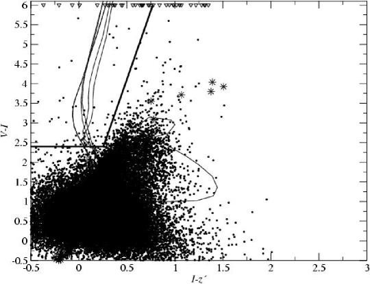
Figure 24: $(I-z^{\prime})$ vs. $(V-I)$ color-color plot for all detected objects. The region indicated by heavy lines in the top left is where we expect to find $z\simeq 5.5$ objects based on the criteria of Iwata et al. (2003). We have moved the cuts to $(V-I)>=2.4$ and $(V-I)>7(I-Z)-0.2$ to avoid contamination from lower redshift galaxies and late type stars as well as account for differences in the photometric system. The expected colors of stars from Pickles (1998) are over plotted as stars. The downward facing triangles at $(V-I)=6$ are objects which were not detected in V.

Table 1: Telescopes used, Exposure Times, and Dates of Observations

Band	Integration	Telescope	Typical	Date of
	Time (h)	Used	Integration (s)	Observations
$U$	28.5	KPNO 4m	1800	2002, March, 9-13
$B$	1.7	Subaru 8.3m	600	2001, February, 27,28
$V$	6.4	Subaru 8.3m	1200	2001, February, 23,24
	2.0		600	2001, March 21-23
$R$	5.2	Subaru 8.3m	480	2001, February, 27,28
			600	2001, March, 21-23
$I$	2.9	Subaru 8.3m	300	2001, February, 23,24
			300	2001, March, 21-23
			300	2002, April, 5,11-14
$z^{\prime}$	3.9	Subaru 8.3m	180	2001, February, 23,24,27,28
			240	2000, March, 21-23
$HK^{\prime}$	0.43	UH 2.2m	120	1999-2002

Table 2: Data Quality, Depth, and Coverage

Band	Seeing	$5\sigma$ limit	Total area	Deep area	Date of
	arcsecond	(AB mag)	Covered (deg2)	Covered (deg2)	Observations
$U$	1.26	27.1	0.40	0.36	2002, March, 9-13
$B$	0.71	26.9	0.27	0.20	2001, February, 27,28
$V$	0.71	26.8	0.27	0.20	2001, February, 23,24
	1.18		0.40	0.20	2001, March 21-23
$R$	1.11	26.6	0.27	0.20	2001, February, 27,28
			0.40	0.20	2001, March, 21-23
$I$	0.72	25.6	0.27	0.20	2001, February, 23,24
			0.40	0.20	2001, March, 21-23
			0.40	0.20	2002, April, 5,11-14
$z^{\prime}$	0.67	25.4	0.27	0.20	2001, February, 23,24,27,28
			0.40	0.20	2000, March, 21-23
$HK^{\prime}$	0.87	22.1	0.11	0.11	1999-2002

Table 3: Photometric Information

Band	Zeropoint	Offsets from	Aperture	Offsets to	Central	Bandpass Å
	Error	SED fitting	Correction	Vega system	Wavelength Å
$U$	0.031	-0.008	-0.311	0.719	3647.65	387.16
$B$	0.028	0.000	-0.159	-0.077	4427.60	622.05
$V$	0.028	-0.005	-0.282	0.023	5471.22	577.36
$R$	0.026	0.061	-0.262	0.228	6534.16	676.39
$I$	0.016	0.000	-0.126	0.453	7975.89	792.89
$z^{\prime}$	0.018	-0.065	-0.147	0.532	9069.21	802.63
$HK^{\prime}$	0.042	-0.181	-0.233	1.595	18947.38	5406.22

Table 4: Contents of Shape File

Column Number	Shape Catalog Item
1	ID
2	RA(J2000)
3	DEC(J2000)
4	x position on image
5	y position on image
6	$U$ FWHM
7	$U$ Semi-Major Axis
8	$U$ Semi-Minor Axis
9	$B$ FWHM
10	$B$ Semi-Major Axis
11	$B$ Semi-Minor Axis
12	$V$ FWHM
13	$V$ Semi-Major Axis
14	$V$ Semi-Minor Axis
15	$R$ FWHM
16	$R$ Semi-Major Axis
17	$R$ Semi-Minor Axis
18	$I$ FWHM
19	$I$ Semi-Major Axis
20	$I$ Semi-Minor Axis
21	$z^{\prime}$ FWHM
22	$z^{\prime}$ Semi-Major Axis
23	$z^{\prime}$ Semi-Minor Axis
24	$HK^{\prime}$ FWHM
25	$HK^{\prime}$ Semi-Major Axis
26	$HK^{\prime}$ Semi-Minor Axis

Table 5: Contents of Flag File

Column Number	Flag Catalog Item	Comments
1	ID
2	Bad	Set to 1 if the FWHM is 0 in the detecting band
3	$U$ Saturated	Set to 1 if any pixel is above saturation the limit
4	$B$ Saturated	Set to 1 if $B<20.49$
5	$V$ Saturated	Set to 1 if $V<19.85$
6	$R$ Saturated	Set to 1 if $R<20.25$
7	$I$ Saturated	Set to 1 if $I<20.15$
8	$z^{\prime}$ Saturated	Set to 1 if $Z<19.45$
9	$HK^{\prime}$ Saturated	Set to 1 if any pixel is above saturation the limit
10	N Overlapping	Number of objects detected within 3′′ of this object

Table 6: Contents of Magnitude File

Column Number	Magnitude Catalog Item
1	ID
2	$U$ Aperture Magnitude
3	$U$ Aperture Magnitude Error
4	$U$ Isophotal Magnitude
5	$U$ Isophotal Magnitude Error
6	$B$ Aperture Magnitude
7	$B$ Aperture Magnitude Error
8	$B$ Isophotal Magnitude
9	$B$ Isophotal Magnitude Error
10	$V$ Aperture Magnitude
11	$V$ Aperture Magnitude Error
12	$V$ Isophotal Magnitude
13	$V$ Isophotal Magnitude Error
14	$R$ Aperture Magnitude
15	$R$ Aperture Magnitude Error
16	$R$ Isophotal Magnitude
17	$R$ Isophotal Magnitude Error
18	$I$ Aperture Magnitude
19	$I$ Aperture Magnitude Error
20	$I$ Isophotal Magnitude
21	$I$ Isophotal Magnitude Error
22	$z^{\prime}$ Aperture Magnitude
23	$z^{\prime}$ Aperture Magnitude Error
24	$z^{\prime}$ Isophotal Magnitude
25	$z^{\prime}$ Isophotal Magnitude Error
26	$HK^{\prime}$ Aperture Magnitude
27	$HK^{\prime}$ Aperture Magnitude Error
28	$HK^{\prime}$ Isophotal Magnitude
29	$HK^{\prime}$ Isophotal Magnitude Error

Table 7: Contents of Flux File

Column Number	Flux Catalog Item
1	ID
2	$U$ Aperture Flux
3	$U$ Aperture Flux Error
4	$U$ Aperture Background
5	$U$ Isophotal Flux
6	$U$ Isophotal Flux Error
7	$U$ Isophotal Background
8	$B$ Aperture Flux
9	$B$ Aperture Flux Error
10	$B$ Aperture Background
11	$B$ Isophotal Flux
12	$B$ Isophotal Flux Error
13	$B$ Isophotal Background
14	$V$ Aperture Flux
15	$V$ Aperture Flux Error
16	$V$ Aperture Background
17	$V$ Isophotal Flux
18	$V$ Isophotal Flux Error
19	$V$ Isophotal Background
20	$R$ Aperture Flux
21	$R$ Aperture Flux Error
22	$R$ Aperture Background
23	$R$ Isophotal Flux
24	$R$ Isophotal Flux Error
25	$R$ Isophotal Background
26	$I$ Aperture Flux
27	$I$ Aperture Flux Error
28	$I$ Aperture Background
29	$I$ Isophotal Flux
30	$I$ Isophotal Flux Error
31	$I$ Isophotal Background
32	$z^{\prime}$ Aperture Flux
33	$z^{\prime}$ Aperture Flux Error
34	$z^{\prime}$ Aperture Background
35	$z^{\prime}$ Isophotal Flux
36	$z^{\prime}$ Isophotal Flux Error
37	$z^{\prime}$ Isophotal Background
38	$HK^{\prime}$ Aperture Flux
39	$HK^{\prime}$ Aperture Flux Error
40	$HK^{\prime}$ Aperture Background
41	$HK^{\prime}$ Isophotal Flux
42	$HK^{\prime}$ Isophotal Flux Error
43	$HK^{\prime}$ Isophotal Background

Table 8: Fit of the form $N=B10^{A(AB~{}magnitude)}$ to the number counts

Band	Fit Range in AB magnitudes	A	Error in A	$log_{10}(B)$	Error in $log_{10}(B)$
$U$	20.0-24.5	0.526	0.017	-8.61	0.37
$B$	20.0-25.5	0.450	0.008	-6.67	0.18
$V$	20.0-25.0	0.402	0.004	-5.50	0.09
$R$	20.0-25.0	0.361	0.004	-4.36	0.08
$I$	20.0-25.0	0.331	0.008	-3.54	0.17
$z^{\prime}$	20.0-25.0	0.309	0.006	-2.98	0.13
$HK^{\prime}$	16.0-19.0	0.378	0.037	-4.15	0.65
$HK^{\prime}$	19.0-22.0	0.393	0.019	-4.31	0.39

Table 9: Raw number counts in N degree^-2 0.5 mag^-1

Magnitude	$U$	$B$	$V$	$R$	$I$	$z^{\prime}$	$HK^{\prime}$
18.25	41 $\pm$ 14	$\cdots$	$\cdots$	$\cdots$	$\cdots$	$\cdots$	536 $\pm$ 70
18.75	46 $\pm$ 15	$\cdots$	$\cdots$	$\cdots$	$\cdots$	454 $\pm$ 48	869 $\pm$ 89
19.25	77 $\pm$ 20	$\cdots$	$\cdots$	$\cdots$	511 $\pm$ 51	656 $\pm$ 58	1673 $\pm$ 124
19.75	98 $\pm$ 22	$\cdots$	346 $\pm$ 42	$\cdots$	914 $\pm$ 68	1012 $\pm$ 72	2996 $\pm$ 166
20.25	103 $\pm$ 23	315 $\pm$ 40	459 $\pm$ 48	852 $\pm$ 66	1229 $\pm$ 79	1787 $\pm$ 96	4632 $\pm$ 206
20.75	263 $\pm$ 36	485 $\pm$ 50	723 $\pm$ 61	1265 $\pm$ 80	2190 $\pm$ 106	2800 $\pm$ 120	7148 $\pm$ 257
21.25	371 $\pm$ 43	712 $\pm$ 60	1100 $\pm$ 75	2190 $\pm$ 106	3259 $\pm$ 129	3797 $\pm$ 140	12317 $\pm$ 337
21.75	557 $\pm$ 53	1224 $\pm$ 79	1777 $\pm$ 95	3048 $\pm$ 125	4918 $\pm$ 159	6044 $\pm$ 176	15655 $\pm$ 380
22.25	1048 $\pm$ 73	2071 $\pm$ 103	2588 $\pm$ 115	4551 $\pm$ 153	7113 $\pm$ 191	8854 $\pm$ 213
22.75	2371 $\pm$ 110	3435 $\pm$ 133	4282 $\pm$ 148	6850 $\pm$ 188	10301 $\pm$ 230	12135 $\pm$ 250
23.25	4096 $\pm$ 145	6468 $\pm$ 182	7067 $\pm$ 191	10585 $\pm$ 233	13984 $\pm$ 268	16624 $\pm$ 293
23.75	8389 $\pm$ 208	11887 $\pm$ 247	11484 $\pm$ 243	16268 $\pm$ 289	20380 $\pm$ 324	22622 $\pm$ 341
24.25	14284 $\pm$ 271	19647 $\pm$ 318	18727 $\pm$ 311	24224 $\pm$ 353	29488 $\pm$ 390	33802 $\pm$ 417
24.75	19982 $\pm$ 321	30361 $\pm$ 396	28858 $\pm$ 386	35925 $\pm$ 430	42827 $\pm$ 470	45235 $\pm$ 483
25.25	29824 $\pm$ 392	45064 $\pm$ 482	40869 $\pm$ 459	48474 $\pm$ 500	51016 $\pm$ 513	44718 $\pm$ 480
25.75	42135 $\pm$ 466	60542 $\pm$ 559	44073 $\pm$ 477	61410 $\pm$ 563
26.25	51093 $\pm$ 513	70141 $\pm$ 601	27918 $\pm$ 379	51863 $\pm$ 517
26.75	39361 $\pm$ 450	55831 $\pm$ 537
27.25	21568 $\pm$ 333

Table 10: Number counts with stars removed in N degree^-2 0.5 mag^-1

Magnitude	$U$	$B$	$V$	$R$	$I$	$z^{\prime}$
18.25	5 $\pm$ 5	$\cdots$	$\cdots$	$\cdots$	$\cdots$	$\cdots$
18.75	5 $\pm$ 5	$\cdots$	$\cdots$	$\cdots$	$\cdots$	232 $\pm$ 34
19.25	5 $\pm$ 5	$\cdots$	$\cdots$	$\cdots$	335 $\pm$ 41	521 $\pm$ 51
19.75	5 $\pm$ 5	$\cdots$	123 $\pm$ 25	$\cdots$	578 $\pm$ 54	1043 $\pm$ 73
20.25	5 $\pm$ 5	154 $\pm$ 28	253 $\pm$ 36	625 $\pm$ 56	1203 $\pm$ 78	1839 $\pm$ 97
20.75	87 $\pm$ 21	346 $\pm$ 42	464 $\pm$ 49	1198 $\pm$ 78	2076 $\pm$ 103	2898 $\pm$ 122
21.25	191 $\pm$ 31	557 $\pm$ 53	873 $\pm$ 67	2087 $\pm$ 103	3104 $\pm$ 126	4391 $\pm$ 150
21.75	418 $\pm$ 46	1079 $\pm$ 74	1415 $\pm$ 85	2794 $\pm$ 120	4990 $\pm$ 160	6297 $\pm$ 180
22.25	821 $\pm$ 65	1932 $\pm$ 99	2464 $\pm$ 112	4510 $\pm$ 152	7501 $\pm$ 196	9738 $\pm$ 224
22.75	2014 $\pm$ 102	3290 $\pm$ 130	3952 $\pm$ 142	7000 $\pm$ 190	10973 $\pm$ 238	12688 $\pm$ 256
23.25	3699 $\pm$ 138	6344 $\pm$ 181	6840 $\pm$ 187	10823 $\pm$ 236	15255 $\pm$ 280	18055 $\pm$ 305
23.75	7728 $\pm$ 199	11784 $\pm$ 246	11448 $\pm$ 243	16516 $\pm$ 292	22617 $\pm$ 341	24658 $\pm$ 356
24.25	13111 $\pm$ 260	19564 $\pm$ 317	18918 $\pm$ 312	24224 $\pm$ 353	32516 $\pm$ 409	36705 $\pm$ 435
24.75	18737 $\pm$ 311	30274 $\pm$ 395	28977 $\pm$ 386	34618 $\pm$ 422	46170 $\pm$ 488	46485 $\pm$ 490
25.25	28316 $\pm$ 382	44956 $\pm$ 481	41376 $\pm$ 462	46289 $\pm$ 489	50778 $\pm$ 512
25.75	41386 $\pm$ 462	60434 $\pm$ 558	43453 $\pm$ 473	59370 $\pm$ 553
26.25	51062 $\pm$ 513	69986 $\pm$ 601

Table 11: Number density of $U$ dropouts

$R$ magnitude	With Stars		Without Stars
N arcmin-2 0.5 mag-1	Error	N arcmin-2 0.5 mag-1	Error
22.25	0.017	0.005	0.003	0.002
22.75	0.030	0.006	0.017	0.005
23.25	0.040	0.007	0.031	0.007
23.75	0.095	0.012	0.095	0.012
24.25	0.214	0.017	0.214	0.017
24.75	0.450	0.025	0.450	0.025
25.25	0.661	0.031	0.661	0.031
25.75	0.653	0.030	0.653	0.030

Table 12: Number density of $B$ dropouts

$I$ magnitude	N arcmin-2 0.5 mag-1	Error
23.25	0.0	$\cdots$
23.75	0.014	0.004
24.25	0.035	0.007
24.75	0.099	0.011
25.25	0.198	0.017

Table 13: Number density of $V$ dropouts.

$I$ magnitude	N arcmin-2 0.5 mag-1	Error
23.75	0.011	0.004
24.25	0.019	0.005
24.75	0.051	0.008
25.25	0.059	0.009
25.75	0.061	0.009

Table 14: Number density of $V$ dropouts not detected at 2$\sigma$ in $U$ or $B$ with $V-I>2.4$

$I$ magnitude	N arcmin-2 0.5 mag-1	Error	Percentage of Interlopers
23.75	0.001	0.001	90.9
24.25	0.010	0.004	47.4
24.75	0.038	0.007	25.5
25.25	0.047	0.008	20.3

References

- Barger et al. (2003) Barger, A., Cowie, L., Capak, P., Alexander, D., Bauer, F., Fernandez, E., Garmire, G., Hornschemeier, A., & Brandt, W. 2003, AJ, 126, 632, astro-ph/0306212
- Barger et al. (2002) Barger, A. J., Cowie, L. L., Brandt, W. N., Capak, P., Garmire, G. P., Hornschemeier, A. E., Steffen, A. T., & Wehner, E. H. 2002, AJ, 124, 1839, astro-ph/0206370
- Benítez (2000) Benítez, N. 2000, ApJ, 536, 571
- Bershady et al. (1998) Bershady, M. A., Lowenthal, J. D., & Koo, D. C. 1998, ApJ, 505, 50, astro-ph/9804093
- Bertin & Arnouts (1996) Bertin, E. & Arnouts, S. 1996, A&AS, 117, 393
- Brown & Tinsley (1974) Brown, G. S. & Tinsley, B. M. 1974, ApJ, 194, 555
- Capak et al. (2003) Capak, P., Cowie, L., Hu, E., & Barger, A. 2003, in Preparation
- Cohen et al. (2000) Cohen, J. G., Hogg, D. W., Blandford, R., Cowie, L. L., Hu, E., Songaila, A., Shopbell, P., & Richberg, K. 2000, ApJ, 538, 29, astro-ph/9912048
- Coleman et al. (1980) Coleman, G. D., Wu, C.-C., & Weedman, D. W. 1980, ApJS, 43, 393
- Cowie (1988) Cowie, L. L. 1988, in The Post-Recombination Universe, eds. N. Kaiser and A. N. Lasenby (Dordrect: Kluwer) 1–18
- Djorgovski et al. (1995) Djorgovski, S., Soifer, B. T., Pahre, M. A., Larkin, J. E., Smith, J. D., Neugebauer, G., Smail, I., Matthews, K., Hogg, D. W., Blandford, R. D., Cohen, J., Harrison, W., & Nelson, J. 1995, ApJ, 438, L13
- Fernández-Soto et al. (1999) Fernández-Soto, A., Lanzetta, K. M., & Yahil, A. 1999, ApJ, 513, 34, astro-ph/9809126
- Gardner et al. (1993) Gardner, J. P., Cowie, L. L., & Wainscoat, R. J. 1993, ApJ, 415, L9
- Hodapp et al. (1996) Hodapp, K.-W., Hora, J. L., Hall, D. N. B., Cowie, L. L., Metzger, M., Irwin, E., Vural, K., Kozlowski, L. J., Cabelli, S. A., Chen, C. Y., Cooper, D. E., Bostrup, G. L., Bailey, R. B., & Kleinhans, W. E. 1996, New Astronomy, 1, 177
- Hu et al. (2002) Hu, E. M., Cowie, L. L., McMahon, R. G., Capak, P., Iwamuro, F., Kneib, J.-P., Maihara, T., & Motohara, K. 2002, ApJ, 568, L75, astro-ph/0203091
- Huang et al. (2001) Huang, J.-S., Thompson, D., Kümmel, M. W., Meisenheimer, K., Wolf, C., Beckwith, S. V. W., Fockenbrock, R., Fried, J. W., Hippelein, H., von Kuhlmann, B., Phleps, S., Röser, H.-J., & Thommes, E. 2001, A&A, 368, 787, astro-ph/0101269
- Iwata et al. (2003) Iwata, I., Ohta, K., Tamura, N., Ando, M., Wada, S., Watanabe, C., Akiyama, M., & Aoki, K. 2003, PASJ, 55, 415, astro-ph/0301084
- Jacoby et al. (1998) Jacoby, G. H., Liang, M., Vaughnn, D., Reed, R., & Armandroff, T. 1998, in Proc. SPIE Vol. 3355, p. 721-734, Optical Astronomical Instrumentation, Sandro D’Odorico; Ed., 721–734
- Kaiser (2000) Kaiser, N. 2000, ApJ, 537, 555, astro-ph/9904003
- Kinney et al. (1996) Kinney, A. L., Calzetti, D., Bohlin, R. C., McQuade, K., Storchi-Bergmann, T., & Schmitt, H. R. 1996, ApJ, 467, 38
- Lehnert & Bremer (2003) Lehnert, M. & Bremer, M. 2003, ApJ, 593, 630, astro-ph/0212431
- Madau (1995) Madau, P. 1995, ApJ, 441, 18
- McCracken et al. (2001) McCracken, H. J., Le Fèvre, O., Brodwin, M., Foucaud, S., Lilly, S. J., Crampton, D., & Mellier, Y. 2001, A&A, 376, 756, astro-ph/0107526
- Metcalfe et al. (2001) Metcalfe, N., Shanks, T., Campos, A., McCracken, H. J., & Fong, R. 2001, MNRAS, 323, 795, astro-ph/0010153
- Miyazaki et al. (2002) Miyazaki, S., Komiyama, Y., Sekiguchi, M., Okamura, S., Doi, M., Furusawa, H., Hamabe, M., Imi, K., Kimura, M., Nakata, F., Okada, N., Ouchi, M., Shimasaku, K., Yagi, M., & Yasuda, N. 2002, PASJ, 54, 833, astro-ph/0211006
- Monet et al. (1998) Monet, D. B. A., Canzian, B., Dahn, C., Guetter, H., Harris, H., Henden, A., Levine, S., Luginbuhl, C., Monet, A. K. B., Rhodes, A., Riepe, B., Sell, S., Stone, R., Vrba, F., & Walker, R. 1998, VizieR Online Data Catalog, 1252, 0
- Monet et al. (2003) Monet, D. G., Levine, S. E., Canzian, B., Ables, H. D., Bird, A. R., Dahn, C. C., Guetter, H. H., Harris, H. C., Henden, A. A., Leggett, S. K., Levison, H. F., Luginbuhl, C. B., Martini, J., Monet, A. K. B., Munn, J. A., Pier, J. R., Rhodes, A. R., Riepe, B., Sell, S., Stone, R. C., Vrba, F. J., Walker, R. L., Westerhout, G., Brucato, R. J., Reid, I. N., Schoening, W., Hartley, M., Read, M. A., & Tritton, S. B. 2003, AJ, 125, 984, astro-ph/0210694
- Moustakas et al. (1997) Moustakas, L. A., Davis, M., Graham, J. R., Silk, J., Peterson, B. A., & Yoshii, Y. 1997, ApJ, 475, 445, astro-ph/9609159
- Muller et al. (1998) Muller, G. P., Reed, R., Armandroff, T., Boroson, T. A., & Jacoby, G. H. 1998, in Proc. SPIE Vol. 3355, p. 577-585, Optical Astronomical Instrumentation, Sandro D’Odorico; Ed., 577–585
- Pickles (1998) Pickles, A. J. 1998, PASP, 110, 863
- Postman et al. (1998) Postman, M., Lauer, T. R., Szapudi, I., & Oegerle, W. 1998, ApJ, 506, 33, astro-ph/9804141
- Richards (2000) Richards, E. A. 2000, ApJ, 533, 611, astro-ph/9908313
- Saracco et al. (2001) Saracco, P., Giallongo, E., Cristiani, S., D’Odorico, S., Fontana, A., Iovino, A., Poli, F., & Vanzella, E. 2001, A&A, 375, 1, astro-ph/0104284
- Soifer et al. (1994) Soifer, B. T., Matthews, K., Djorgovski, S., Larkin, J., Graham, J. R., Harrison, W., Jernigan, G., Lin, S., Nelson, J., Neugebauer, G., Smith, G., Smith, J. D., & Ziomkowski, C. 1994, ApJ, 420, L1
- Songaila et al. (1990) Songaila, A., Cowie, L. L., & Lilly, S. J. 1990, ApJ, 348, 371
- Stanway et al. (2003) Stanway, E., Bunker, A., & McMahon, R. 2003, MNRAS, 342, 439, astro-ph/0302212
- Steidel et al. (1999) Steidel, C. C., Adelberger, K. L., Giavalisco, M., Dickinson, M., & Pettini, M. 1999, ApJ, 519, 1, astro-ph/9811399
- Steidel et al. (1996) Steidel, C. C., Giavalisco, M., Dickinson, M., & Adelberger, K. L. 1996, AJ, 112, 352, astro-ph/9604140
- Steidel et al. (1995) Steidel, C. C., Pettini, M., & Hamilton, D. 1995, AJ, 110, 2519, astro-ph/9509089
- Tinsley (1972) Tinsley, B. M. 1972, ApJ, 173, L93
- Tinsley (1980) —. 1980, ApJ, 241, 41
- Williams et al. (1996) Williams, R. E., Blacker, B., Dickinson, M., Dixon, W. V. D., Ferguson, H. C., Fruchter, A. S., Giavalisco, M., Gilliland, R. L., Heyer, I., Katsanis, R., Levay, Z., Lucas, R. A., McElroy, D. B., Petro, L., Postman, M., Adorf, H., & Hook, R. 1996, AJ, 112, 1335
- Wolfe et al. (1998) Wolfe, T., Reed, R., Blouke, M. M., Boroson, T. A., Armandroff, T., & Jacoby, G. H. 1998, in Proc. SPIE Vol. 3355, p. 487-496, Optical Astronomical Instrumentation, Sandro D’Odorico; Ed., 487–496
- Yasuda et al. (2001) Yasuda, N., Fukugita, M., Narayanan, V. K., Lupton, R. H., Strateva, I., Strauss, M. A., Ivezić, Ž., Kim, R. S. J., Hogg, D. W., Weinberg, D. H., Shimasaku, K., Loveday, J., Annis, J., Bahcall, N. A., Blanton, M., Brinkmann, J., Brunner, R. J., Connolly, A. J., Csabai, I., Doi, M., Hamabe, M., Ichikawa, S., Ichikawa, T., Johnston, D. E., Knapp, G. R., Kunszt, P. Z., Lamb, D. Q., McKay, T. A., Munn, J. A., Nichol, R. C., Okamura, S., Schneider, D. P., Szokoly, G. P., Vogeley, M. S., Watanabe, M., & York, D. G. 2001, AJ, 122, 1104, astro-ph/0105545