A Unified Jet Model of X-Ray Flashes, X-Ray-Rich GRBs, and GRBs: I. Power-Law-Shaped Universal and Top-Hat-Shaped Variable Opening-Angle Jet Models

Abstract

HETE-2 has provided strong evidence that the properties of X-Ray Flashes (XRFs), X-ray-rich GRBs, and GRBs form a continuum, and therefore that these three kinds of bursts are the same phenomenon. A key feature found by HETE-2 is that the density of bursts is roughly constant per logarithmic interval in burst fluence $S_{E}$ and observed spectral peak energy $E^{\rm obs}_{\rm peak}$, and in isotropic-equivalent energy $E_{\rm iso}$ and spectral peak energy $E_{\rm peak}$ in the rest frame of the burst. In this paper, we explore a unified jet model of all three kinds of bursts, using population synthesis simulations of the bursts and detailed modeling of the instruments that detect them. We show that both a variable jet opening-angle model in which the emissivity is a constant independent of the angle relative to the jet axis and a universal jet model in which the emissivity is a power-law function of the angle relative to the jet axis can explain the observed properties of GRBs reasonably well. However, if one tries to account for the properties of XRFs, X-ray-rich GRBs, and GRBs in a unified picture, the extra degree of freedom available in the variable jet opening-angle model enables it to explain the observations reasonably well while the power-law universal jet model cannot. The variable jet opening-angle model of XRFs, X-ray-rich GRBs, and GRBs implies that the energy $E_{\gamma}$ radiated in gamma rays is $\sim$ 100 times less than has been thought. The model also implies that most GRBs have very small jet opening angles ($\sim$ half a degree). This suggests that magnetic fields may play an important role in GRB jets. It also implies that there are $\sim 10^{4}-10^{5}$ more bursts with very small jet opening angles for every burst that is observable. If this is the case, the rate of GRBs could be comparable to the rate of Type Ic core collapse supernovae. These results show that XRFs may provide unique information about the structure of GRB jets, the rate of GRBs, and the nature of Type Ic supernovae.

1 Introduction

One-third of all HETE-2–localized bursts are “X-ray-rich” GRBs and an additional one-third are XRFs (Sakamoto et al., 2004b). The latter have received increasing attention in the past several years (Heise et al., 2000; Kippen et al., 2002), but their nature remains largely unknown.

XRFs have $t_{90}$ durations between 10 and 200 sec and their sky distribution is consistent with isotropy (Heise et al., 2000). In these respects, XRFs are similar to GRBs. A joint analysis of WFC/BATSE spectral data showed that the low-energy and high-energy photon indices of XRFs are $-1$ and $\sim-2.5$, respectively, which are similar to those of GRBs, but that the XRFs have spectral peak energies $E_{\rm peak}^{\rm obs}$ that are much lower than those of GRBs (Kippen et al., 2002). The only difference between XRFs and GRBs therefore appears to be that XRFs have lower $E_{\rm peak}^{\rm obs}$ values. It has therefore been suggested that XRFs might represent an extension of the GRB population to bursts with low peak energies, and that the distinction bewteen XRFs and GRBs is driven by instrumental considerations rather than by any sharp intrinsic difference between the two kinds of bursts (Kippen et al., 2002; Barraud et al., 2003; Sakamoto et al., 2004b).

A number of theoretical models have been proposed to explain XRFs. Yamazaki et al. (2002, 2003) have proposed that XRFs are the result of a highly collimated GRB jet viewed well off the axis of the jet. In this model, the low values of $E_{\rm peak}$ and $E_{\rm iso}$ (and therefore for $E^{\rm obs}_{\rm peak}$ and $S_{E}$) seen in XRFs is the result of relativistic beaming. However, it is not clear that such a model can produce roughly equal numbers of XRFs, XRRs, and GRBs, and still satisfy the observed relation between $E_{\rm iso}$ and $E_{\rm peak}$ (Amati et al., 2002; Lamb et al., 2004).

According to Mészáros, Ramirez-Ruiz, Rees & Zhang (2002) and Zhang, Woosley & Heger (2004), X-ray (20-100 keV) photons are produced effectively by the hot cocoon surrounding the GRB jet as it breaks out, and could produce XRF-like events if viewed well off the axis of the jet. However, it is not clear that such a model would produce roughly equal numbers of XRFs, XRRs, and GRBs, or the nonthermal spectra exhibited by XRFs.

The “dirty fireball” model of XRFs posits that baryonic material is entrained in the GRB jet, resulting in a bulk Lorentz factor $\Gamma$ $\ll$ 300 (Dermer et al., 1999; Huang, Dai & Lu, 2002; Dermer and Mitman, 2003). At the opposite extreme, GRB jets in which the bulk Lorentz factor $\Gamma$ $\gg$ 300 and the contrast between the bulk Lorentz factors of the colliding relativistic shells are small can also produce XRF-like events (Mochkovitch et al., 2003).

In this paper, we explore a unified jet picture of XRFs, X-ray-rich GRBs, and GRBs, motivated by HETE-2 observations of the three kinds of bursts. We consider two different phenomenological jet models: a variable jet opening-angle model in which the emissivity is a constant independent of the angle relative to the jet axis and a universal jet model in which the emissivity is a power-law function of the angle relative to the jet axis. We show that the variable jet opening-angle model can account for the observed properties of all three kinds of bursts. In contrast, we find that, although the power-law universal jet model can can account reasonably well for the observed properties of GRBs, it cannot easily be extended to account for the observed properties of XRFs and X-ray-rich GRBs.

This paper is organized as follows. In §2, we summarize the results of HETE-2 observations of XRFs, X-ray-rich GRBs, and GRBs. In §3, we define the variable jet opening angle model and the power-law universal jet model. In §4, we describe our simulations, detailing how we model the bursts themselves, propagate the bursts to the Earth, and model the instruments that detect them. In §5, we compare our results with observations, and in §6, we discuss their implications. In §7 we present our conclusions. Preliminary results were reported in Lamb, Donaghy & Graziani (2004a,b,c).

2 Observations of XRFs and GRBs

2.1 HETE-2 Results

Clarifying the nature of XRFs and their connection to GRBs could provide a breakthrough in our understanding of the prompt emission of GRBs, and of the structure of XRF and GRB jets. Analyzing 45 bursts seen by the FREGATE (Atteia et al., 2003) and/or the WXM (Kawai et al., 2003) instruments on HETE-2 (Ricker et al., 2003), Sakamoto et al. (2004b) find that XRFs, X-ray-rich GRBs, and GRBs form a continuum in the [$S_{E}(2-400~{}{\rm kev}),E^{\rm obs}_{\rm peak}$]-plane (see Figure 1), where $S_{E}(2-400~{}{\rm kev})$ is the fluence of the burst in the 2-400 keV energy band and $E^{\rm obs}_{\rm peak}$ is the energy of the observed peak of the burst spectrum in $\nu F_{\nu}$.

Furthermore, Lamb et al. (2004) have placed 9 HETE-2 GRBs with known redshifts and 2 XRFs with known redshifts or strong redshift constraints in the ($E_{\rm iso},E_{\rm peak}$)-plane (see Figure 2). Here $E_{\rm iso}$ is the isotropic-equivalent burst energy and $E_{\rm peak}$ is the energy of the peak in the burst $\nu F_{\nu}$ spectrum, measured in the source frame. We define $E_{\rm iso}$ to be the energy emitted in the source-frame passband from $1-10000$ keV. This definition is a suitable bolometric quantity for both GRBs and XRFs, and is the same definition of $E_{\rm iso}$ used by Amati et al. (2002). The HETE-2 results confirm the correlation between $E_{\rm iso}$ and $E_{\rm peak}$ found by Lloyd-Ronning, Petrosian & Mallozzi (2000) for BATSE bursts and the relation between these two quantities found for BeppoSAX bursts by Amati et al. (2002) for BeppoSAX bursts with known redshifts, and extend it down in $E_{\rm iso}$ by a factor of $\sim$ 300. The fact that XRF 020903 (Sakamoto et al., 2004a), the softest burst localized by HETE-2 to date, and XRF 030723 (Prigozhin et al., 2003), lie squarely on this relation (Lamb et al., 2004) is evidence that the relation between $E_{\rm iso}$ and $E_{\rm peak}$ extends down in $E_{\rm iso}$ by a factor of $\sim$ 300 and applies to XRFs and X-ray-rich GRBs as well as to GRBs. However, additional redshift determinations are clearly needed for XRFs with 1 keV $<E_{\rm peak}<30$ keV in order to confirm this.

Lamb et al. (2004) show that, using HETE-2 and BeppoSAX GRBs with known redshifts and XRFs with known redshifts or strong redshift constraints, there is also a relation between the isotropic-equivalent burst luminosity $L_{\rm iso}$ and $E_{\rm peak}$ that extends over five decades in $L_{\rm iso}$, and (as must then be the case) between $E_{\rm iso}$ and $L_{\rm iso}$ that extends over five decades in both (see Figure 2). Yonutoku et al. (2004) have confirmed the relation between $L_{\rm iso}$ and $E_{\rm peak}$ for GRBs, while Liang, Dai, & Wu (2004) have shown that this relation holds within GRBs.

Thus the HETE-2 results that show that the properties of XRFs, X-ray-rich GRBs, and GRBs form a continuum in the [$S_{E}(2-400~{}{\rm kev}),E^{\rm obs}_{\rm peak}$]-plane and that the relation between $E_{\rm iso}$ and $E_{\rm peak}$ extends to XRFs and X-ray-rich GRBs. A key feature of the distributions of bursts in these two planes is that the density of bursts is roughly constant along these relations, implying roughly equal numbers of bursts per logarithmic interval in $S_{E}$, $E^{\rm obs}_{\rm peak}$, $E_{\rm iso}$ and $E_{\rm peak}$. These results, when combined with the earlier results described above, strongly suggest that all three kinds of bursts are the same phenomenon. It is this possibility that motivates us to seek a unified jet model of XRFs, X-ray-rich GRBs, and GRBs.

2.2 Evidence That Most GRBs Have a “Standard” Energy

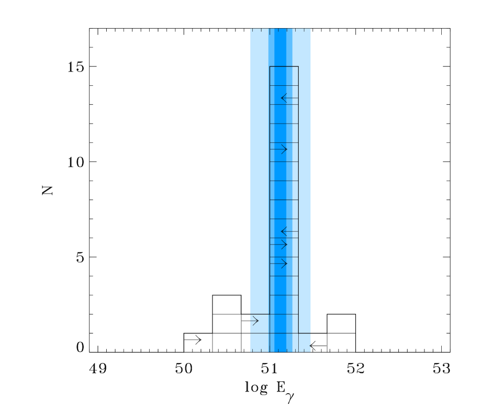
Figure 3: Distribution of the total energy $E_{\gamma}$ radiated in gamma-rays by GRBs, taking into account the jet opening angle inferred from the jet break time. From Bloom, Frail & Kulkarni (2003).

Frail et al. (2001) and Panaitescu & Kumar (2001) [see also Bloom, Frail & Kulkarni (2003)] find that most GRBs have a “standard” energy. That is, most GRBs have the same radiated energy, $E_{\gamma}=1.3\times 10^{51}$ ergs, to within a factor $\sim$ 2-3, if their isotropic equivalent energy is corrected for the jet opening angle $\theta_{\rm jet}$ inferred from the jet break time. This is illustrated in Figure 3, which shows the distribution of total radiated energies in gamma-rays $E_{\gamma}$ for 24 GRBs, after taking into account the jet opening angle inferred from the jet break time (Bloom, Frail & Kulkarni, 2003).

Pursuing this picture further, we show in Figure 4 the distribution of $E_{\rm iso}$, $L_{\rm iso}$, and $E_{\rm peak}$ as a function of $2\pi/\Omega_{\rm jet}$ for the HETE-2 and BeppoSAX GRBs with known redshifts. Figure 4 shows that all three quantities are strongly correlated with $\Omega_{\rm jet}$. The correlation between $E_{\rm iso}$ and $\Omega_{\rm jet}$ is implied by the fact that most GRBs have a standard energy (Frail et al., 2001; Panaitescu & Kumar, 2001). The correlation between $L_{\rm iso}$ and $\Omega_{\rm jet}$ is implied by the fact that most GRBs have a standard energy and the correlation between $E_{\rm iso}$ and $L_{\rm iso}$ (Lamb et al., 2004). The correlation between $E_{\rm peak}$ and $\Omega_{\rm jet}$ is implied by the fact that most GRBs have a standard energy, and the correlation between $E_{\rm iso}$ and $E_{\rm peak}$ found by Lloyd-Ronning, Petrosian & Mallozzi (2000) for BATSE bursts without redshifts and the tight relation between $E_{\rm iso}$ and $E_{\rm peak}$ found byAmati et al. (2002) for BeppoSAX bursts with known redshifts. Figure 4 demonstrates these three correlations directly.

The strength of the correlations of all three quantities with $\Omega_{\rm jet}$ lends additional support to a picture in which most GRB have a standard energy and the observed ranges of $\sim 10^{5}$ in $E_{\rm iso}$ and $L_{\rm iso}$ are due either to differences in the jet opening angle $\theta_{\rm jet}$ or to differences in the viewing angle $\theta_{\rm view}$ of the observer with respect to the axis of the jet. We pursue both of these possibilities below.

3 Jet Models of GRBs

Two phenomenological models of GRB jets have received widespread attention:

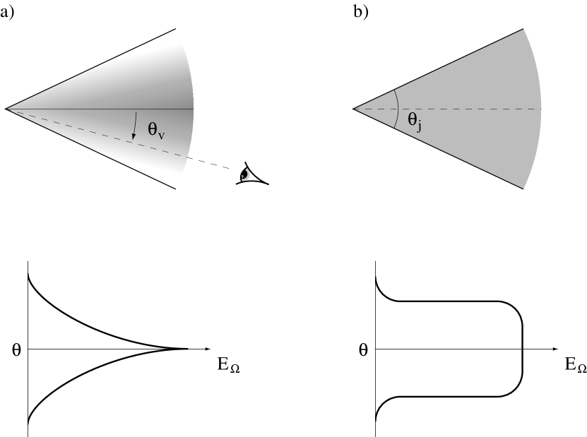
Figure 5: Schematic diagrams of the power-law universal and variable opening-angle jet models of GRBs from Ramirez-Ruiz & Lloyd-Ronning (2002). In the power-law universal jet model, the isotropic-equivalent energy and luminosity is assumed to decrease as the viewing angle $\theta_{\rm view}$ as measured from the jet axis increases. In order to recover the standard energy result (Frail et al., 2001), $E_{\rm iso}(\theta_{\rm view})\sim\theta_{\rm view}^{-2}$ is required. In the variable jet opening-angle model, GRBs produce jets with a large range of jet opening angles $\theta_{\rm jet}$. For $\theta_{\rm view}<\theta_{\rm jet}$, $E_{\rm iso}(\theta_{\rm view})\approx$ constant while for $\theta_{\rm view}>\theta_{\rm jet}$, $E_{\rm iso}(\theta_{\rm view})=0$. In this paper, we take $\theta_{\rm jet}$ to be the half-opening angle of the jet.

• The universal jet model (see the left-hand panel of Figure 5). In this model, all GRBs produce jets with the same structure (Rossi, Lazzati & Rees, 2002; Zhang & Mészáros, 2002; Mészáros, Ramirez-Ruiz, Rees & Zhang, 2002; Zhang, Woosley & Heger, 2004; Perna, Sari & Frail, 2003; Zhang et al., 2004). The energy $E_{\rm iso}$ and luminosity $L_{\rm iso}$ are assumed to decrease as the viewing angle $\theta_{\rm view}$ increases. The wide range of observed values of $E_{\rm iso}$ is then attributed to differences in the viewing angle $\theta_{\rm view}$. In order to recover the standard energy result (Frail et al., 2001; Panaitescu & Kumar, 2001; Bloom, Frail & Kulkarni, 2003) over a wide range in viewing angles, $E_{\rm iso}(\theta_{\rm view})\propto\theta_{\rm view}^{-2}$ is required (Rossi, Lazzati & Rees, 2002; Zhang & Mészáros, 2002).

• The variable jet opening-angle model (see the right-hand panel of Figure 5). In this model, GRB jets have a wide range of jet opening angles $\theta_{\rm jet}$ (Frail et al., 2001). For $\theta_{\rm view}<\theta_{\rm jet}$, $E_{\rm iso}(\theta_{\rm view})\approx$ constant, while for $\theta_{\rm view}>\theta_{\rm jet}$, $E_{\rm iso}(\theta_{\rm view})=0$. The wide range of observed values of $E_{\rm iso}$ is then attributed to differences in the jet opening angle $\theta_{\rm jet}$. This is the model that Frail et al. (2001) and Bloom, Frail & Kulkarni (2003) assume in deriving a standard energy for most bursts.

As described in the previous section, there is evidence that the relation between $E_{\rm iso}$ and $E_{\rm peak}$ extends over at least five decades in $E_{\rm iso}$, and appears to hold for XRFs and X-ray-rich GRBs, as well as for GRBs (Lamb et al., 2004); most bursts appear to have a standard energy (Frail et al., 2001; Panaitescu & Kumar, 2001; Bloom, Frail & Kulkarni, 2003); and there are correlations among $E_{\rm iso}$, $L_{\rm iso}$, and $E_{\rm peak}$, and between these quantities $\Omega_{\rm jet}$ (Frail et al., 2001; Bloom, Frail & Kulkarni, 2003; Lamb et al., 2004). Motivated by these results, we make three key assumptions in exploring a unified jet picture of all three kinds of bursts:

1. We assume that most XRFs, X-ray-rich GRBs, and GRBs have a standard energy $E_{\gamma}$ with a modest scatter.

2. We assume that, for most GRBs, $E_{\rm iso}$ and $E_{\rm peak}$ obey the relation (Lloyd-Ronning, Petrosian & Mallozzi, 2000; Amati et al., 2002; Lamb et al., 2004):

   $$E_{\rm peak}\propto(E_{\rm iso})^{1/2}\;,$$ (1)

   with a modest scatter, and that this relation holds for XRFs and X-ray-rich GRBs, as well as for GRBs.

3. We assume that the observed ranges of $\sim 10^{5}$ in $E_{\rm iso}$ and $L_{\rm iso}$ are due either to differences in the jet opening angle $\theta_{\rm jet}$ (in the variable jet opening-angle model) or to differences in the viewing angle $\theta_{\rm view}$ of the observer with respect to the axis of the jet (in the universal jet model).

4 Simulations of Observed Gamma-Ray Bursts

4.1 Overview of the Simulations

We begin by giving an overview of our population synthesis simulations of observed GRBs before describing the simulations in mathematical detail. Our overall approach is to simulate the GRBs that are observed by different instruments by (1) modeling the bursts in the source frame; (2) propagating the bursts from the source frame to us, using the cosmology that we have adopted; and (3) determining which bursts are observed and the properties of these bursts by modeling the instruments that observe them.

This logical sequence is evident in Figure 6, which shows a flowchart of the calculations involved in our simulations of bursts in the variable jet opening-angle model. For each simulated burst we obtain a redshift $z$ and a jet opening solid angle $\Omega_{\rm jet}$ by drawing from specific distributions. In addition, we introduce three lognormal smearing functions to generate a timescale $T$, a jet energy $E_{\gamma}$ and a coefficient for the $E_{\rm iso}-E_{\rm peak}$ relation ($C$). Using these five quantities, we calculate various rest-frame quantities ($E_{\rm iso}$, $L_{\rm iso}$, $E_{\rm peak}$, etc.). Finally, we construct a Band spectrum for each burst and transform it into the observer frame, which allows us to calculate fluences and peak fluxes, and to determine if the burst would be detected by various experiments.

Astronomical observations usually impose strong observational selection effects on the population of objects being observed. Consequently, the most rigorous approach to comparing models to data, and finding the best-fit parameters for these models, is to specify the models being compared, independent of any observations. This avoids the pitfall of circularity, in which the posited models are already distorted by strong observational selection effects. In practice, this approach is difficult to carry out, particularly when our understanding of the phenomenon of interest is quite limited, as is currently the case for GRB jets.

We therefore adopt an intermediate approach in this paper. We use those properties of GRBs that we have reason to believe are unlikely to be strongly affected by observational selection effects as a guide in specifying the models that we consider. We then extend the predictions of these models to regimes in which the observational selection effects are strong by modeling these effects in detail. We are then able to compare the predictions of the models with observations in the regimes where we believe observational selection effects are unlikely to be important and in the regimes where we know that observational selection effects are important.

4.2 GRB Rest-Frame Quantities

4.2.1 Variable Jet Opening-Angle Model

In this paper we investigate a variable jet opening-angle model in which the emissivity is a constant independent of the angle relative to the jet axis and the distribution of jet opening angles is a power law. In a subsequent paper, we investigate variable jet opening-angle models in which the emissivity is a constant independent of the angle relative to the jet axis and the distribution of jet opening angles is a Gaussian, and in which the emissivity is a Gaussian function of the angle relative to the jet axis and the distribution of jet opening angles is a power law (Donaghy, Graziani & Lamb, 2004a).

We assume that the emission from the jet is visible only when $\theta_{\rm view}<\theta_{\rm jet}$. In reality, emission from the jet may be seen when the observer is outside the opening angle of the jet, due to relativistic beaming effects. However, the angular width of the annulus within which the jet is visible (i.e., has a flux above some minimum observable flux) is small. If the opening angle of the jet is large (as is posited to be the case for XRFs in the variable jet opening angle model), the relative number of bursts that will be detectable because of relativistic beaming is therefore also small (Donaghy, 2004). If the opening angle of the jet is small (as is posited to be the case for GRBs in the variable jet opening angle model), the bulk $\Gamma$ in the jet may be large and the flux due to relativistic beaming that is seen by an observer outside the opening angle will then drop off precipitously. The relative number of bursts that will be detectable because of relativistic beaming is therefore again small (Donaghy, 2004).

The distribution in jet opening solid angle $\Omega_{\rm jet}$ then generates our GRB luminosity function; here we are primarily interested in a power-law distribution. We define the fraction of the sky subtended by the GRB jet to be

$$f_{\rm jet}=\frac{\Omega_{\rm jet}}{2\pi}=1-\cos\theta_{\rm jet}\;.$$ (2)

We define the true distribution of opening angles to be

$$P_{\rm true}(\Omega_{\rm jet})d\Omega_{\rm jet}={\rm const}\times(\Omega_{\rm jet})^{-\delta}d\Omega_{\rm jet}$$ (3)

over a range ($\Omega_{\rm jet}^{\rm min},\Omega_{\rm jet}^{\rm max}$). We define the observed distribution of opening angles to be

$$P_{\rm obs}(\Omega_{\rm jet})d\Omega_{\rm jet}={\rm const}\times(\Omega_{\rm jet})^{-\delta_{\rm sim}}d\Omega_{\rm jet}\propto f_{\rm jet}^{-\delta_{\rm sim}}.$$ (4)

Since we can observe only those bursts whose jets are oriented toward the Earth, the distribution of opening angles of observable bursts is related to the true distribution of opening angles by

$$P_{\rm obs}(\Omega_{\rm jet})=f_{\rm jet}P_{\rm true}(\Omega_{\rm jet})\propto(\Omega_{\rm jet})^{(1-\delta)}$$ (5)

We thus simulate bursts using the power-law index $\delta_{\rm sim}$ from which the true power-law index can be found using the relation $\delta=1+\delta_{\rm sim}$.

The isotropic-equivalent emitted energy $E_{\rm iso}$ is then given by

$$E_{\rm iso}=\frac{E_{\gamma}}{f_{\rm jet}}=\frac{E_{\gamma}}{(\Omega_{\rm jet}/2\pi)},$$ (6)

where $E_{\gamma}$ is the total radiated energy of the burst. Using a full maximum likelihood approach, we reproduce the parameters of the lognormal distribution derived by Bloom, Frail & Kulkarni (2003), using their sample of GRBs with observed jet break times (see Figure 7). We find no evidence for any correlation of $E_{\gamma}$ with redshift (see again Figure 7). We therefore draw values for $E_{\gamma}$ randomly from the narrow lognormal distribution defined by

$$G(E_{\gamma})d\log E_{\gamma}=\exp\left(\frac{-(\log E_{\gamma}-\log E_{\gamma}^{0})^{2}}{2\sigma_{E}^{2}}\right)d\log E_{\gamma}\;,$$ (7)

where $\log E_{\gamma}^{0}({\rm erg})=51.070$ and $\log\sigma_{E}=0.35$ (see also Table 1).

Our simulations thus use a value $E_{\gamma}^{0}=1.17\times 10^{51}\ {\rm ergs}$, which is fully consistent with the value $E_{\gamma}^{0}=1.33\times 10^{51}\ {\rm ergs}$ found by Bloom, Frail & Kulkarni (2003). However, the Bloom, Frail and Kulkarni sample of GRBs contained no XRFs. The values of $E_{\rm iso}$ for XRFs 020903 (Sakamoto et al., 2004a) and 030723 (Lamb et al., 2004) are $\sim 100$ times lower than the value of $E_{\gamma}$ derived by Frail et al. (2001) and Bloom, Frail & Kulkarni (2003). Thus there is no value of the opening solid angle $\Omega_{\rm jet}$ that can accommodate these values of $E_{\rm iso}$. Since we are pursuing a unified jet model of XRFs, X-ray-rich GRBs, and GRBs, we must be able to accommodate values of $E_{\rm iso}$ that are $\sim 100$ times less than the value of $E_{\gamma}$ derived by Frail et al. (2001) and Bloom, Frail & Kulkarni (2003).

We therefore introduce the ability to rescale $\log E_{\gamma}^{0}$, the central value of $E_{\gamma}$. This is equivalent to rescaling the range of $\Omega_{\rm jet}$, since only $E_{\rm iso}$ is observed. In doing so, we note that the derivation of $E_{\gamma}$ is dependent on the coefficient in front of the relation between the jet-break time and $\theta_{\rm jet}$, and that the value of this coefficient is uncertain by a factor 4-5 (Rhoads, 1999; Sari, Piran & Halpern, 1999).

This rescaling of $E_{\gamma}$ introduces an additional parameter $C_{\rm jet}$ into our model:

$$E_{\rm iso}=\frac{E_{\gamma}}{C_{\rm jet}\cdot\Omega_{\rm jet}/2\pi}.$$ (8)

XRF 020903, the dimmest burst in our sample, has $E_{\rm iso}=2.3\times 10^{49}\ {\rm ergs}$ (Sakamoto et al., 2004a). Accounting for this burst requires that $C_{\rm jet}$ be at least $57.8$; this choice is conservative in the sense that it implies that XRF 020903 lies at the faintest end of the range of possible values of $E_{\rm iso}$ and has the maximum possible opening angle of $\Omega_{\rm jet}=2\pi$. The brightest burst in our sample is GRB 990123, which has $E_{\rm iso}=2.8\times 10^{54}\ {\rm ergs}$. Thus the range of $E_{\rm iso}$ is at least $\sim 10^{5}$, and so the range of $\Omega_{\rm jet}$ must also be $\sim 10^{5}$. Since only $E_{\rm iso}$ is a directly observable quantity, the value of $C_{\rm jet}$ is degenerate with the value of the jet opening solid angle $\Omega_{\rm jet}$. Thus GRB 990123 provides a constraint only on $C_{\rm jet}\cdot\Omega_{\rm jet}^{\rm min}$.

Since we wish our burst simulations to explain the full range of observed $E_{\rm iso}$, we require a range of approximately five decades in $\Omega_{\rm jet}$ (conservatively, from $2\pi$ to $2\pi\times 10^{-5}\ {\rm sr}$). We have then varied $C_{\rm jet}$ to best match the observed cumulative distributions shown in Figure 14, as determined by visual comparison of the observed and predicted cumulative distributions. The fiducial model that we use in this paper has a value of $C_{\rm jet}=95$. This gives minimum and maximum values of $E_{\rm iso}$ of $1.4\times 10^{49}\ {\rm ergs}$ and $1.4\times 10^{54}\ {\rm ergs}$. The former value of $E_{\rm iso}$ implies a jet opening angle $\theta_{\rm jet}=67^{\circ}$ for XRF 020903 (the burst with the smallest value of $E_{\rm iso}$ in our sample). The latter value of $E_{\rm iso}$ is slightly smaller than the value of $E_{\rm iso}$ for GRB 990123 (the burst with the largest value of $E_{\rm iso}$ in our sample), but the range of simulated $E_{\gamma}$ values, although narrow, is sufficient to account for this event and events like it. We have used the value $C_{\rm jet}=95$ to rescale the $\Omega_{\rm jet}$ values reported by Bloom, Frail & Kulkarni (2003) (see Figure 12); this corresponds to making the coefficient in the relation between the jet break time and $\theta_{\rm jet}$ a factor of $\sim 10$ smaller, and therefore the value of $\theta_{\rm jet}$ a factor of $\sim 10$ smaller.

Thus the value of $C_{\rm jet}$ that we adopt in this paper requires that the value of $\theta_{\rm jet}$ corresponding to a given jet break time be smaller than the value that is typically assumed by a factor of about ten; i.e., a factor of two more than the uncertainty stated by Sari, Piran & Halpern (1999). We return to this point below in the Discussion section.

We incorporate the relation between $E_{\rm iso}$ and $E_{\rm peak}$ found by Amati et al. (2002) and extended by Lamb et al. (2004), using a second narrow lognormal distribution, defined by

$$E_{\rm peak}=C\cdot\left(\frac{E_{\rm iso}}{10^{52}\ {\rm erg}}\right)^{s}\;,$$ (9)

and

$$G(C)d\log C=\exp\left(\frac{-(\log C-\log C_{0})^{2}}{2\sigma_{C}^{2}}\right)d\log C.$$ (10)

We set the power-law index $s=0.5$. Then, using a full maximum likelihood approach to fit these equations to the HETE-2 and BeppoSAX GRBs with known redshifts (see Figures 2 and 7), we find maximum likelihood best-fit parameters $C_{0}=90.4$ keV and $\sigma_{C}=0.70$ (see also Table 1). Again we find no evidence for any correlation of $C$ with redshift (see Figure 7). We therefore draw randomly from this Gaussian distribution to choose the value of $E_{\rm peak}$ corresponding to the value of $E_{\rm iso}$ for a particular burst.

Finally, we require the timescale that converts the isotropic-equivalent energy $E_{\rm iso}$ of a burst to the isotropic-equivalent peak luminosity $L_{\rm iso}$ of a burst. Using a full maximum likelihood approach, we determine this timescale by fitting a third narrow lognormal distribution, defined by

$$G(T)d\log T=\exp\left(\frac{-(\log T-\log T_{0})^{2}}{2\sigma_{T}^{2}}\right)d\log T\;,$$ (11)

to the distribution of the ratio $E_{\rm iso}$/$L_{\gamma}$ for the HETE-2 and BeppoSAX bursts with known redshifts (see Figure 7). Thus the timescale $T$ is defined in the rest frame of the GRB source. We find maximum likelihood best-fit parameters $T_{0}=3.41$ sec and $\sigma_{T}=0.33$ (see also Table 1). Again, we find no evidence for any correlation of $T$ with redshift (see Figure 7). We therefore draw randomly from this Gaussian distribution and use the formula $L_{\rm iso}=E_{\rm iso}/T$ to convert $E_{\rm iso}$ to $L_{\rm iso}$, and thus also to convert burst fluences to peak fluxes. We note that the sample used for this fit also contains no XRFs.

4.2.2 Power-Law Universal Jet Model

In order to recover the standard energy result in the universal jet model requires $E_{\rm iso}\propto\theta_{\rm view}^{-2}$ (Rossi, Lazzati & Rees, 2002; Zhang & Mészáros, 2002; Perna, Sari & Frail, 2003). Therefore in this paper we investigate a universal jet model in which the emissivity is a power-law function of the angle relative to the jet axis. In a subsequent paper (Donaghy, Graziani & Lamb, 2004a), we investigate a universal jet model in which the emissivity is a Gaussian function of the angle relative to the jet axis (Zhang et al., 2004)).

The requirement $E_{\rm iso}\propto\theta_{\rm view}^{-2}\propto\Omega_{\rm view}^{-1}$ allows us to simulate the power-law universal jet model by simply making the substitution $\Omega_{\rm jet}\to\Omega_{\rm view}$ in the variable jet opening-angle simulations. To see this, compare Equation 6 with the relation:

$$E_{\rm iso}\propto\frac{1}{\theta_{\rm view}^{2}}\propto\frac{1}{\Omega_{\rm view}}.$$ (12)

Although the physical interpretations of the two equations are entirely different, they give the same results. In addition to this substitution, we have to specify $\delta_{\rm sim}$ for the power-law universal jet model. Since the bursts are randomly oriented with respect to our line of sight, we draw $\Omega_{\rm view}$ values from a flat distribution, $d\Omega_{\rm view}$, which corresponds to $\delta_{\rm sim}=0$. Drawing from this distribution results in very few small $\theta_{\rm view}$ values compared to the very large number of $\theta_{\rm view}$ values near $\theta_{\rm view,max}$ (the angular extent of the universal jet) or $90^{\circ}$, whichever is smaller. Therefore, in this model, most bursts have $\theta_{\rm view}\sim\theta_{\rm view,max}$ or $90^{\circ}$, whichever is smaller; and the range of observed $\Omega_{\rm view}$ values in logarithmic space is small for a finite sample of bursts. As a result, the power-law universal jet model predicts that most of the bursts arriving at the Earth will have small values of $E_{\rm iso}$, $L_{\rm iso}$, etc. (Rossi, Lazzati & Rees, 2002; Perna, Sari & Frail, 2003).

We also introduce the ability to rescale the central value of $E_{\gamma}$ in the power-law universal jet model (see Equation 8). For this model we consider two cases: in the first case, we “pin” the minimum value of $E_{\rm iso}$ (i.e., the value of $E_{\rm iso}$ corresponding to $\Omega_{\rm view}=2\pi$) to the value of $E_{\rm iso}$ for XRF 020903; in the second case, we pin the minimum value of $E_{\rm iso}$ to the value of $E_{\rm iso}$ for GRB 980326 (the smallest $E_{\rm iso}$ in our sample of HETE-2 and BeppoSAX bursts with known redshifts, apart from the XRFs). In the first case, we derive $C_{\rm jet}=58$, and in the second $C_{\rm jet}=0.24$. In the first case, the power-law universal jet model can then generate the full observed range of $E_{\rm iso}$ (i.e., both XRFs and GRBs), while in the second case, it can generate the range of $E_{\rm iso}$ values corresponding to GRBs, but not to XRFs or X-ray-rich GRBs.

4.3 Gamma-Ray Burst Rate as a Function of Redshift

The observed rate of GRBs per redshift interval $dz$ is given by

$$\rho(z)=R_{GRB}(z)\times(1+z)^{-1}\times 4\pi r(z)^{2}\frac{dr}{dz}=\left[\rm\frac{num}{dz\cdot year}\right]\;,$$ (13)

where $R_{GRB}(z)$ is the rate of GRBs per comoving volume and $r(z)$ is the comoving distance to the source [see §4.3 below for the precise definition of $r(z)$]. We use the phenomenological parameterization of the star-formation rate (SFR) as a function of redshift suggested by Rowan-Robinson (2001) to parameterize the GRB rate as a function of redshift. In this parameterization, $R_{GRB}$ is given by

$$R_{GRB}(z)=R_{0}\,\left(\frac{t(z)}{t(0)}\right)^{P}\exp\left[Q\left(1-\frac{t(z)}{t(0)}\right)\right]=\left[\rm\frac{num}{year\cdot Gpc^{3}}\right].$$ (14)

Here, $t(z)$ is the elapsed coordinate time since the big bang at that redshift. In this paper, we adopt the values $P=1.2$ and $Q=5.4$, which provide a good fit to existing data on the star-formation rate (SFR) as a function of redshift. The resulting curve of the SFR as a function of redshift is given in Figure 8. It rises rapidly from $z=0$, peaks at $z\approx 1.5$, and then decreases gradually with increasing redshift. We draw GRB redshifts randomly from this SFR curve.

The actual SFR as a function of redshift is uncertain, and the GRB rate as a function of redshift is even more uncertain. Several studies have suggested that the GRB rate may be flat, or may even increase, at high redshifts (Fenimore & Ramirez-Ruiz, 2000; Lloyd-Ronning, Fryer & Ramirez-Ruiz, 2002; Reichart & Lamb, 2001). The particular choice that we have made of the GRB rate as a function of redshift has little effect on the comparisons with observations that we carry out in this paper, since all of the bursts that we consider are at modest redshifts ($z\lesssim 3$). However, predictions of the fraction of bursts that lie at very high redshifts ($z>5$), and therefore the number of detectable bursts at very high redshifts, are sensitive to the shape of the GRB rate curve at very high redshifts.

4.4 Cosmology

The Rowan-Robinson SFR model depends on a few basic cosmological parameters, as do the observed peak photon number and energy fluxes and fluences of the bursts. In this paper, we adopt the values $\Omega_{M}=0.3$, $\Omega_{\Lambda}=0.7$ and $H_{0}=65$ km s^-1 Mpc^-1.

The comoving distance to redshift $z$ is defined by

$$\frac{dr}{dz}=\frac{c}{H_{0}}\left[\Omega_{k}(1+z)^{2}+\Omega_{\Lambda}+\Omega_{M}(1+z)^{3}+\Omega_{R}(1+z)^{4}\right]^{-1/2},$$ (15)

and integrating this equation over $dz$ gives us $r(z)$.

To calculate the time since the big-bang we integrate the following formula:

$$dt=\frac{da}{a\,H_{0}}\left[\Omega_{k}a^{-2}+\Omega_{\Lambda}+\Omega_{M}a^{-3}+\Omega_{R}a^{-4}\right]^{-1/2},$$ (16)

which yields an expression for $t(z)$. Here $a=(1+z)^{-1}$. For our adopted cosmology, there is an analytic expression for $t(z)$, which is

$$H_{0}t(z)=\frac{2}{3\Omega_{\Lambda}^{1/2}}\sinh^{-1}\left[\left(\frac{\Omega_{\Lambda}}{\Omega_{M}}\right)^{1/2}(1+z)^{-3/2}\right]\;,$$ (17)

but there is no analytic expression for $r(z)$.

4.5 Observable Quantities

In this paper, we assume that the spectra of GRBs are a Band function (Band, et al., 1993) in which $\alpha=-1$, $\beta=-2.5$ and $E^{\rm obs}_{\rm peak}=E_{\rm peak}/(1+z)$. We have also done simulations assuming $\alpha=-0.5$ and -1.5, and $\beta=-2.0$ and -3.0; these different choices make little difference in our results.

Given $E_{\rm iso}$, $E_{\rm peak}$, and $T$, we calculate $L_{\rm iso}^{E}=E_{\rm iso}/T$ and the normalization constant $A$ of the Band spectrum in the rest frame of the burst source. We can then calculate the following peak fluxes and fluences:

$$F^{\rm P}_{E}=\frac{L_{\rm iso}^{E}}{4\pi r^{2}(z)(1+z)^{2}}=[\rm erg\;cm^{-2}\;s^{-1}]\;;\;\;\;\;\;\;\;\;\;S_{E}=F^{\rm P}_{E}\cdot T\cdot(1+z)=[\rm erg\;cm^{-2}]\;;$$ (18)

$$F^{\rm P}_{N}=\frac{L_{\rm iso}^{N}}{4\pi r^{2}(z)(1+z)}=[\rm phot\;cm^{-2}\;s^{-1}]\;;\;\;\;\;\;\;\;\;\;S_{N}=F^{\rm P}_{N}\cdot T\cdot(1+z)=[\rm phot\;cm^{-2}]\;.$$ (19)

However, these are bolometric quantities, not observed quantities; in order to calculate the observed peak fluxes and fluences, we must model the instruments.

Given $E_{\rm iso}$, $E_{\rm peak}$, and $z$ from the simulations, we calculate the normalization constant $A^{*}$ of the Band function by considering the bolometric fluence as observed in our reference frame.

$$S_{E}^{\rm bol}=\frac{E_{\rm iso}}{4\pi(1+z)r(z)^{2}}=A^{*}\times\int_{0}^{\infty}\,EN(E;\alpha,\beta,E^{\rm obs}_{\rm peak},A=1)\,dE$$ (20)

Once we have $A^{*}$, we can calculate the observed fluxes and fluences in the passband of our instrument,

$$S_{E}^{\rm obs}=\int_{\rm instr}\,EN(E;\alpha,\beta,E^{\rm obs}_{\rm peak},A^{*})\,dE\;;\;\;\;\;\;\;\;\;\;F_{E}^{P,{\rm obs}}=\frac{S_{E}^{obs}}{T(1+z)}\;;$$ (21)

$$S_{N}^{\rm obs}=\int_{instr}\,N(E;\alpha,\beta,E^{\rm obs}_{\rm peak},A^{*})\,dE\;;\;\;\;\;\;\;\;\;\;F_{N}^{P,{\rm obs}}=\frac{S_{N}^{obs}}{T(1+z)}\;.$$ (22)

To determine whether a particular burst will be detected by a particular instrument, we define the efficiency as a function of $E^{\rm obs}_{\rm peak}$,

$$\epsilon(E^{\rm obs}_{\rm peak})=\frac{\int_{\rm instr}\,N(E;\alpha,\beta,E^{\rm obs}_{\rm peak},A^{*})\,dE}{\int_{0.1}^{10000}\,N(E;\alpha,\beta,E^{\rm obs}_{\rm peak},A^{*})\,dE}=\frac{F_{N}^{P,{\rm inst}}}{F_{N}^{P,\oplus}}\;,$$ (23)

where $F_{N}^{P,\oplus}$ and $F_{N}^{P,{\rm inst}}$ are the bolometric peak photon number flux of the burst at the Earth and the peak photon number flux of the burst as measured by a particular instrument, respectively. This expression gives a shape function which we normalize to Figures 2 through 9 of Band (2003) for the desired detector. Note that our shape function is the same as Band’s, except that we consider incident burst spectra extending from 0.1 - 10,000 keV instead of from 1 - 1000 keV, in order to encompass the full range of values of $E^{\rm obs}_{\rm peak}$ observed by HETE-2 for XRFs, X-ray-rich GRBs, and GRBs.

The normalization is approximately given by

$$D_{inst}=\frac{C_{\rm min}(\sigma,B)}{A_{\rm eff}\cdot\Delta t_{\rm trig}}=[\rm phot\;s^{-1}\;cm^{-2}]\;,$$ (24)

where $C_{\rm min}(\sigma,B)$ is the minimum detectable number of counts in the detector, $\sigma$ is the SNR required for detection, $B$ is the background count rate from the diffuse X-ray background, $A_{\rm eff}$ is the effective area of the detector, and $\Delta t_{\rm trig}$ is the trigger timescale (Band, 2003). A burst is detected if

$$F_{N}^{P,\oplus}\geq\frac{D_{\rm inst}}{\epsilon(E^{\rm obs}_{\rm peak})}=F_{N,{\rm min}}^{P,\oplus}\;;{\rm\ i.e.,}\;\;F_{N}^{P,{\rm inst}}\geq D_{\rm inst}=F_{N,{\rm min}}^{P,{\rm inst}}\;.$$ (25)

Thus $D_{\rm inst}$ is the peak number flux detection threshold in the instrument passband.

We have reproduced the results of Band (2003) for BATSE on CGRO, the WFC and GRBM on BeppoSAX , and the WXM and FREGATE on HETE-2. However, we use a trigger timescale $\Delta t_{\rm trig}=5$ seconds for the WXM on HETE-2, rather than the value of 1 second used by Band (2003). We also use a threshold SNR for detection of a burst by the GRBM on BeppoSAX of 15 (Costa & Frontera, 2003), rather than the value of $5.6$ used by Band (2003).

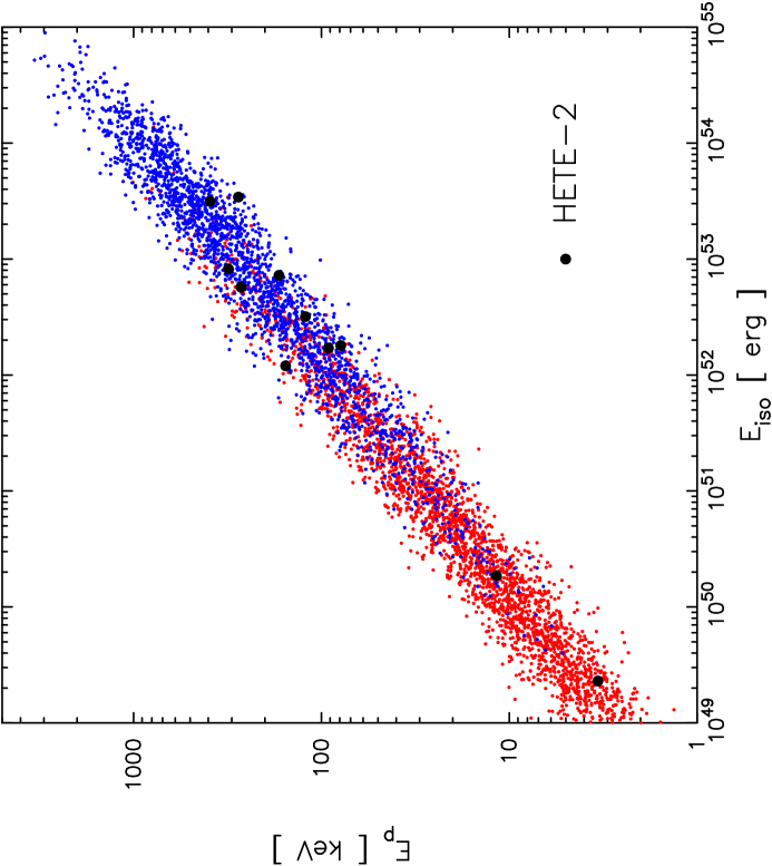
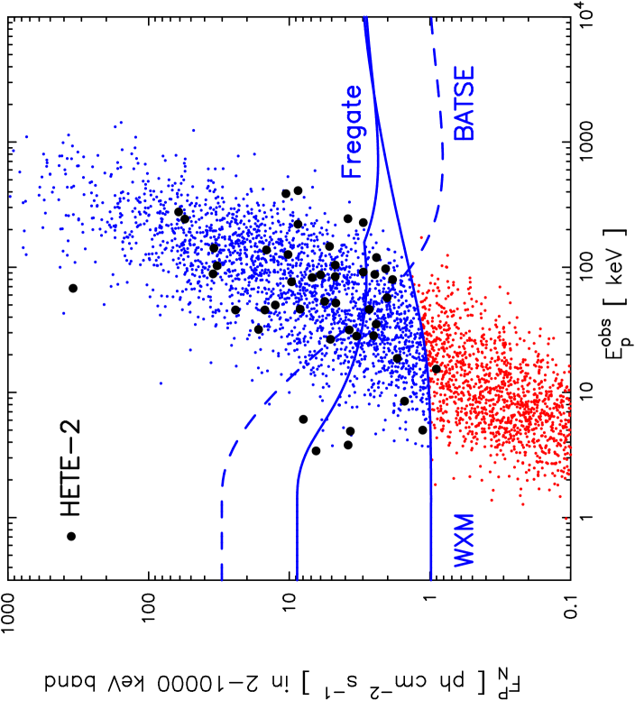
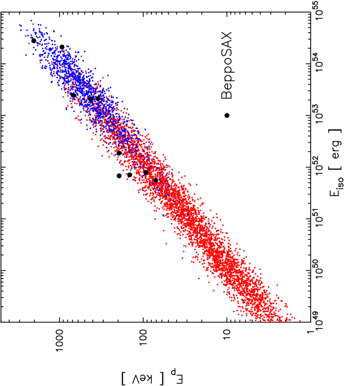
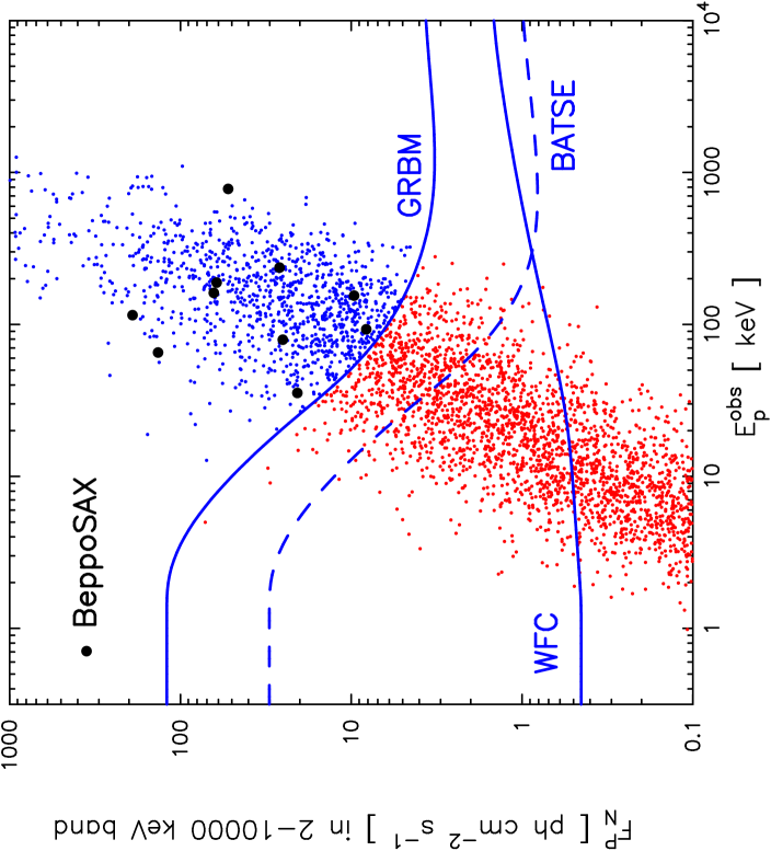
Figure 9: Comparison of the detectability of bursts by HETE-2 and BeppoSAX in the variable jet opening-angle model for $\delta=2$. Detected bursts are shown in blue and non-detected bursts in red. The left-hand panels show bursts in the [$E_{\rm iso},E_{\rm peak}$]-plane detected by HETE-2 (upper panel) and by BeppoSAX (lower panel). For each experiment, we overplot the locations of the HETE-2 and BeppoSAX bursts with known redshifts. The observed burst in the lower left-hand corner of the HETE-2 panel is XRF 020903, the most extreme burst in our sample. The agreement between the observed and predicted distributions of bursts is good. The right-hand panels show bursts in the [$E^{\rm obs}_{\rm peak},F^{\rm P}_{N}(2-10000\ {\rm keV})$]-plane detected by HETE-2 (upper panel) and by BeppoSAX (lower panel). For each experiment we show the sensitivity thresholds for their respective instruments plotted as solid blue lines. The BATSE threshold is shown in both panels as a dashed blue line. Again, the agreement between the observed and predicted distributions of bursts is good. The left-hand panels exhibit the constant density of bursts per logarithmic interval in $E_{\rm iso}$ and $E_{\rm peak}$ given by the variable jet opening-angle model for $\delta=2$.

Figure 9 shows the threshold sensitivity curves in peak photon number flux $F^{\rm P}_{N}$ for the WXM and FREGATE on HETE-2 and for the WFC and GRBM on BeppoSAX as a function of $E^{\rm obs}_{\rm peak}$, the observed peak energy of the $\nu F_{\nu}$ spectrum of the burst. Since BeppoSAX could not trigger on WFC data and was forced to rely on the less-sensitive GRBM for its triggers, we consider a burst to have been detected by BeppoSAX only if its peak flux falls above the GRBM sensitivity threshold. Since HETE-2 can trigger on WXM data, we consider a burst to have been detected if its peak flux falls above the minimum of the WXM and FREGATE sensitivity thresholds. These bursts form the ensemble of observed bursts from which we construct various observed distributions.

5 Results

In comparing the observed properties of XRFs, X-ray-rich GRBs, and GRBs, and their predicted properties in the variable jet opening-angle model, we consider values of the power-law index for the distribution of jet solid angles $\Omega_{\rm jet}$ of $\delta$ = 1, 2, and 3. As we will see, the observed properties of the bursts are fit best by $\delta=2$, which implies approximately equal numbers of bursts per logarithmic interval in all observed quantities.

In comparing the observed properties of XRFs, X-ray-rich GRBs, and GRBs, and their predicted properties in the power-law universal jet model, we adopt $E_{\rm iso}\propto\Omega_{\rm view}^{-1}$ since this relation is required in order to recover the standard energy result for GRBs. In addition, we consider two possibilities for the range of $\Omega_{\rm view}$. In the first case, we require the power-law universal jet model to account for the full range of the $E_{\rm iso}-E_{\rm peak}$ relation, including XRFs, X-ray-rich GRBs, and GRBs; i.e., we fix the normalization of $E_{\gamma}^{0}$ so that the smallest value of $E_{\rm iso}$ given by the model is the value of $E_{\rm iso}$ for XRF 020903. In the second case, we fix the normalization of $E_{\gamma}^{0}$ so that the smallest value of $E_{\rm iso}$ given by the model is the $E_{\rm iso}$ value for GRB 980326, the GRB with the smallest $E_{\rm iso}$ in the BeppoSAX sample.

The data sets for $S_{E}$ and $E^{\rm obs}_{\rm peak}$, and especially for $E_{\rm iso}$ and $E_{\rm peak}$ (which require knowledge of the redshift of the burst), are sparse at the present time. The latter two data sets also suffer from a large observational selection effect (there is a dearth of XRFs with known redshifts because the X-ray and optical afterglows of XRFs are so faint). In addition, the KS test (which is the appropriate test to use to compare cumulative distributions) is notoriously weak. We therefore do not think that it is justified to carry out detailed fits to these data sets at this time – in fact we think that doing so is likely to produce highly misleading results. We have therefore contented ourselves with making fits to these data sets “by eye,” which can support qualitative – but not quantitative – conclusions.

Figure 9 shows the detectability of bursts by HETE-2 and BeppoSAX in the variable jet opening-angle model for $\delta=2$. Detected bursts are shown in blue and non-detected bursts in red. The left-hand panels show bursts in the [$E_{\rm iso},E_{\rm peak}$]-plane detected by HETE-2 (upper panel) and by BeppoSAX (lower panel). For each experiment, we overplot the locations of the HETE-2 and BeppoSAX bursts with known redshifts. The observed burst in the lower left-hand corner of the HETE-2 panel is XRF 020903, the most extreme burst in our sample. The agreement between the observed and predicted distributions of bursts is good. The right-hand panels show bursts in the [$E^{\rm obs}_{\rm peak},F^{\rm P}_{N}(0.1-10000\ {\rm keV})$]-plane detected by HETE-2 (upper panel) and by BeppoSAX (lower panel). For each experiment we show the sensitivity thresholds for their respective instruments plotted in solid blue. The BATSE threshold is shown in both panels as a dashed blue line. Again, the agreement between the observed and predicted distributions of bursts is good. The left-hand panels exhibit the constant density of bursts per logarithmic interval in $E_{\rm iso}$ and $E_{\rm peak}$ given by the variable jet opening-angle model for $\delta=2$. Since $L_{\rm iso}=E_{\rm iso}/T$, this choice of $\delta=2$ corresponds to a GRB luminosity function $f(L_{\rm iso})\propto L_{\rm iso}^{-1}$, which is roughly consistent with those found by Schmidt (2001) and Lloyd-Ronning, Fryer & Ramirez-Ruiz (2002).

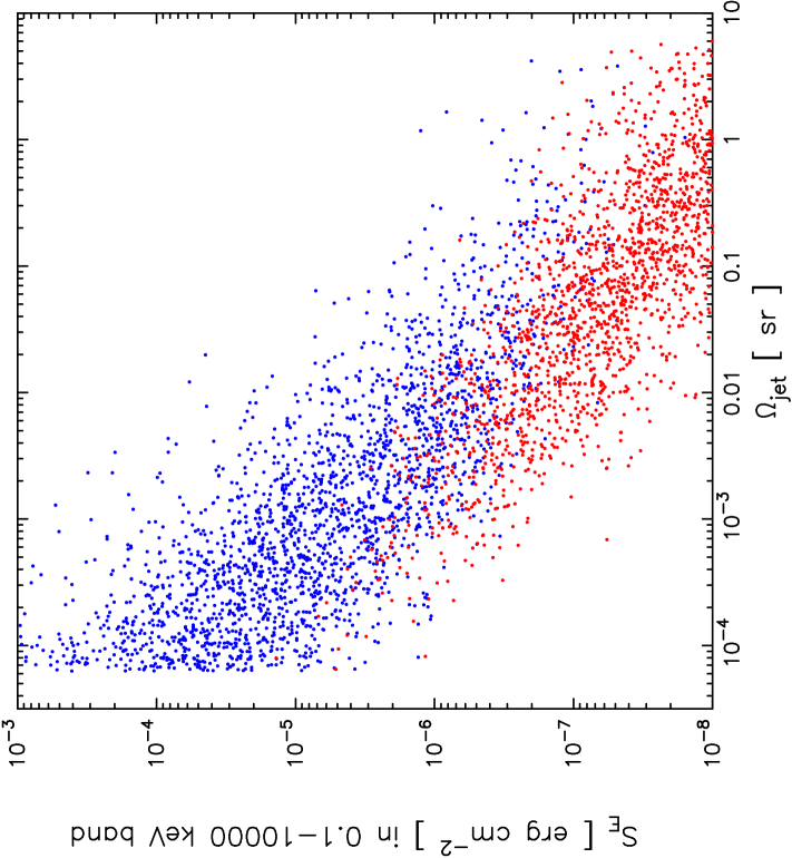
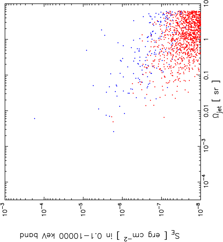
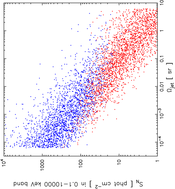
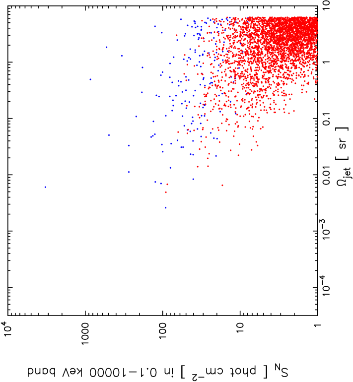
Figure 10: Scatter plots of $S_{E}$ and $S_{N}$ versus $\Omega_{\rm jet}$. The top panels show the predicted distributions in the variable jet opening-angle model for $\delta=2$, while the bottom panels show the power-law universal jet model pinned to the $E_{\rm iso}$ value of XRF 020903 (see text). Bursts detected by the WXM are shown in blue and non-detected bursts in red. The top panels exhibit the constant density of bursts per logarithmic interval in $S_{E}$, $S_{N}$, and $\Omega_{\rm jet}$ given by the variable jet opening-angle model for $\delta=2$. The bottom panels exhibit the concentration of bursts at $\Omega_{\rm jet}\equiv\Omega_{\rm view}\approx 2\pi$ and the resulting preponderance of XRFs relative to GRBs in the power-law universal jet model when it is pinned to the $E_{\rm iso}$ value of XRF 020903; i.e., when one attempts to extend the model to include XRFs and X-ray-rich GRBs, as well as GRBs.

Figure 10 shows scatter plots of $S_{E}$ and $S_{N}$ versus $\Omega_{\rm jet}$. The top panels show the predicted distributions in the variable jet model for $\delta=2$, while the bottom panels show the power-law universal jet opening-angle model pinned to the $E_{\rm iso}$ value of XRF 020903. Detected bursts are shown in blue and non-detected bursts in red. The top panels exhibit the constant density of bursts per logarithmic interval in $S_{E}$, $S_{N}$, and $\Omega_{\rm jet}$ given by the variable jet opening-angle model for $\delta=2$. The bottom panels exhibit the concentration of bursts at $\Omega_{\rm jet}\equiv\Omega_{\rm view}\approx 2\pi$ and the resulting preponderance of XRFs relative to GRBs in the power-law universal jet model when it is pinned to the $E_{\rm iso}$ value of XRF 020903; i.e., when one attempts to extend the model to include XRFs and X-ray-rich GRBs, as well as GRBs.

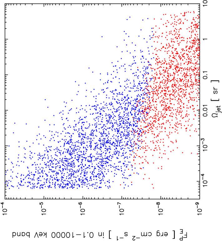
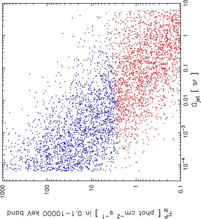
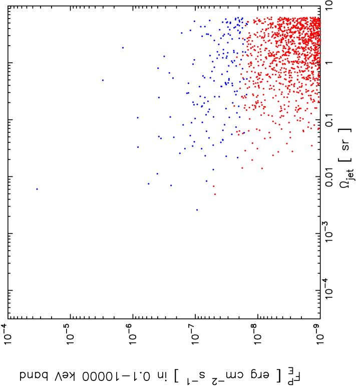
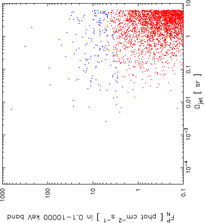
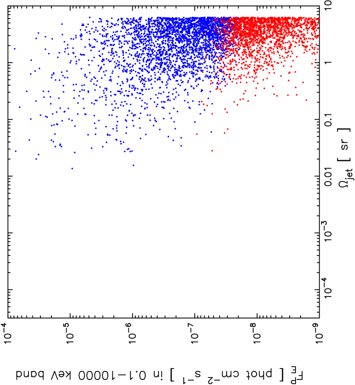
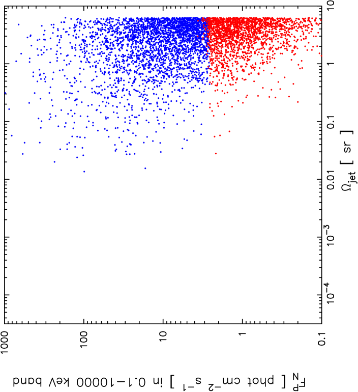
Figure 11: Scatter plots of $F^{\rm P}_{E}$ and $F^{\rm P}_{N}$ versus $\Omega_{\rm jet}$. The top panels show the predicted distributions in the variable jet opening-angle model for $\delta=2$, while the middle and the bottom panels show the power-law universal jet model pinned to the $E_{\rm iso}$ values of XRF 020903 and GRB 980326, respectively (see text). Bursts detected by the WXM are shown in blue and non-detected bursts in red.

Figure 11 shows scatter plots of $F^{\rm P}_{E}$ and $F^{\rm P}_{N}$ versus $\Omega_{\rm jet}$. The top panels show the predicted distributions in the variable jet opening-angle model for $\delta=2$, while the middle and the bottom panels show the power-law universal jet model pinned to the $E_{\rm iso}$ values of XRF 020903 and GRB 980326, respectively. In these scatter plots, as in the other scatter plots presented in this paper, we show a random subsample (usually 5000 bursts) of the 50,000 bursts that we have generated. Detected bursts are shown in blue and non-detected bursts in red. The top panels exhibit the constant density of bursts per logarithmic interval in $F^{\rm P}_{E}$, $F^{\rm P}_{N}$, and $\Omega_{\rm jet}$ given by the variable jet opening-angle model for $\delta=2$. The middle and bottom panels show the concentration of bursts at $\Omega_{\rm jet}\equiv\Omega_{\rm view}\approx 2\pi$. The middle panels show the resulting preponderance of XRFs relative to GRBs in the power-law universal jet model when it is pinned to the $E_{\rm iso}$ values of XRF 020903; i.e., when one attempts to extend the model to include XRFs and X-ray-rich GRBs, as well as GRBs.

Figure 12 shows the observed and predicted cumulative distributions of $\Omega_{\rm jet}$. The left panel shows the cumulative distributions of $\Omega_{\rm jet}$ predicted by the variable jet opening-angle model for $\delta=1$, $2$ and $3$ (solid curves), compared to the observed cumulative distribution of the values of $\Omega_{\rm jet}$ given in Bloom, Frail & Kulkarni (2003) scaled downward by a factor of $C_{\rm jet}$ = 95 (solid histogram). The predicted cumulative distribution of $\Omega_{\rm jet}$ given by $\delta=2$ fits the the shape and values of the scaled $\Omega_{\rm jet}$ distribution reasonably well. The right panel shows the cumulative $\Omega_{\rm jet}\equiv\Omega_{\rm view}$ distributions predicted by the power-law universal jet model with the minimum value of $E_{\rm iso}$ pinned to the value of $E_{\rm iso}$ for XRF 020903 (solid curve) and to the value of $E_{\rm iso}$ for GRB 980326 (dashed curve) These models are compared with the observed cumulative distribution of the values of $\Omega_{\rm jet}$ given in Bloom, Frail & Kulkarni (2003) (dashed histogram) and the same distribution scaled downward by a factor of $C_{\rm jet}$ = 95 (solid histogram). The cumulative $\Omega_{\rm jet}$ distribution predicted by the power-law universal jet model pinned to GRB 9980326 fits the shape and values of the observed cumulative distribution given by the values of $\Omega_{\rm jet}$ in Bloom, Frail & Kulkarni (2003) reasonably well if the observed values are scaled upward by a factor of $\approx$ 7. The cumulative distribution of $\Omega_{\rm jet}$ predicted by the power-law universal jet model pinned to XRF 020903 does not fit the shape of the observed cumulative distribution of $\Omega_{\rm jet}$ for any scaling factor.

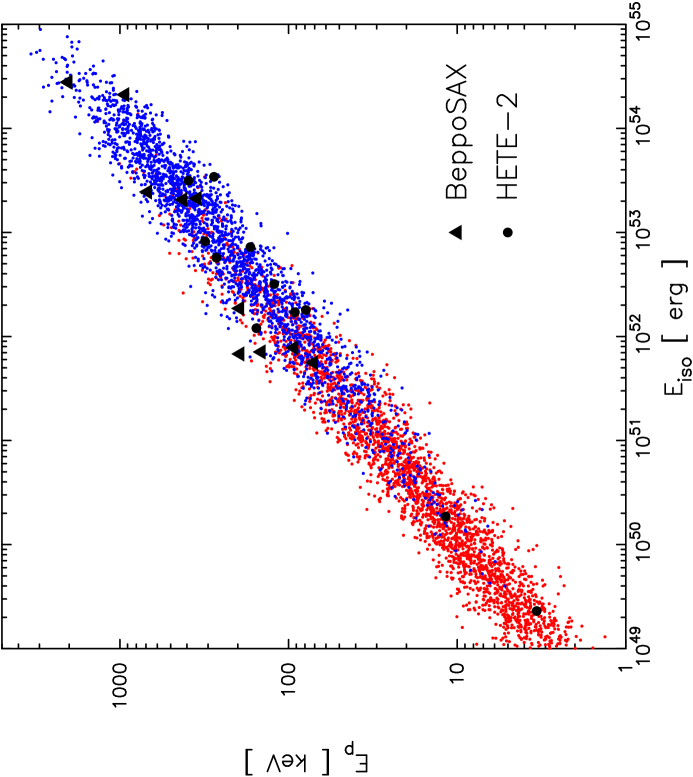
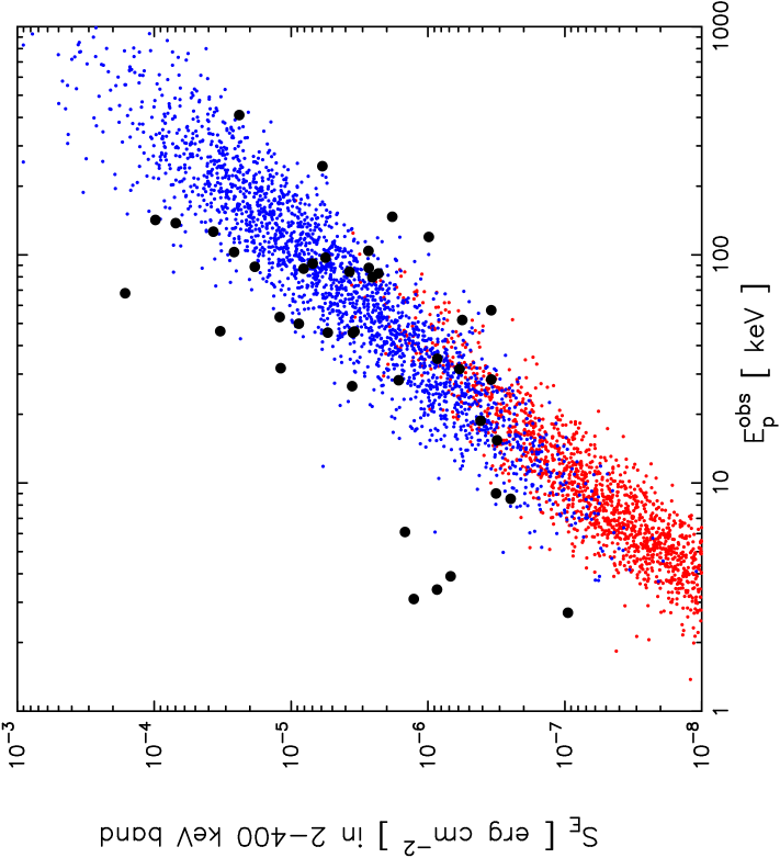
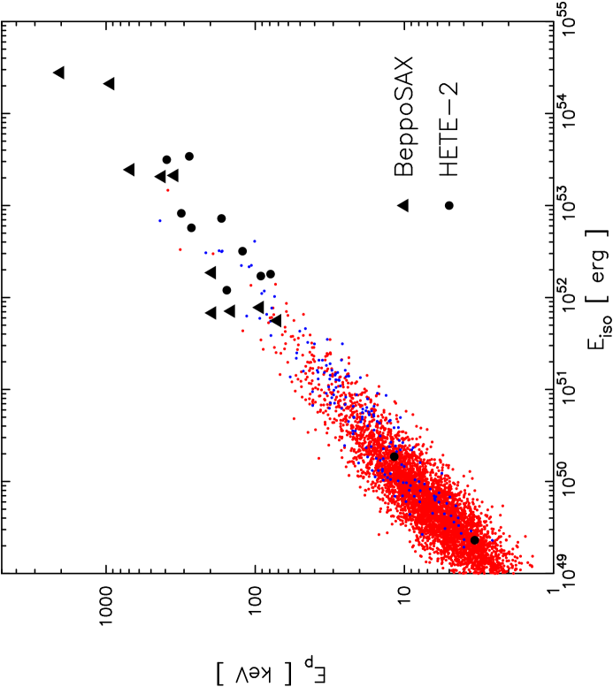
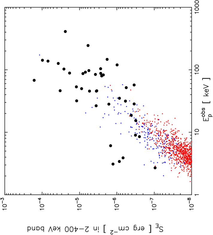
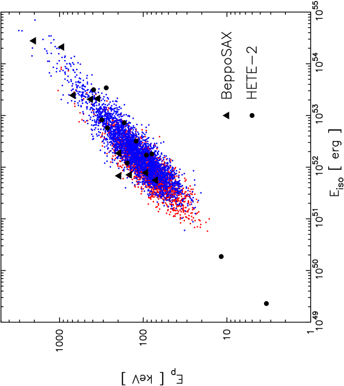
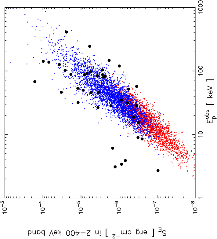
Figure 13: Scatter plots of $E_{\rm iso}$ versus $E_{\rm peak}$ (left column) and $E_{\rm peak}$ versus $S_{E}$ (right column). The top panels show the predicted distributions in the variable jet opening-angle model for $\delta=2$, while the middle and the bottom panels show the power-law universal jet model pinned to the $E_{\rm iso}$ values of XRF 020903 and GRB 980326, respectively (see text). Bursts detected by the WXM are shown in blue and non-detected bursts in red. In the left column, the triangles and circles respectively show the locations of the BeppoSAX and HETE-2 bursts with known redshifts. In the right column, the black circles show the locations of all HETE-2 bursts for which joint fits to WXM and FREGATE spectral data have been carried out (Sakamoto et al., 2004b).

Figure 13 shows scatter plots of $E_{\rm iso}$ versus $E_{\rm peak}$ (left column) and $E_{\rm peak}$ versus $S_{E}$ (right column). The top panels show the predicted distributions in the variable jet opening-angle model for $\delta=2$, while the middle and the bottom panels show the power-law universal jet model pinned to the $E_{\rm iso}$ values of XRF 020903 and GRB 980326, respectively. Detected bursts are shown in blue and non-detected bursts in red. In the left column, the black triangles and circles show the locations of the BeppoSAX and HETE-2 bursts with known redshifts. In the right column, the black cirlces show the locations of HETE-2 bursts for which joint fits to WXM and FREGATE spectral data have been carried out (Sakamoto et al., 2004b). The top panels exhibit the constant density of bursts per logarithmic interval in $E_{\rm iso}$, $E_{\rm peak}$, and $S_{E}$ given by the variable jet opening-angle model for $\delta=2$. The middle and bottom panels show the limited range in $E_{\rm iso}$, $E_{\rm peak}$, and $S_{E}$ of detected bursts in the power-law universal jet model. The middle panels show the preponderance of XRFs relative to GRBs predicted in the power-law universal jet model when it is pinned to the $E_{\rm iso}$ value of XRF 020903; i.e., when one attempts to extend the model to include XRFs and X-ray-rich GRBs, as well as GRBs.

Figure 14 compares the observed and predicted cumulative distributions of $E_{\rm iso}$ and $E_{\rm peak}$ for BeppoSAX and HETE-2 bursts with known redshifts, and the observed and predicted cumulative distributions of $S_{E}$ and $E^{\rm obs}_{\rm peak}$ for all HETE-2 bursts. The solid histograms are the observed cumulative distributions. The solid curves are the cumulative distributions predicted by the variable jet opening-angle model for $\delta=2$. The dotted curves are the cumulative distributions predicted by the power-law universal jet model pinned at the $E_{\rm iso}$ value of XRF 020903; i.e., when one attempts to extend the model to include XRFs and X-ray-rich GRBs, as well as GRBs. The dashed curves are the cumulative distributions predicted by the power-law universal jet model pinned at the $E_{\rm iso}$ value of GRB 980326; i.e., when one fits the model only to GRBs. The cumulative distributions in the present figure correspond to those formed by projecting the observed and predicted distributions in Figure 13 onto the $x$- and $y$-axes of the panels in that figure. The present figure shows that variable jet opening-angle model for $\delta=2$ can explain the observed distributions of burst properties reasonably well, especially given that the sample of XRFs with known redshifts is incomplete due to optical observational selection effects (see Section 6.6.1). It also shows that the power-law universal jet model can explain the observed distributions of GRB properties reasonably well, but cannot do so if asked to explain the properties of XRFs and X-ray-rich GRBs, as well as GRBs.

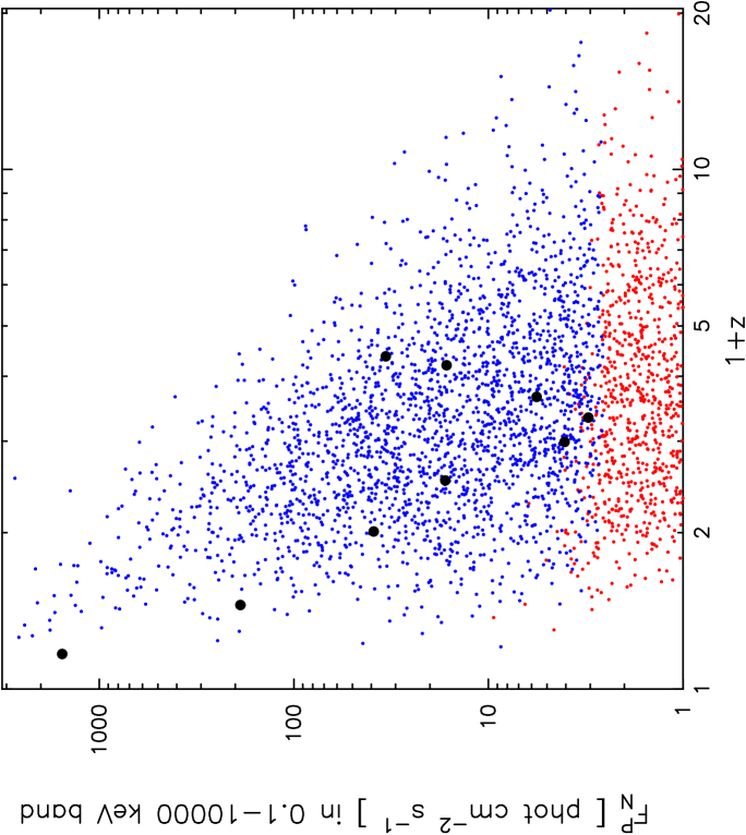
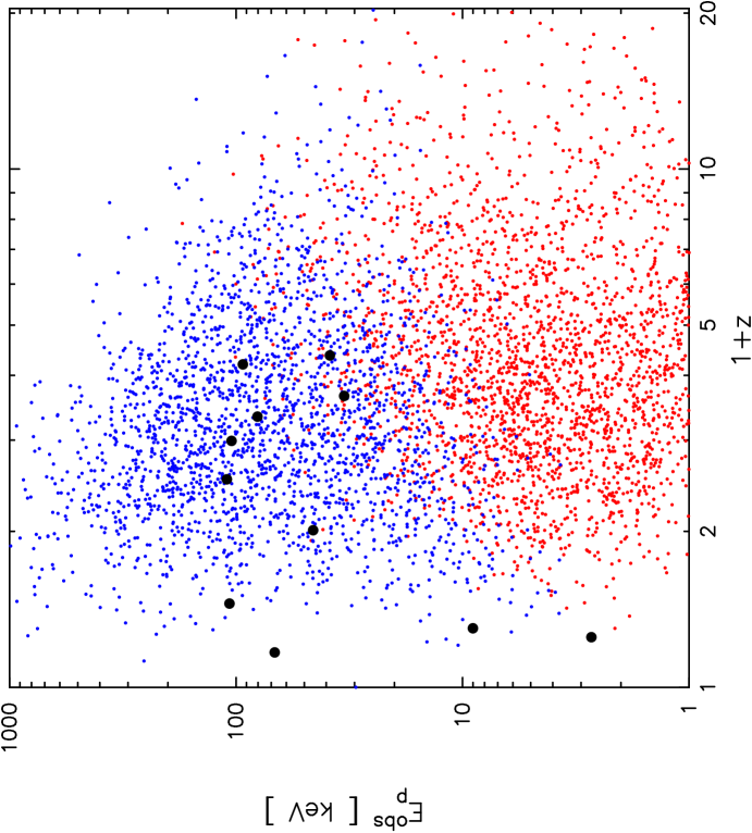
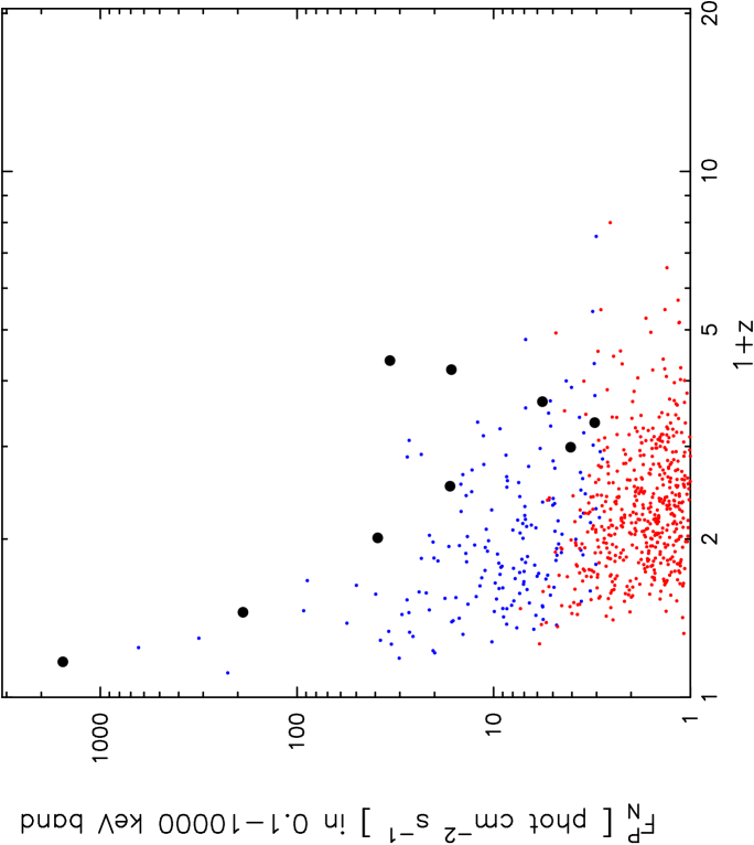
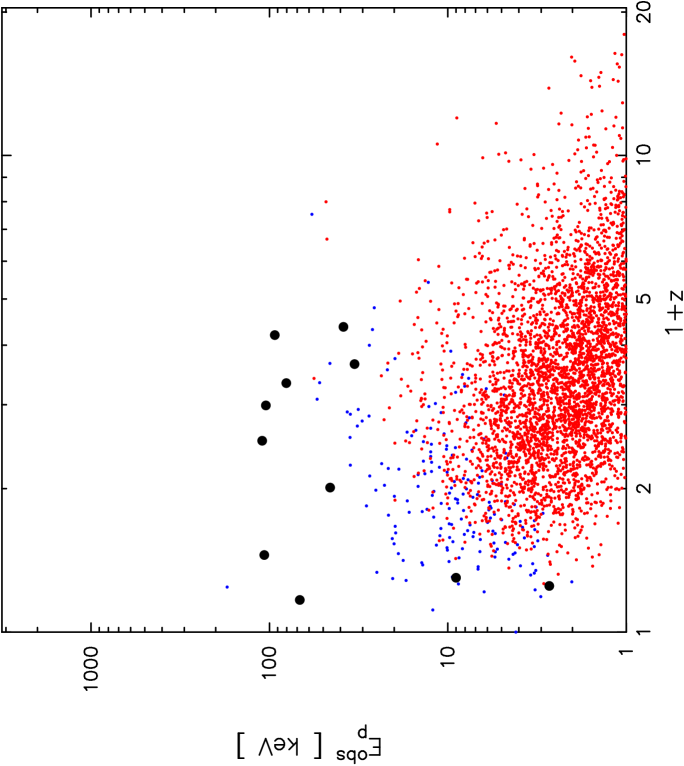
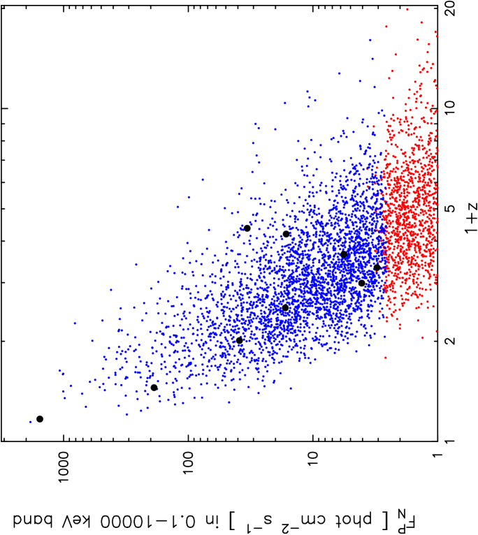
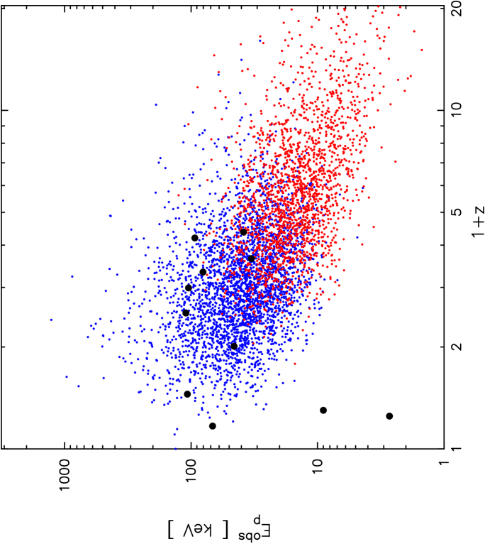
Figure 15: Scatter plots of $F^{\rm P}_{N}$ (left column) and $E^{\rm obs}_{\rm peak}$ (right column) as a function of redshift. The top row shows the distributions of bursts predicted by the variable jet opening-angle model for $\delta=2$. The middle row shows the distributions of bursts predicted by the power-law universal jet model pinned to the $E_{\rm iso}$ value for XRF 020903, while the bottom row shows the distributions of bursts predicted by the power-law universal jet model pinned to the $E_{\rm iso}$ value for GRB 980326. Bursts detected by the WXM are shown in blue and non-detected bursts in red. The filled black circles show the positions of the BeppoSAX and HETE-2 bursts with known redshifts.

Figure 15 shows scatter plots of $F^{\rm P}_{N}$ (left column) and $E^{\rm obs}_{\rm peak}$ (right column) as a function of redshift. The top row shows the distributions of bursts predicted by the variable jet opening-angle model for $\delta=2$. The middle row shows the distributions of bursts predicted by the power-law universal jet model pinned to the $E_{\rm iso}$ value for XRF 020903, while the bottom row shows the distributions of bursts predicted by the power-law universal jet model pinned to the $E_{\rm iso}$ value for GRB 980326. Detected bursts are shown in blue and non-detected bursts in red. The black circles show the positions of the HETE-2 bursts with known redshifts. This figure shows that variable jet opening-angle model for $\delta=2$ can explain the observed distributions of bursts in the ($1+z,F^{\rm P}_{N}$)- and ($1+z,E^{\rm obs}_{\rm peak}$)-planes reasonably well. It also shows that the power-law universal jet model can explain the observed distributions of GRBs alone reasonably well, but cannot explain the observed distributions of XRFs, X-ray-rich GRBs, and GRBs. These conclusions are confirmed by Table 2, which shows the percentages of XRFs, X-ray-rich GRBs, and hard GRBs in the HETE-2 data, and predicted by the variable jet opening-angle model and the power-law universal jet model.

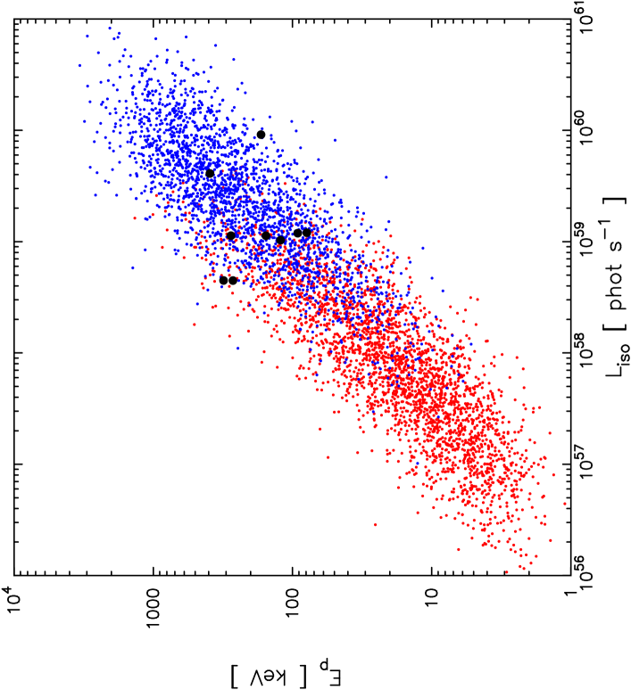
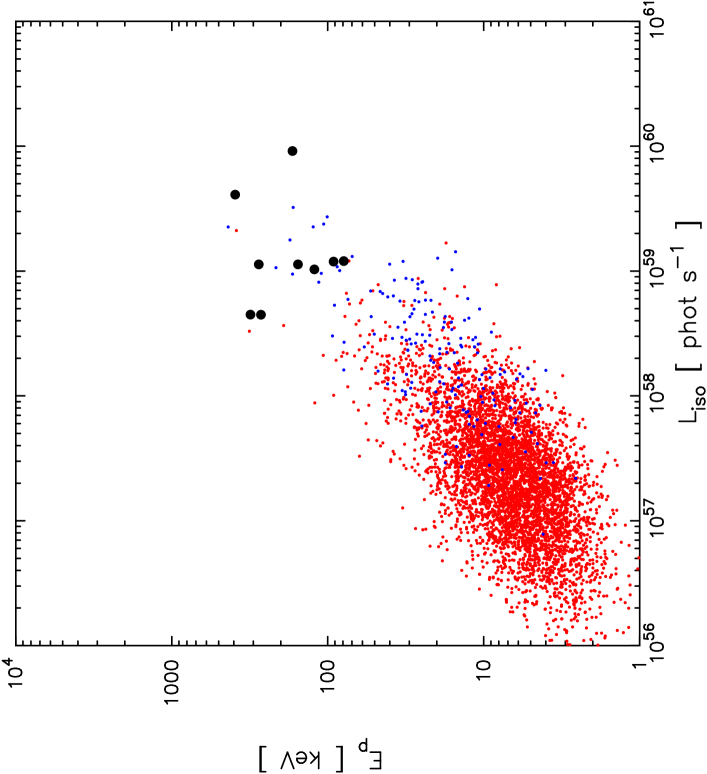
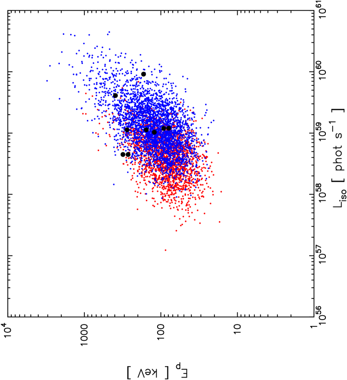
Figure 16: Scatter plots of $L_{\rm iso}$ versus $E_{\rm peak}$ and comparison of observed and predicted cumulative distributions of $L_{\rm iso}$. Upper left: Distribution of bursts predicted by the variable jet opening-angle model for $\delta=2$. Bursts detected by the WXM are shown in blue and non-detected bursts in red. The filled black circles show the positions of the HETE-2 bursts with known redshifts. Upper right: Observed cumulative distribution of $L_{\rm iso}$ for HETE-2 bursts with known redshifts (histogram) compared against the cumulative $L_{\rm iso}$ distributions predicted by the variable jet opening-angle model for $\delta=2$ (solid curve) and by the power-law universal jet model pinned at the $E_{\rm iso}$ value for XRF 020903 (dotted curve) and for GRB 980326 (dashed curve). Lower left: Distribution of bursts predicted by the power-law universal jet model pinned at the $E_{\rm iso}$ value for XRF 020903. Lower right: Distribution of bursts predicted by the power-law universal jet model pinned at the $E_{\rm iso}$ value for GRB 980326.

Figure 16 shows scatter plots of $L_{\rm iso}$ versus $E_{\rm peak}$ and a comparison of the observed and predicted cumulative distributions of $L_{\rm iso}$. The upper left panel shows the distribution of bursts predicted by the variable jet opening-angle model for $\delta=2$. The lower left panel shows the distribution of bursts predicted by the power-law universal jet model pinned at the $E_{\rm iso}$ value for XRF 020903. The lower right panel shows the power-law universal jet model pinned at the $E_{\rm iso}$ value for GRB 980326. Detected bursts are shown in blue and non-detected bursts in red. The black circles show the positions of the HETE-2 bursts with known redshifts. The upper right panel shows the observed cumulative distribution of $L_{\rm iso}$ for HETE-2 bursts with known redshifts (histogram) compared with the cumulative $L_{\rm iso}$ distribution predicted by the variable jet opening-angle model for $\delta=2$ (solid curve), and the cumulative $L_{\rm iso}$ distributions predicted by the power-law universal jet model pinned at the $E_{\rm iso}$ value for XRF 020903 (dotted curve) and for GRB 980326 (dashed curve). The figure shows that the variable jet opening-angle model for $\delta=2$ can explain the observed cumulative distributions of bursts in the ($L_{\rm iso},E_{\rm peak}$)-plane reasonably well. It also shows that the power-law universal jet model can explain the observed distribution of $L_{\rm iso}$ for GRBs alone reasonably well, but cannot explain the observed distribution for XRFs, X-ray-rich GRBs, and GRBs.

The left panel of Figure 17 shows the observed cumulative distribution of $F^{\rm P}_{E}$ for HETE-2 bursts (histogram) compared with the cumulative $F^{\rm P}_{E}$ distribution predicted by the variable jet opening-angle model for $\delta=2$ (solid curve), and the cumulative $F^{\rm P}_{E}$ distributions predicted by the power-law universal jet model pinned at the $E_{\rm iso}$ value for XRF 020903 (dotted curve) and for GRB 980326 (dashed curve). This figure shows that variable jet opening-angle model for $\delta=2$ can explain the observed cumulative distribution of $F^{\rm P}_{E}$ for HETE-2 bursts reasonably well. It also shows that the power-law universal jet model can explain the observed cumulative distribution of $F^{\rm P}_{E}$ for GRBs alone reasonably well, but cannot explain the observed distribution for XRFs, X-ray-rich GRBs, and GRBs seen by HETE-2. All three models have some difficulty explaining the cumulative $F^{\rm P}_{E}$ distribution for BATSE bursts (Donaghy, Graziani & Lamb, 2004b). The right panel of Figure 17 shows the differential distribution of $E^{\rm obs}_{\rm peak}$ predicted by the variable jet opening-angle model for $\delta=2$ for bursts with $F^{\rm P}_{E}>10^{-8}$ (solid histogram), $10^{-7}$ (dashed histogram), and $10^{-6}$ erg cm${-2}$ s^-1 (dotted histogram). The last distribution is in rough agreement with that found by Preece et al. (2000) for BATSE bursts with $F^{\rm P}_{E}\gtrsim 5\times 10^{-7}$ erg cm^-2 s^-1 and $S_{E}>4\times 10^{-5}$ erg cm^-2.

6 Discussion

6.1 Structure of GRB Jets

Motivated by the HETE-2 results, we have explored in this paper the possibility of a unified jet model of XRFs, X-ray-rich GRBs, and GRBs. The HETE-2 results show that $S_{E}$ and $E_{\rm iso}$ decrease by a factor $\sim 10^{5}$ in going from GRBs to XRFs (see Figures 1 and 2). Figures 13 - 16 show that the variable jet opening-angle model can accomodate the large observed ranges in $S_{E}$ and $E_{\rm iso}$ reasonably well, while the power-law universal jet model cannot.

Figures 13-16 show that the variable jet opening-angle model with $\delta=2$ can explain a number of the observed properties of GRBs reasonably well. These figures show that the power-law universal jet model (Rossi, Lazzati & Rees, 2002; Zhang & Mészáros, 2002; Mészáros, Ramirez-Ruiz, Rees & Zhang, 2002; Zhang, Woosley & Heger, 2004; Perna, Sari & Frail, 2003) with $E_{\rm iso}\propto\theta_{\rm view}^{-2}\propto\Omega_{\rm view}^{-1}$ (Zhang & Mészáros, 2002; Rossi, Lazzati & Rees, 2002; Perna, Sari & Frail, 2003) can also explain a number of the observed properties of GRBs reasonably well [see also Rossi, Lazzati & Rees (2002); Perna, Sari & Frail (2003)].

However, as we have seen, HETE-2 has provided strong evidence that the properties of XRFs, X-ray-rich GRBs, and GRBs form a continuum in the ($E_{\rm iso},E_{\rm peak}$)-plane (Lamb et al., 2004) and in the ($S_{E},E^{\rm obs}_{\rm peak}$)-plane (Sakamoto et al., 2004b), and therefore that these three kinds of bursts are the same phenomenon. If this is true, it implies that the $E_{\gamma}$ inferred by Frail et al. (2001), Panaitescu & Kumar (2001) and Bloom, Frail & Kulkarni (2003) is too large by a factor of at least 100. The reason is that the values of $E_{\rm iso}$ for XRF 020903 (Sakamoto et al., 2004a) and XRF 030723 (Lamb et al., 2004) are $\sim$ 100 times smaller than the value of $E_{\gamma}$ inferred by Frail et al. (2001) and Panaitescu & Kumar (2001) – an impossibility.

The reason is that the predictions of the variable jet opening-angle and power-law universal jet models differ dramatically if they are required to accomodate the large observed ranges in $S_{E}$ and $E_{\rm iso}$. Taking $N(\Omega_{\rm jet})\sim\Omega_{\rm jet}^{-2}$ (i.e., $\delta=2$), the variable jet opening-angle model predicts equal numbers of bursts per logarithmic decade in $S_{E}$ and $E_{\rm iso}$, which is exactly what HETE-2 sees (Lamb et al., 2004; Sakamoto et al., 2004b)(see Figures 13 and 14). On the other hand, in the power-law universal jet model the probability of viewing the jet at a viewing angle $\theta_{\rm view}$ is $d\Omega_{\rm view}$, where $\Omega_{\rm view}$ is the solid angle contained within the angular radius $\theta_{\rm view}$. Consequently, most viewing angles $\theta_{\rm view}$ will be $\theta_{\rm view,max}$ or $\approx 90^{\circ}$, whichever is smaller. This implies that the number of XRFs should exceed the number of GRBs by many orders of magnitude, something that HETE-2 does not observe (again, see Figures 13 and 14).

Threshold effects can offset this prediction of the power-law universal jet model over a limited range in $S_{E}$ and $E_{\rm iso}$. This is what enables the power-law universal jet model to explain a number of the observed properties of GRBs reasonably well (Rossi, Lazzati & Rees, 2002; Perna, Sari & Frail, 2003). However, threshold effects cannot offset this prediction over a large range in $S_{E}$ and $E_{\rm iso}$, as our simulations confirm. This is why the power-law universal jet model cannot accomodate the large observed ranges in $S_{E}$ and $E_{\rm iso}$.

We conclude that, if $S_{E}$ and $E_{\rm iso}$ span ranges of $\sim 10^{5}$, as the HETE-2 results strongly suggest, the variable jet opening-angle model can provide a unified picture of XRFs and GRBs, whereas the power-law universal jet model cannot. Thus XRFs may provide a powerful probe of GRB jet structure.

6.2 Rate of GRBs and the Nature of Type Ic Supernovae

A range in $E_{\rm iso}$ of $10^{5}$, which is what the HETE-2 results strongly suggest, requires a minimum range in $\Delta\Omega_{\rm jet}$ of $10^{4}-10^{5}$ in the variable jet opening-angle model. Thus the unified picture of XRFs and GRBs in the variable jet opening-angle model implies that the total number of bursts is

$$N_{\rm total}=-\int^{\Omega_{\rm jet}^{\rm max}}_{\Omega_{\rm jet}^{\rm min}}d\Omega_{\rm jet}\Omega_{\rm jet}^{-2}\approx(\Omega_{\rm jet}^{\rm min})^{-1}\;.$$ (26)

Thus there are $2\pi/\Omega_{\rm jet}^{\rm min}\sim 10^{5}$ more bursts with very small $\Omega_{\rm jet}$’s for every burst that is observable; i.e., the rate of GRBs may be $\sim 100$ times greater than has been thought.

In addition, since the observed ratio of the rate of Type Ic SNe to the rate of GRBs in the observable universe is $R_{\rm Type\ Ic}/R_{\rm GRB}\sim 10^{5}$ (Lamb, 1999, 2000), the variable jet opening-angle model implies that the rate of GRBs could be comparable to the rate of Type Ic SNe. More spherically symmetric jets yield XRFs and narrower jets produce GRBs. Thus low $E_{\rm peak}$ (intrinsically faint) XRFs may probe core collapse supernovae that produce wide jets, while high $E_{\rm peak}$ (intrinsically luminous) GRBs may probe core collapse supernovae that produce very narrow jets (possibly implying that the cores of the progenitor stars of these bursts are rapidly rotating).

Thus XRFs and GRBs may provide a combination of GRB/SN samples that would enable astronomers to study the relationship between the degree of jet-like behavior of the GRB and the properties of the supernova (brightness, polarization $\Leftrightarrow$ asphericity of the explosion, velocity of the explosion $\Leftrightarrow$ kinetic energy of the explosion, etc.). GRBs may therefore provide a unique laboratory for understanding Type Ic core collapse supernovae.

6.3 Constraints on $\Omega_{\rm jet}^{\rm min}$ and $\Omega_{\rm jet}^{\rm max}$

The HETE-2 results require a range in $\Omega_{\rm jet}$ of $\sim 10^{5}$ within the context of the variable jet opening-angle model in order to explain the observed ranges in $S_{E}$ and $E_{\rm iso}$. Thus the HETE-2 results fix the ratio $\Omega_{\rm jet}^{\rm max}/\Omega_{\rm jet}^{\rm min}$, but not $\Omega_{\rm jet}^{\rm min}$ and $\Omega_{\rm jet}^{\rm max}$ separately. However, geometry and observations strongly constrain the possible values of $\Omega_{\rm jet}^{\rm min}$ and $\Omega_{\rm jet}^{\rm max}$. In this paper, we have adopted $\Omega_{\rm jet}^{\rm max}=0.6\times 2\pi\ {\rm sr}$ (i.e., $\theta_{\rm jet}=70^{\circ}$), which is nearly the maximum value allowed by geometry. However, it seems physically unlikely that GRB jets can have jet opening angles as large as $\approx 90^{\circ}$. One might therefore wish to adopt a smaller value of $\Omega_{\rm jet}^{\rm max}$. This would imply a smaller value of $\Omega_{\rm jet}^{\rm min}$ and therefore a larger GRB rate. But the GRB rate cannot be larger than the rate of Type Ic SNe. Therefore $\Omega_{\rm jet}^{\rm min}$ cannot be much smaller than the value $\Omega_{\rm jet}^{\rm min}=0.6\times 2\pi\times 10^{-5}\ {\rm sr}=3.8\times 10^{-5}\ {\rm sr}$ that we have adopted.

Even the value $\Omega_{\rm jet}^{\rm min}=3\times 10^{-5}\ {\rm sr}$ implies GRB jet opening solid angles that are a factor of $\approx$ 100 smaller than those inferred from jet break times by Frail et al. (2001), Panaitescu & Kumar (2001) and Bloom, Frail & Kulkarni (2003). There is a substantial uncertainty in the jet opening solid angle implied by a given jet break time, but the uncertainty is thought to be a factor of $\sim 20$, not a factor $\sim 100$ (Rhoads, 1999; Sari, Piran & Halpern, 1999). In addition, the global modeling of GRB afterglows is largely free from this uncertainty. Such modeling tends to find jet opening angles $\theta_{\rm jet}$ of a few degrees for the brightest and hardest GRBs (Panaitescu & Kumar, 2001, 2003) – values of $\theta_{\rm jet}$ that are a factor of at least 3, and in some cases a factor of 10, larger than the jet opening angles we use in this work. This is discomforting; adopting a still smaller value of $\Omega_{\rm jet}^{\rm min}$ would be even more discomforting.

Another constraint on $\Omega_{\rm jet}^{\rm min}$ comes from the monitoring of the late-time radio emission of a sample of 33 nearby Type Ic SNe that has been carried out by Berger et al. (2003c). They find that the energy emitted at radio wavelengths by this sample of Type Ic SNe is $E_{\rm radio}<10^{48}$ ergs in almost all cases. This implies that these supernovae do not produce jets with energies $E_{\rm jet}>10^{48}$ ergs, and therefore that at most $\sim$ 4% of all nearby Type Ic SNe produce GRBs, assuming $E_{\gamma}=1.4\times 10^{51}$ ergs. In the variable jet opening-angle model, $E_{\gamma}$ is a factor $\approx$ 100 times less than this value, which weakens the constraint on the allowed fraction of Type Ic SNe that produce GRBs to $\lesssim$ 10%. Adopting a still smaller value of $\Omega_{\rm jet}^{\rm min}$ would decrease $E_{\gamma}$ and therefore increase the allowed fraction of Type Ic SNe that produce GRBs. However, a smaller value of $\Omega_{\rm jet}^{\rm min}$ would also increase the predicted numbers (and therefore the fraction) of Type Ic SNe that produce GRBs. Thus, while not yet contradicting the variable jet opening-angle model of XRFs and GRBs, the radio monitoring of nearby Type Ic SNe carried out by Berger et al. (2003c) places an important constraint on $\Omega_{\rm jet}^{\rm min}$.

In Section 6.6.1, we report tantalizing evidence that the efficiency with which the kinetic energy in the jet is converted into prompt emission at X-ray and $\gamma$-ray wavelengths may decrease as $E_{\rm iso}$ and $E_{\rm peak}$ decreases; i.e., this efficiency may be less for XRFs than for GRBs [see also Lloyd-Ronning & Zhang (2004)]. Since $E_{\rm iso}$ spans five decades in going from XRFs to GRBs, even a modest rate of decline in this efficiency with $E_{\rm iso}$ would reduce the required range in $\Delta\Omega_{\rm jet}$ by a factor of ten or more. Such a factor would allow $\Omega_{\rm jet}^{\rm min}$ to be increased to $\Omega_{\rm jet}^{\rm min}\approx 4\times 10^{-4}$ sr or more, which would bring the jet opening-angle for GRBs in the variable jet opening angle model into approximate agreement with the values derived from global modeling of GRB afterglows. It would also reduce the predicted rate of GRBs by a factor of ten or more, and therefore also reduce the fraction of Type Ic SNe that produce GRBs to $\sim$ 10% or less, in agreement with the constraint derived from radio monitoring of nearby Type Ic SNe. We note that including such a decrease of efficiency with $E_{\rm iso}$ and $E_{\rm peak}$ would introduce an additional parameter into the model.

6.4 Outliers

Bloom, Frail & Kulkarni (2003) and Berger et al. (2003b) have called attention to the fact that not all GRBs have values of $E_{\gamma}$ that lie within a factor of 2-3 of the standard energy $E_{\gamma}$; i.e., that there are outliers in the $E_{\gamma}$ distribution. Berger et al. (2003c) have also proposed a core/halo model for the jet in GRB 030329.

In addition, we note that the two XRFs for which redshifts or strong redshifts constraints exist (the HETE–localized bursts XRF 020903 and XRF 030723) lie squarely on the relation between $E_{\rm iso}$ and $E_{\rm peak}$ found by Amati et al. (2002) (see Figure 2). The implied value of $E_{\gamma}$ from the absence of a jet break in the optical afterglow of XRF 020903 is $\approx 1.1\times 10^{49}$ ergs (Soderberg et al., 2003), which is consistent with the standard energy of $E_{\gamma}=1.17\times 10^{49}$ ergs that we use in this work. However, the implied value of $E_{\gamma}$ from the jet break time of $\sim$ 1 day in XRF 030723 (Dullighan et al., 2003) is a factor $\sim 100$ smaller than the standard energy that we use in this work and a factor $\sim 10^{4}$ smaller than the standard energy of $E_{\gamma}=1.3\times 10^{51}$ found by Bloom, Frail & Kulkarni (2003) [see also Frail et al. (2001) and Panaitescu & Kumar (2001)].

The unified jet model of XRFs, X-ray-rich GRBs, and GRBs that we have proposed is a phenomenological one, and is surely missing important aspects of the GRB jet phenomenon, which may include a significant stochastic element. It therefore cannot be expected to account for the properties of all bursts. Only further observations can say whether the bursts discussed above (or others) are a signal that the unified jet model is missing important aspects of GRB jets, or whether they are truly outliers.

6.5 Variable Jet Opening-Angle Model in the MHD Jet Picture

Zhang & Mészáros (2003) and Kumar & Panaitescu (2003) have studied the early afterglows of two GRBs. Zhang & Mészáros (2003) find in the case of GRB 990123 strong evidence that the jet is magnetic energy dominated; Kumar & Panaitescu (2003) reach a similar conclusion for GRB 021211. In both cases, it appears that the magnetic energy dominated the kinetic energy in the ejected matter by a factor $>$ 1000. The recent discovery that the prompt emission from GRB 021206 was strongly polarized (Coburn & Boggs, 2003) may provide further support for the picture that GRBs come from magnetic-energy dominated jets.

Part of the motivation for the power-law universal jet model comes from the expectation that in hydrodynamic jets, entrainment and the interaction of the ultra-relativistic outflow with the core of the progenitor star may well result in a strong fall-off of the velocity of the flow away from the jet axis. Thus the narrow jets we find in the unified picture of XRFs, X-ray-rich GRBs and GRBs based on the variable jet opening-angle model are difficult to reconcile with hydrodynamic jets. They may be much easier to understand if GRB jets are magnetic-energy dominated; i.e., if GRBs come from MHD jets. Such jets can be quite narrow (Vlahakis & Königl, 2001; Proga et al., 2003; Fendt & Ouyed, 2003) and may resist the entrainment of material from the core of the progenitor star.

6.6 Possible Tests of the Variable Jet Opening-Angle Model

6.6.1 X-Ray and Gamma-Ray Observations

We have shown that a unified picture of XRFs and GRBs based on the variable jet opening-angle model has profound implications for the structure of GRB jets, the rate of GRBs, and the nature of Type Ic supernovae. Obtaining the evidence needed to confirm (or possibly rule out) the variable jet opening-angle model and its implications will require the determination of both the spectral parameters and the redshifts of many more XRFs. The broad energy range of HETE-2 (2-400 keV) means that it is able to accurately determine the spectral parameters of the XRFs that it localizes. This will be more difficult for Swift, whose spectral coverage (15-150 keV) is more limited.

Until very recently, only one XRF (XRF 020903; Soderberg et al. 2003) had a probable optical afterglow and redshift (see Figure 18). This is because the X-ray (and by implication the optical) afterglows of XRFs are $\sim 10^{3}$ times fainter than those of GRBs (see Figure 19; see also Lamb et al. (2005) [in preparation]). However, we find that the best-fit slope of the correlation between $L_{\rm X,iso}$ and $L_{\rm iso}$ is not $+1$, but $+0.74\pm 0.17$. This implies that the fraction of the kinetic energy of the jet that goes into the burst itself decreases as $L_{\rm iso}$ (and therefore $E_{\rm iso}$) decreases; i.e., the fraction of the kinetic energy in the jet that goes into the X-ray and optical afterglow is much larger for XRFs than it is for GRBs.

This result is consistent with a picture in which the central engines of XRFs produce less variability in the outflow of the jet than do the central engines of GRBs, resulting in less efficient extraction of the kinetic energy of the jet in the burst itself in the case of XRFs than in the case of GRBs. Such a picture is supported by studies that suggest that the temporal variability of a burst is a good indicator of the isotropic-equivalent luminosity $L_{\rm iso}$ of the burst (Fenimore & Ramirez-Ruiz, 2000; Reichart et al., 2001a). These studies imply that XRFs, which are much less luminous than GRBs, should exhibit much less temporal variability than GRBs. As we discussed in Section 6.3, if the efficiency with which the kinetic energy in the jet is converted into prompt emission at X-ray and $\gamma$-ray wavelengths decreases even modestly with decreasing $E_{\rm iso}$, it would reduce the required range in $\Delta\Omega_{\rm jet}$ by a factor of ten or more, allowing the opening angle for GRBs in the variable jet opening-angle model to be brought into approximate with the values derived from global modeling of GRB afterglows (Panaitescu & Kumar, 2001, 2003) and the rate of GRBs to be brought into agreement with the constraint derived from radio monitoring of nearby Type Ic SNe (Berger et al., 2003c).

The above picture differs from the core-halo picture of GRB jets recently proposed by Berger et al. (2003b), in which the prompt burst emission and the early X-ray and optical afterglows are due to a narrow jet, while the later optical and the radio afterglows are due to a broad jet. In this picture, the total kinetic energy $E_{\rm jet}$ of the jet is roughly constant, but the fraction of $E_{\rm jet}$ that is radiated in the narrow and the broad components can vary.

The challenge presented by the fact that the X-ray (and by implication the optical) afterglows of XRFs are $\sim 10^{3}$ times fainter than those of GRBs can be met: the recent HETE-2–localization of XRF 030723 represents the first time that an XRF has been localized in real time (Prigozhin et al., 2003); identification of its X-ray (Butler et al. 2003a,b) and optical (Fox et al., 2003) afterglows rapidly followed. This suggests that Swift’s ability to rapidly follow up GRBs with the XRT and UVOT – its revolutionary feature – will greatly increase the fraction of bursts with known redshifts.

A partnership between HETE-2 and Swift, in which HETE-2 provides the spectral parameters for XRFs, and Swift slews to the HETE-2–localized XRFs and provides the redshifts, can provide the data that is required in order to confirm (or possibly rule out) the variable jet opening-angle model and its implications. This constitutes a compelling scientific case for continuing HETE-2 during the Swift mission.

6.6.2 Global Modeling of GRB Afterglows

Panaitescu & Kumar (2003) have modeled in detail the afterglows of GRBs 990510 and 000301c. In both cases, they find that fits to the X-ray, optical, NIR, and radio data for GRBs 990510 and 000301c favor the variable jet opening-angle model over the power-law universal jet model. Detailed modeling of the afterglows of other GRBs may provide further evidence favoring one phenomenological jet model over the other for particular bursts.

6.6.3 Polarization of GRBs and Their Afterglows

The variable jet opening-angle model and the power-law universal jet model predict different behaviors for the polarization of the optical afterglow. The variable jet opening-angle model predicts that the polarization angle should change by $180^{\circ}$ over time, passing through $0$ around the time of the jet break in the afterglow light curve. In contrast, the power-law universal jet model predicts that the polarization angle should not change with time. The polarization data on GRB afterglows that has been obtained to date is in most cases very sparse, making it difficult to tell whether or not the behavior of the polarization favors the variable jet opening-angle or the power-law universal jet model.

In the case of GRB 021004, however, the data shows clear evidence that the polarization angle changed by approximately $180^{\circ}$ and changed sign at roughly the time of the jet break, as the variable jet opening-angle model, but not the power-law universal jet model, predicts (Rol et al., 2003). Thus, in the case of this one GRB, at least, the behavior of the polarization of the optical afterlow favors the variable jet opening-angle model over the power-law universal jet model.

6.7 Rate of Detection of GRBs by Gravitational Wave Detectors

If, as the variable jet opening-angle model of XRFs, X-ray-rich GRBs and GRBs implies, most GRBs are bright and have narrow jets – possibly implying that the collapsing core of the progenitor star may be rapidly rotating – GRBs might be detectable sources of gravitational waves. If as has been argued, $E_{\rm gw}/E_{\rm rot}\sim$ 5% in the formation of a black hole from the collapse of the core of the Type Ic supernova (van Putten & Levinson, 2002), where $E_{\rm gw}$ is the energy emitted in gravitational waves and $E_{\rm rot}$ is the rotational energy of the newly formed black hole, and the rate of GRBs is $\sim$ 100 times higher than has been thought, then the rate of LIGO/VIRGO detections of GRBs might be $\sim$ 5 yr^-1 rather than $\sim$ 1 yr^-1 (van Putten & Levinson, 2002).

7 Conclusions

In this paper we have shown that a variable jet opening-angle model, in which the isotropic-equivalent energy $E_{\rm iso}$ depends on the jet solid opening angle $\Omega_{\rm jet}$, can account for many of the observed properties of XRFs, X-ray-rich GRBs, and GRBs in a unified way. We have also shown that, although the power-law universal jet model can account reasonably well for many of the observed properties of GRBs, it cannot easily be extended to accommodate XRFs and X-ray-rich GRBs. The variable jet opening-angle model implies that the total radiated energy in gamma rays $E_{\gamma}$ is $\sim 100$ times smaller than has been thought. The model also implies that the hardest and most brilliant GRBs have jet solid angles $\Omega_{\rm jet}/2\pi\sim 10^{-5}$. Such small solid angles are difficult to achieve with hydrodynamic jets, and lend support to the idea that GRB jets are magnetic-energy dominated. Finally, the variable jet opening-angle model implies that there are $\sim 10^{5}$ more bursts with very small $\Omega_{\rm jet}$’s for every observable burst. The observed ratio of the rate of Type Ic SNe to the rate of GRBs is $R_{\rm TypeIc}/R_{\rm GRB}\sim 10^{5}$; the variable jet opening-angle model therefore implies that the GRB rate may be comparable to the rate of Type Ic SNe, with more spherically symmetric jets yielding XRFs and narrower jets producing GRBs. GRBs may therefore provide a unique laboratory for understanding Type Ic core collapse supernovae.

Table 1: Parameters of Lognormal Distributions

Quantity	Central Value	Sigma	Source of Data
Energy Radiated: Log $E_{\gamma}$[erg]	$51.070\pm 0.095$	$0.33^{+0.08}_{-0.06}$	1
$E_{\rm iso}$-$E_{\rm peak}$ Relation: Log $C$[kev]	$1.950\pm 0.040$	$0.13$	2, 3
Conversion Timescale: Log $T$ [sec]	$0.574\pm 0.075$	$0.305^{+0.062}_{-0.049}$	2, 3

Table 2: Percentages of XRFs, X-Ray-Rich GRBs, and Hard GRBs in HETE-2 Data and Predicted by Different Jet Models

HETE-2 Data or Model	XRFs (%)	X-Ray-Rich GRBs (%)	Hard GRBs (%)
HETE-2 Data	$33$	$44$	$22$
Variable Opening-Angle Jet	$22$	$39$	$39$
PL Universal Jet pinned to 020903	$89$	$10$	$1.0$
PL Universal Jet pinned to 980326	$32$	$56$	$12$

Figure 1: Distribution of HETE-2 bursts in the [$S(2-400{\rm keV}),E^{\rm obs}_{\rm peak}$]-plane, showing XRFs (filled circles), X-ray-rich GRBs (open boxes), and GRBs (filled boxes). This figure shows that XRFs and X-ray-rich GRBs comprise about 2/3 of the bursts observed by HETE-2 , and that the properties of the three kinds of bursts form a continuum. All error bars are 90% confidence level. From Sakamoto et al. (2004b).

Figure 2: Left panel: distribution of HETE-2 and BeppoSAX bursts in the ($E_{\rm iso}$,$L_{\rm iso}$)-plane, where $E_{\rm iso}$ and $L_{\rm iso}$ are the isotropic-equivalent GRB energy and luminosity in the source frame. Middle panel: distribution of HETE-2 and BeppoSAX bursts in the ($E_{\rm iso}$,$E_{\rm peak}$)-plane, where $E_{\rm peak}$ is the energy of the peak of the burst $\nu F_{\nu}$ spectrum in the source frame. The HETE-2 bursts confirm the relation between $E_{\rm iso}$ and $E_{\rm peak}$ found by Amati et al. (2002) and extend it by a factor $\sim 300$ in $E_{\rm iso}$. Right panel: distribution of HETE-2 and BeppoSAX bursts in the ($L_{\rm iso}$,$E_{\rm peak}$)-plane. The distribution of HETE-2 and BeppoSAX bursts in the three planes demonstrates that there is a linear relation between $\log E_{\rm iso}$ and $\log L_{\rm iso}$ that extends over at least five decades in both quantities, and are linear relations between both $\log E_{\rm iso}$ and $\log L_{\rm iso}$ and $\log E_{\rm peak}$ that extend over at least 2.5 decades in $E_{\rm peak}$. The bursts with the lowest and second-lowest values of $E_{\rm iso}$ and $L_{\rm iso}$ are XRFs 020903 and 030723. From Lamb et al. (2004); BeppoSAX data is from Amati et al. (2002).

Figure 4: Left panel: distribution of HETE-2 and BeppoSAX bursts in the ($2\pi/\Omega_{\rm jet}$,$E_{\rm iso}$)-plane, where $E_{\rm iso}$ is the isotropic-equivalent burst energy in the source frame. In the variable jet opening-angle model, $\Omega_{\rm jet}$ is the jet solid angle; in the power-law universal jet model it is the solid angle interior to the viewing angle $\theta_{\rm view}$. Middle panel: distribution of HETE-2 and BeppoSAX bursts in the ($2\pi/\Omega_{\rm jet}$,$L_{\rm iso}$)-plane, where $L_{\rm iso}$ is the isotropic-equivalent burst luminosity in the source frame. Right panel: distribution of HETE-2 and BeppoSAX bursts in the ($2\pi/\Omega_{\rm jet}$,$E_{\rm peak}$)-plane, where $E_{\rm peak}$ is the energy of the peak of the burst $\nu F_{\nu}$ spectrum in the source frame. The distribution of HETE-2 and BeppoSAX bursts in these three planes demonstrates that there are linear relations between both $\log E_{\rm iso}$ and $\log L_{\rm iso}$ and $\log\Omega_{\rm jet}^{-1}$ that extends over at least 2.5 decades in $\log E_{\rm iso}$ and $\log L_{\rm iso}$, and a relation of slope 1/2 between $\log E_{\rm peak}$ and $\log\Omega_{\rm jet}^{-1}$ that extends over at least a decade in $E_{\rm peak}$. The event in the lower-left corner is XRF 020903, which is shown as a lower-limit in $2\pi/\Omega_{\rm jet}$. Data on $\Omega_{\rm jet}$ is from Bloom, Frail & Kulkarni (2003).

Figure 6: Flowchart showing the logical sequence of the simulations for the variable jet opening-angle model.

Figure 7: Left panels: comparison of the best-fit smearing functions $G(E_{\gamma}$), $G(C)$, and $G(T)$ and the cumulative distributions of $E_{\gamma}$ (top), $\Delta E_{\rm peak}$ (middle), and $T_{0}$ (bottom), respectively. Right panels: $E_{\gamma}$ (top), the deviation $\Delta E_{\rm peak}$ in $E_{\rm peak}$ of bursts from the $E_{\rm iso}-E_{\rm peak}$ relation that we have adopted (middle), and $T_{0}\sim F^{\rm P}_{N}/S_{E}$ (bottom), as a function of redshift $z$. The smaller error bar represents the statistical error, while the larger represents the total error. Closed circles denote HETE-2 points, while open circles denote BeppoSAX points. For more information see the text and Table 1.

Figure 8: GRB rate as a function of redshift that we assume in this paper. The curve is the Rowan-Robinson (2001) function for the star-formation rate [equation (3)], taking $P=1.2$ and $Q=5.4$.

Figure 12: Observed and predicted cumulative distributions of $\Omega_{\rm jet}$. Left panel: Cumulative distributions of $\Omega_{\rm jet}$ predicted by the variable jet opening-angle model for $\delta=1$, $2$ and $3$ (curves from right to left), compared to the observed cumulative distribution of the values of $\Omega_{\rm jet}$ given in Bloom, Frail & Kulkarni (2003) scaled downward by a factor of $C_{\rm jet}$ = 95 (solid histogram). Right panel: Cumulative $\Omega_{\rm jet}\equiv\Omega_{\rm view}$ distributions predicted by the power-law universal jet model with the minimum value of $E_{\rm iso}$ pinned to the value of $E_{\rm iso}$ for XRF 020903 (solid curve) and to the value of $E_{\rm iso}$ for GRB 980326 (dashed curve). Models are compared with observed cumulative distribution of the values of $\Omega_{\rm jet}$ given in Bloom, Frail & Kulkarni (2003) (dashed histogram) and the same scaled downward by a factor of $C_{\rm jet}$ = 95 (solid histogram). See the text for more details.

Figure 14: Comparison of the observed and predicted cumulative distributions of $E_{\rm iso}$ (upper row) and $E_{\rm peak}$ (middle row) for HETE-2 and BeppoSAX bursts with known redshifts; and $S_{E}$ and $E^{\rm obs}_{\rm peak}$ for all HETE-2 bursts (lower row). The solid histograms are the observed cumulative distributions. The blue curves are the cumulative distributions predicted by the variable jet opening-angle model for $\delta=2$. The solid red curves are the cumulative distributions predicted by the power-law universal jet model pinned at the $E_{\rm iso}$ value of XRF 020903; i.e., when one attempts to extend the model to include XRFs and X-ray-rich GRBs, as well as GRBs. The dashed red curves are the cumulative distributions predicted by the power-law universal jet model pinned at the $E_{\rm iso}$ value of GRB 980326; i.e., when one fits the model only to GRBs.

Figure 17: Left panel: Comparison of the observed cumulative distribution of $F^{\rm P}_{E}$ for HETE-2 bursts (histogram) with the cumulative $F^{\rm P}_{E}$ distributions predicted by the variable jet opening-angle model for $\delta=2$ (solid curve) and by the power-law universal jet model pinned at the $E_{\rm iso}$ value for XRF 020903 (dotted curve) and at the $E_{\rm iso}$ value for GRB 980326 (dashed curve). Right panel: Differential distribution of $E^{\rm obs}_{\rm peak}$ predicted by the variable jet opening-angle model for $\delta=2$ for bursts with $F^{\rm P}_{E}>10^{-8}$ (solid histogram), $10^{-7}$ (dashed histogram), and $10^{-6}$ erg cm^-2 s^-1 (dotted histogram).

Figure 18: Distribution of HETE-2 bursts in the [$S(2-400{\rm keV}),E^{\rm obs}_{\rm peak}$]-plane, showing the bursts with redshift determinations (solid squares) and those without (open squares). The two events with known redshifts in the lower left-hand corner of the figure are XRF 020903 and XRF 030723. From Sakamoto et al. (2004b).

Figure 19: Left panel: Correlation between the isotropic-equivalent burst energy ($E_{\rm iso}$) and the X-ray afterglow luminosity ($L_{\rm X,iso}$) at 10 hours after the burst from Berger et al. (2003a). The slope of the best-fit line is $0.74\pm 0.17$ (68% confidence level). Middle panel: Correlation between the X-ray afterglow flux at 10 hours after the burst ($F_{\rm x,10}$) and the peak energy flux ($F^{\rm P}_{E}$). The slope of the best-fit line is $0.35\pm 0.14$ (68% confidence level). Right panel: The ratio $f=F_{\rm x,10}/F^{\rm P}_{E}$ as a function of $F^{\rm P}_{E}$. The slope of the best-fit line is $-0.70\pm 0.15$ (68% confidence level). After Lamb et al. (2005, in preparation).

References

- Amati et al. (2002) Amati, L., et al. 2002, A&A, 390, 81
- Atteia et al. (2003) Atteia, J-L, et al. 2003, in AIP Conf. Proc. 662, Gamma-Ray Burst and Afterglow Astronomy 2001, ed. G. R. Ricker & R. K. Vanderspek (New York: AIP), 17
- Band, et al. (1993) Band, D. L., et al. 1993, ApJ, 413, 281
- Band (2003) Band, D. L. 2003, ApJ, 588, 945
- Barraud et al. (2003) Barraud, C., et al. 2003, A&A, 400, 1021
- Berger et al. (2003a) Berger, E., Kulkarni, S. R., Frail, D. A., & Soderberg, A. M. 2003a, ApJ, 590, 379
- Berger et al. (2003b) Berger, E., et al. 2003b, Nature, 426, 154
- Berger et al. (2003c) Berger, E., et al. 2003c, ApJ, 599, 408