Mass Transfer between Double White Dwarfs

Abstract

Three periodically variable stars have recently been discovered (V407 Vul, $P=9.5\,\min$; ES Cet, $P=10.3\,\min$; RX J0806.3+1527, $P=5.3\,\min$) with properties that suggest that their photometric periods are also their orbital periods, making them the most compact binary stars known. If true, this might indicate that close, detached, double white dwarfs are able to survive the onset of mass transfer caused by gravitational wave radiation and emerge as the semi-detached, hydrogen-deficient stars known as the AM CVn stars. The accreting white dwarfs in such systems are large compared to the orbital separations. This has two effects: first it makes it likely that the mass transfer stream can hit the accretor directly, and second it causes a loss of angular momentum from the orbit which can destabilise the mass transfer unless the angular momentum lost to the accretor can be transferred back to the orbit. The effect of the destabilisation is to reduce the number of systems which survive mass transfer by as much as one hundred-fold. In this paper we analyse this destabilisation and the stabilising effect of a dissipative torque between the accretor and the binary orbit. We obtain analytic criteria for the stability of both disc-fed and direct impact accretion, and carry out numerical integrations to assess the importance of secondary effects, the chief one being that otherwise stable systems can exceed the Eddington accretion rate. We show that to have any effect upon survival rates, the synchronising torque must act on a timescale of order 1000 years or less. If synchronisation torques are this strong, then they will play a significant role in the spin rates of white dwarfs in cataclysmic variable stars as well.

1 Introduction

In recent years there have been discoveries of close detached double white dwarfs at a rate that suggests that there may be of order 200 million such systems in our Galaxy, making them the largest population of close binary stars (e.g. Marsh, Dhillon & Duck 1995; Napiwotzki et al. 2003). These systems were predicted theoretically long ago (Webbink 1979; Webbink 1984; Iben & Tutukov 1984), and were proposed as potential Type Ia supernova progenitors, the explosion being triggered by the action of gravitational wave losses which cause them to merge. Only those systems with total mass in excess of $1.4\,\mathrm{M}_{\odot}$ have the potential to become Type Ia supernovae. These represent only a few percent of merging systems (Iben, Tutukov & Yungelson 1997), which raises the question as to the fate of the less massive systems. Possible outcomes which have been suggested are sdB stars and R CrB stars (Webbink 1984; Iben 1990; Saio & Jeffery 2002). Another possibility is that the stars survive as binary systems to become the semi-detached accreting binary stars known as the AM CVn stars (Nather, Robinson & Stover 1981; Tutukov & Yungelson 1996; Nelemans et al. 2001). These remarkable systems have extremely short orbital periods (17 to 65 minutes) made possible because of the high densities of their degenerate donor stars. Moreover they feature accretion discs composed largely of helium which offer the opportunity to see the effect of abundance upon disc physics.

In their study of the evolution of AM CVn systems, Nelemans et al. (2001) considered the evolution of detached double white dwarfs into the semi-detached phase, which requires the systems to pass through an ultra-compact phase when orbital periods as low as two or three minutes are possible. The stability of the mass transfer during this stage is crucial as to whether the systems survive intact or merge. An additional complication is that even in stable systems the equilibrium mass transfer rate can be (highly) super-Eddington, resulting in mass and angular momentum loss and probably merging of the system (Han & Webbink 1999; Nelemans et al. 2001). Mass transfer between two white dwarfs has generally been taken to be stable if the mass ratio $q=M_{2}/M_{1}$, where $M_{1}$ is the mass of the accretor, is smaller than about $2/3$. However, Nelemans et al. identified the interesting possibility of the mass transfer stream hitting the accreting white dwarf directly during this phase. They realised that mass transfer without an accretion disc may destabilise the mass transfer process for lower mass ratios still because the normal transfer of angular momentum from disc to orbit would be absent.

Assuming that unstable systems do not survive, Nelemans et al. (2001) found that the destabilisation by direct impact accretion could have a dramatic effect upon the number of systems able to survive the onset of mass transfer. If close white dwarfs typically do not survive this phase, then it may mean that either evolution from helium stars (Iben & Tutukov 1991; Nelemans et al. 2001) or from immediate post main-sequence donors (Podsiadlowski, Han & Rappaport 2003) are more important channels for the formation of AM CVn stars than the double white dwarf route.

There is now some observational evidence, that the very short orbital periods suggested by the white dwarf merger model are possible. The three stars V407 Vul (Cropper et al. 1998), ES Cet (Warner & Woudt 2002), and RX J0806.3+1527 (Ramsay, Hakala & Cropper 2002; Israel et al. 2002) show periodic variations on periods of $9.5$, $10.3$ and $5.3\,\min$ respectively, and in each case no other period is seen. In addition, there is evidence that each of these stars appears hydrogen deficient (strongest for ES Cet), as expected if these periods are truly their orbital periods. Finally, V407 Vul and RX J0806.3+1527 show several observational characteristics compatible with their still being in a phase of direct impact accretion (Marsh & Steeghs 2002; Ramsay et al. 2002; Israel et al. 2002), or alternatively that they are still detached but approaching mass transfer (Wu et al. 2002; Strohmayer 2002; Strohmayer 2003; Hakala et al. 2003). What is still lacking is spectroscopic proof of the ultra-short periods of these stars, nevertheless it is likely that to understand these systems we will need to understand mass transfer between white dwarfs.

In this paper we study the stability of mass transfer in double white dwarf binary stars. In particular we study whether, and under what circumstances, dissipative coupling of the accretor to the orbit, through either a magnetic field or tidal forces, can stabilise the mass transfer. We find that the finite size of the accretor not only leads to direct impact accretion, but also destabilises the accretion whether it occurs by direct impact or through a disc. The destabilisation has a significant effect upon the survival of double white dwarfs as binary stars.

We start in section 2 by setting up the equations describing the onset of mass transfer. Then, in sections 3 and 4 we present analytical and numerical solutions of these equations. In section 5 we show the possible impact of our findings for the population of AM CVn systems while in section 6 we discuss the uncertainties and open questions.

2 The equations governing the evolution of mass transfer and white dwarf spin

To consider the stability of mass transfer, we need a model that includes a description for the variation of mass transfer rate with the degree of over-filling of the Roche lobe by the donor star. We discuss this in section 2.2. We also need to consider the question of feedback of angular momentum from the accreting white dwarf to the orbit (similar to Priedhorsky & Verbunt (1988) who considered feedback from a disc). Before mass transfer starts, the two white dwarfs will typically have been orbiting one another in ever decreasing circles for many millions of years. Tidal or magnetic coupling will be acting to synchronise their spins with their orbit. We assume that the donor is always synchronised. Once mass transfer starts, the accretor will start to be spun up by the addition of high angular momentum material. What matters for stability is whether it is able to couple strongly enough to the orbit for the added angular momentum to be fed back into the orbit. This will be the new element that we add to the formalism of Priedhorsky & Verbunt (1988), along with a proper account of the angular momentum of material in the inner disc in the disc-fed case.

To understand how the mass transfer rate changes with time, we first need to know how the orbital separation changes. This evolves because of orbital angular momentum loss, and thus we start by considering the evolution of angular momentum.

2.1 Angular momentum loss

The orbital angular momentum changes because of the action of gravitational radiation, the loss of mass during mass transfer and the coupling between the accretor’s spin and the orbit. These can be written as:

$$\dot{J}_{\mathrm{orb}}=\dot{J}_{\mathrm{GR}}+\sqrt{GM_{1}R_{h}}\dot{M}_{2}+\frac{kM_{1}R_{1}^{2}}{\tau_{S}}\omega.$$ (1)

The first term on the right-hand side represents the change from gravitational wave radiation. It is given by

$$\dot{J}_{\mathrm{GR}}=-\frac{32}{5}\frac{G^{3}}{c^{5}}\frac{M_{1}M_{2}M}{a^{4}}J_{\mathrm{orb}},$$ (2)

where $M_{1}$ and $M_{2}$ are the masses of the two stars, $a$ is the orbital separation and $M=M_{1}+M_{2}$ is the total mass of the two stars (Landau & Lifshitz 1975). The second term on the right of Eq. 1 represents the loss of angular momentum from the orbit upon mass loss at a rate of $\dot{M}_{2}$. We adopt Verbunt & Rappaport’s (1988) description of the angular momentum of the transferred matter in terms of the radius $R_{h}$ of the orbit around the accretor which has the same specific angular momentum as the transferred mass. We use Eq. 13 of Verbunt & Rappaport (1988) to calculate $R_{h}$, accounting for their inverted definition of mass ratio compared to ours.

The third term of Eq. 1 is a torque from dissipative coupling, tidal or magnetic, which we parameterise in terms of the synchronisation timescale $\tau_{S}$ of the accretor, with the torque linearly proportional to the difference between the accretor’s spin and the orbital angular frequencies, $\omega=\Omega_{s}-\Omega_{o}$. The term $kM_{1}R_{1}^{2}$ is the moment of inertia of the accretor, where $k\approx 0.2$ (Motz 1952); a more accurate approximation will be derived later. We ignore the spin angular momentum of the synchronised donor.

The orbital angular momentum is given by

$$J_{\mathrm{orb}}=\left(\frac{Ga}{M}\right)^{1/2}M_{1}M_{2},$$ (3)

from which it follows that

$$\frac{\dot{J}_{\mathrm{orb}}}{J_{\mathrm{orb}}}=\left(1-q\right)\frac{\dot{M}_{2}}{M_{2}}+\frac{1}{2}\frac{\dot{a}}{a},$$ (4)

for conservative mass transfer ($\dot{M}=0$) which we assume to be the case throughout this paper.

Combining Eqs 1, 2 and 3 one obtains

$$\frac{\dot{J}_{\mathrm{orb}}}{J_{\mathrm{orb}}}=\frac{\dot{J}_{\mathrm{GR}}}{J_{\mathrm{orb}}}+\sqrt{(1+q)r_{h}}\frac{\dot{M}_{2}}{M_{2}}+\frac{kM_{1}R_{1}^{2}}{\tau_{S}J_{\mathrm{orb}}}\,\omega,$$ (5)

where $r_{h}=R_{h}/a$, and then Eqs 4 and 5 can be combined to obtain an expression for the rate of change of the orbital separation:

$$\frac{\dot{a}}{2a}=\frac{\dot{J}_{\mathrm{GR}}}{J_{\mathrm{orb}}}+\frac{kM_{1}R_{1}^{2}}{\tau_{S}J_{\mathrm{orb}}}\,\omega-\left(1-q-\sqrt{(1+q)r_{h}}\right)\frac{\dot{M}_{2}}{M_{2}}.$$ (6)

This equation shows that the orbital separation decreases due to gravitational wave losses, increases due to the dissipative torque if the accretor is spinning faster than the binary, and may decrease or increase as a result of mass transfer, depending upon the mass ratio. The last term is the reason why mass transfer can be unstable because it can lead to a runaway where mass transfer causes the separation to decrease which in turn causes the mass transfer rate to increase. To see this in detail, we now specify how the mass transfer rate depends upon the degree to which the Roche lobe is over-filled, and how the degree of overfill evolves with time.

2.2 The mass transfer rate and the evolution of the over-fill factor

We define the over-fill of the Roche lobe to be

$$\Delta=R_{2}-R_{L},$$ (7)

where $R_{2}$ is the radius of the donor and $R_{L}$ the radius of its Roche lobe. The mass loss rate from the donor monotonically increases with $\Delta$. How it does so has been investigated by many authors (Paczyński & Sienkiewicz 1972; Webbink 1977; Savonije 1978; Meyer & Meyer-Hofmeister 1983; Ritter 1988; Priedhorsky & Verbunt 1988). These investigations divide into two classes which we will term “adiabatic” and “isothermal”. At low mass transfer rates, the inner Lagrangian point lies close to the photosphere of the donor, and we may adopt the formalism of Ritter (1988) to give

$$\dot{M}_{2}=-\dot{M}_{0}e^{\Delta/H},$$ (8)

where $\dot{M}_{0}$ depends upon the density in the photosphere and $H$, the scale-height, is given by $H=k_{B}T_{2}/\mu g_{2}$ where $k_{B}$ is Boltzmann’s constant, and $T_{2}$ and $g_{2}$ are the surface temperature and gravity of the donor. We term this the “isothermal” model. It is appropriate to cataclysmic variable stars and to AM CVn stars at long orbital periods. At high mass transfer rates, the inner Lagrangian point will move below the photosphere, and the exponential relation of the isothermal case will break down. The correct way to treat this is to compute the stellar structure (Savonije 1978). However with all calculations overshadowed by the uncertainty in the synchronisation torque, we prefer to move to the opposite extreme of the isothermal case, which is the adiabatic response, which for a white dwarf donor gives a mass transfer rate of

$$\dot{M}_{2}=-f(M_{1},M_{2},a,R_{2})\Delta^{3},$$ (9)

for $\Delta>0$, and zero for $\Delta<0$ (Webbink 1984). Combining results from Webbink (1984), Chandrasekhar (1967) and Webbink (1977), the function $f$ is given by

$$f(M_{1},M_{2},a,R_{2}) = \frac{8\pi^{3}}{9}\left(\frac{5Gm_{e}}{h^{2}}\right)^{3/2}\left(\mu^{\prime}_{e}m_{n}\right)^{5/2}$$

$$\times\frac{1}{P}\left(\frac{3\mu M_{2}}{5r_{L}R_{2}}\right)^{3/2}\left[a_{2}(a_{2}-1)\right]^{-1/2},$$

where $m_{e}$ is the mass of an electron, $m_{n}$ is the mass of a nucleon, $\mu^{\prime}_{e}$ is the mean number of nucleons per free electron in the outer layers of the donor (which we will assume to be $2$), $P$ is the orbital period, $r_{L}=R_{L}/a$ and $\mu$ and $a_{2}$ are parameters associated with the Roche potential (Webbink 1977):

$$\mu = \frac{M_{2}}{M_{1}+M_{2}},$$ (11)

$$a_{2} = \frac{\mu}{x_{L1}^{3}}+\frac{(1-\mu)}{(1-x_{L1})^{3}},$$ (12)

where $x_{L1}$ is the distance of the inner Lagrangian point from the centre of the donor in units of $a$ and we have swapped the order of the two masses relative to that of Webbink (1977) since in our case the secondary star is the donor.

The key difference between Eqs. 8 and 9 is their sensitivity to changes in $\Delta$ which has an effect upon when and how mass transfer is unstable, but not the rate at which mass transfer proceeds when it is stable. Which approximation applies depends upon the mass transfer rate, with the dividing line given by the mass transfer rate sustainable under the isothermal model when the inner Lagrangian point is located at the photosphere. If the mass transfer rates during merging are much higher than this, then the adiabatic rate is the more suitable. Following Ritter (1988), the isothermal mass transfer rate scales as

$$-\dot{M}_{2}\propto R_{2}^{3}M_{2}^{-1}\left(\frac{T_{2}}{\mu}\right)^{3/2}\rho_{\mathrm{ph}},$$ (13)

where we have left out a weak function of mass ratio. Here $R_{2}$, $M_{2}$ and $T_{2}$ are the radius, mass and photospheric temperature of the donor star while $\rho_{\mathrm{ph}}$ is the photospheric density and $\mu$ is the mean molecular mass. For a main-sequence star of $M_{2}=0.5\,\mathrm{M}_{\odot}$, Ritter (1988) quotes $R_{2}=0.52\,\mathrm{R}_{\odot}$, $T_{2}=3520\,\hbox{K}$, $\rho_{\mathrm{ph}}=1.6\times 10^{-5}\,{\rm g}\,{\rm cm}^{-3}$, $\mu=1.33$ and $-\dot{M}_{2}=0.9\times 10^{-8}\,\mathrm{M}_{\odot}\,\hbox{yr}^{-1}$. We scale from this to a white dwarf of $M_{2}=0.5\mathrm{M}_{\odot}$ for which $R_{2}=0.013\,\mathrm{R}_{\odot}$. Taking Koester’s (1980) $T_{\mathrm{eff}}=20$,$000\,\hbox{K}$, $\log g=8$ model of a DB (helium dominated) atmosphere, we find that at the photosphere $\mu=3.5$ and $\rho_{\mathrm{ph}}=2.8\times 10^{-5}\,{\rm g}\,{\rm cm}^{-3}$. From these figures we obtain $-\dot{M}_{2}=0.8\times 10^{-12}\,\mathrm{M}_{\odot}\,\hbox{yr}^{-1}$. This rate is very much lower than typical equilibrium accretion rates at contact which are typically of order $10^{-5}\,\mathrm{M}_{\odot}\,\hbox{yr}$, except in the case of implausibly low component masses. Therefore the adiabatic approximation is the more appropriate. Hence for the remainder of this paper, unless stated otherwise, we consider the adiabatic model of mass transfer.

The mass transfer rate contributes towards the evolution of the over-fill factor which changes at a rate given by

$$\frac{d\Delta}{dt} = \left(R_{2}\zeta_{2}-R_{L}\zeta_{r_{L}}\right)\frac{\dot{M}_{2}}{M_{2}}-R_{L}\frac{\dot{a}}{a},$$ (14)

$$= R_{2}\left[\left(\zeta_{2}-\zeta_{r_{L}}\right)\frac{\dot{M}_{2}}{M_{2}}-\frac{\dot{a}}{a}\right]+\Delta\left(\zeta_{r_{L}}\frac{\dot{M}_{2}}{M_{2}}+\frac{\dot{a}}{a}\right),$$ (15)

where

$$\zeta_{2} = \frac{d\log R_{2}}{d\log M_{2}},$$ (16)

$$\zeta_{r_{L}} = \frac{d\log(R_{L}/a)}{d\log M_{2}}.$$ (17)

The factor $\zeta_{r_{L}}=1/3$ for Paczyński’s (1971) small $q$ approximation for the Roche lobe radius while for Eggleton’s (1983) approximation it is given by

$$\zeta_{r_{L}}=\frac{(1+q)}{3}\frac{2\ln(1+q^{1/3})-q^{1/3}/(1+q^{1/3})}{0.6q^{2/3}+\ln(1+q^{1/3})}\approx\frac{1}{3},$$ (18)

for conservative mass transfer, $\dot{M}=0$. White dwarfs typically become larger as their mass decreases, and so $\zeta_{2}$ is negative, with typical values of $-0.6<\zeta_{2}<-0.3$.

Neglecting the second term of Eq. 15 since $|\Delta|\ll R_{2}$, and substituting for $\dot{a}/a$ from Eq. 6 gives

$$\frac{1}{2R_{2}}\frac{d\Delta}{dt} = -\frac{\dot{J}_{\mathrm{GR}}}{J_{\mathrm{orb}}}-\frac{kM_{1}R_{1}^{2}}{\tau_{S}J_{\mathrm{orb}}}\,\omega\,+$$

$$\left(1+\frac{\zeta_{2}-\zeta_{r_{L}}}{2}-q-\sqrt{(1+q)r_{h}}\right)\frac{\dot{M}_{2}}{M_{2}}.$$

This equation, which is essentially identical to Eq. 20 of Priedhorsky & Verbunt (1988), shows that the over-fill grows due to gravitational wave losses and shrinks from dissipative coupling, if the accretor is spinning faster than the binary. It is the last term that can lead to instability, for if the bracketed part is negative then one has a situation where mass transfer ($\dot{M}_{2}<0$) causes $\Delta$ to grow, which increases the mass transfer rate, until the whole process runs away. The destabilisation caused by direct impact is contained in the term $\sqrt{(1+q)r_{h}}$ representing the loss of angular momentum from the orbit. In circumstances that we will elucidate, this instability can be counteracted by transferring angular momentum back to the orbit via the term in $\omega$.

In the case of disc accretion, it is usual to assume that all the angular momentum contained in the mass gained from the donor is fed back to the orbit, which means that the terms involving $\omega$ and $\sqrt{(1+q)r_{h}}$ do not appear. In this case, mass transfer is stable provided that

$$q<1+\frac{\zeta_{2}-\zeta_{r_{L}}}{2},$$ (20)

because as the mass transfer rate increases and $\dot{M}_{2}$ gets more negative, the last term in Eq. 2.2 balances the first so that $\dot{\Delta}=0$ and $\ddot{M}_{2}=0$. For a white dwarf donor with $\zeta_{2}\approx-1/3$ and for $\zeta_{r_{L}}\approx 1/3$, this translates to the widely-used “$q<2/3$” for stability. Relative to this limit, the $\sqrt{(1+q)r_{h}}$ term causes instability. However, even with a disc, the material at the inner edge of the disc still has some angular momentum. In the very tight binary stars we consider here, this turns out to be very significant, as we will see in section 2.4. Therefore, whether or not accretion is through a disc, we need to include the $\omega$ term, and therefore to understand how the accretor’s spin rate evolves with time.

2.3 The Evolution of the Accretor’s Spin Rate

The accretor will spin up as a result of the addition of mass, and spin down because of the dissipative torque, if the accretor spins faster than the binary. Conserving angular momentum one obtains

$$\frac{d\Omega_{s}}{dt} = \frac{d\Omega_{o}}{dt}+\frac{d\omega}{dt}$$ (21)

$$= \left(\lambda\Omega_{s}-\frac{\sqrt{GM_{1}R_{h}}}{kR_{1}^{2}}\right)\frac{\dot{M}_{2}}{M_{1}}-\frac{\omega}{\tau_{s}},$$

where

$$\lambda=1+2\frac{d\log R_{1}}{d\log M_{1}}+\frac{d\log k}{d\log M_{1}},$$ (22)

a factor which arises from the change in $kM_{1}R_{1}^{2}$ with the addition of mass.

We mentioned earlier that the moment of inertia factor $k$ is approximately $0.2$, but more accurately it is a function of mass, and decreases at high masses. To allow for this we computed values of $k$ as a function of mass from Chandrasekhar’s equation of state for zero-temperature degenerate matter (Chandrasekhar 1967). We fitted these with the function

$$k=0.1939\left(1.44885-M_{1}\right)^{0.1917},$$ (23)

which fits to better than $2$ per cent over the allowable mass range. It should be noted however, that although this function is superior to a constant, we are not entirely self-consistent since we employ Eggleton’s zero temperature mass–radius relation, quoted by Verbunt & Rappaport (1988):

$$\frac{R}{\mathrm{R}_{\odot}} = 0.0114\left[\left(\frac{M}{M_{\mathrm{Ch}}}\right)^{-2/3}-\left(\frac{M}{M_{\mathrm{Ch}}}\right)^{2/3}\right]^{1/2}$$

$$\times\left[1+3.5\left(\frac{M}{M_{p}}\right)^{-2/3}+\left(\frac{M}{M_{p}}\right)^{-1}\right]^{-2/3},$$

where $M_{\mathrm{Ch}}=1.44\,\mathrm{M}_{\odot}$ and $M_{p}=0.00057\,\mathrm{M}_{\odot}$. The advantage of this relation is that it provides us with a single relation that matches Nauenberg’s (1972) high-mass relation but also allows for the change to a constant density configuration at low masses (Zapolsky & Salpeter 1969). Eggleton’s relation applies for the whole range $0<M<M_{\mathrm{Ch}}$ which means that we can use a single relation for both white dwarfs, without discontinuities. Our relation for $k$ does not account for the effects included by Zapolsky & Salpeter (1969), and therefore it is probably an underestimate of $k$ at low masses (since $k=0.4$ for constant density spheres). The denominator in Eq. 2.3 makes at least a 10 per cent difference to the radius for $M<0.07\,\mathrm{M}_{\odot}$. However, the lowest mass stars that can evolve off the main-sequence within a Hubble time have helium core masses of $\sim 0.1\,\mathrm{M}_{\odot}$, and so it is hard to see how white dwarfs of lower mass can be formed. Therefore we don’t think that the extent of our approximation for $k$ will be a problem.

Eqs 2.2 and 21 describe the evolution of the overfill and the spin rate of the accretor, but need modification when accretion switches from direct impact to disc mode and when the donor reaches its break-up rate. We have already mentioned that it is usual to assume that all the angular momentum is fed back into the orbit when a disc forms (Priedhorsky & Verbunt 1988), but because in our case the accretor is relatively large compared to the binary, in the next section we show how to account for the significant angular momentum lost at the inner edge of the disc.

2.4 Disc formation

As mass transfer proceeds between two white dwarfs, the mass ratio become smaller and the orbital separation increases. Both of these changes mean that there will come a point when the stream no longer hits the accretor directly and an accretion disc will form. This occurs when the minimum radius reached by the stream, $R_{\mathrm{min}}$, exceeds the radius of the primary star, $R_{1}$. To calculate when this occurs we use Eq. 6 of Nelemans et al. (2001). On formation of a disc, most of the angular momentum of the accreted material will be transferred back to the orbit by tidal forces at the outer edge of the disc (Priedhorsky & Verbunt 1988). However, material at the inner edge of the disc still has angular momentum (e.g. disc accretion acts to spin up the accretor). This can be accommodated within Eqs 2.2 and 21 simply by replacing $R_{h}$ by $R_{1}$ and $r_{h}=R_{h}/a$ by $r_{1}=R_{1}/a$ whenever $R_{1}<R_{\mathrm{min}}$. This is because $R_{h}$ was defined as the radius of a keplerian orbit having the same angular momentum as the stream, whereas the inner disc has the angular momentum of a keplerian orbit of radius $R_{1}$.

Since it is always the case that $R_{h}>R_{\mathrm{min}}$, when a disc starts to form we must have $R_{h}>R_{1}$, so the switch corresponds to a decrease in the angular momentum lost from the orbit as a consequence of mass transfer, which therefore causes the mass transfer rate to drop. It is important to realise however that $R_{1}$ is not that much smaller than $R_{h}$ and so the destabilisation that affects direct impact accretion affects disc accretion to a very large extent as well. Moreover, the square root dependence upon $r_{1}$ suggests that this effect may not be negligible in wider binary systems, a point we return to in section 4.5.

The change from $R_{h}$ to $R_{1}$ is the only one we make once a disc has formed; we assume that the spin–orbit coupling expressed through the synchronisation timescale remains unchanged.

2.5 Maximum spin rate of the accretor

For low synchronisation torques, the accretor may be spun up to its break-up rate at which point spin–orbit coupling will presumably strengthen markedly through bar-mode type instabilities or the shedding of mass. We model this as follows: during evolution if $\Omega_{s}=\Omega_{k}$, where

$$\Omega_{k}=\sqrt{\frac{GM_{1}}{R_{1}^{3}}}$$ (25)

is the keplerian orbital angular frequency at the surface of the accretor, and $\dot{\Omega}_{s}>\dot{\Omega}_{k}$, where

$$\dot{\Omega}_{k}=-\frac{\Omega_{k}}{2}\left(1-3\zeta_{1}\right)\frac{\dot{M}_{2}}{M_{1}},$$ (26)

and

$$\zeta_{1}=\frac{d\log R_{1}}{d\log M_{1}},$$ (27)

then we force $\dot{\Omega}_{s}=\dot{\Omega}_{k}$ by alteration of the synchronisation timescale to a new value $\tau^{\prime}_{s}$ given by

$$\frac{\omega}{\tau^{\prime}_{s}}=\left(\lambda\Omega_{k}-\frac{\sqrt{GM_{1}R_{h}}}{kR_{1}^{2}}\right)\frac{\dot{M}_{2}}{M_{1}}-\dot{\Omega}_{k}.$$ (28)

This revised value is then used in place of $\omega/\tau_{s}$ in Eq. 2.2 for the evolution of the over-fill factor to give

$$\frac{1}{2R_{2}}\frac{d\Delta}{dt} = -\frac{\dot{J}_{\mathrm{GR}}}{J_{\mathrm{orb}}}+\left(1+\frac{\zeta_{2}-\zeta_{r_{L}}}{2}-q-\right.$$

$$\left.k\lambda\sqrt{(1+q)r_{1}}\right)\frac{\dot{M}_{2}}{M_{2}}+\frac{kM_{1}R_{1}^{2}\dot{\Omega}_{k}}{J_{\mathrm{orb}}},$$

where $r_{1}=R_{1}/a$. This modification clamps the spin rate of the accretor to the keplerian spin rate at its surface and increases the rate at which angular momentum is injected back into the orbit.

Eqs 2.2 and 21 together with the above modifications for disc formation and the maximum spin of the accretor can be integrated to find how the mass transfer rate and the spin frequency of the accretor evolve with time. Before looking at examples of this, we first look at quasi-static solutions of the equations, with our main objective being to uncover the conditions under which dissipative coupling can stabilise direct impact accretion.

3 Analytic Results

The strong dependence of $\dot{M}_{2}$ upon the overfill factor means that the timescale of variations in mass transfer is much shorter than the mass-transfer ($\equiv$GR) timescale. Therefore, quasi-steady-state solutions, in which the evolution of binary parameters is neglected, provide a very useful way to understand what happens during mass transfer. To do so we assume that the coefficients multiplying $\omega$ and $\dot{M}_{2}$ in Eqs 2.2 and 21 do not change with time and also that $\dot{\Omega}_{o}=\dot{\Omega}_{k}=0$. In section 4 we will describe the results of numerical integrations where we do not make these assumptions.

The details of the analysis of quasi-static solutions are contained in the appendix. We now describe the qualitative outcomes of this work, starting with the circumstances under which dynamical instability is or is not guaranteed to occur, and then moving onto the main focus of this paper, the stabilising effect of dissipative spin–orbit coupling.

Figure 1: The upper dashed line shows the dynamical stability limit (Eq. 30), while the lower dashed line shows Nelemans et al.’s stricter criterion (Eq. 31), accounting for the switch between direct impact and disc accretion at $M_{1}\approx 1\,\mathrm{M}_{\odot}$. The solid line shows the transition between disc and direct impact accretion. The three dotted lines show how Nelemans et al.’s strict stability limit is relaxed when dissipative torques feed angular momentum from the accretor back to the orbit (Eq. 32), once again accounting for both the direct impact and disc accretion cases. The three lines are labelled by the synchronisation timescale in years. the line for $\tau_{S}=1000\,\hbox{yr}$ coincides with the lower dashed line for $M_{1}>1.2\,\mathrm{M}_{\odot}$ giving the dash-dot line.

3.1 Dynamically stable and unstable solutions

Depending upon the binary parameters, there are three possible outcomes: (i) guaranteed dynamical instability, (ii) guaranteed stability, and (iii) the intermediate case of either stability or instability, depending upon the degree of spin–orbit coupling. It is the third case that is of most interest in this paper; we leave this to the next sub-section. Here we summarise the first two cases.

Mass transfer is dynamically unstable and will lead to a merger, regardless of synchronisation torques, if

$$q>1+\frac{\zeta_{2}-\zeta_{r_{L}}}{2}-kr_{1}^{2}(1+q)\lambda,$$ (30)

(Eq. 60). This is nothing more than the usual “$q>2/3$” condition for dynamical instability, very slightly modified by the last term which accounts for the moment of inertia of the accretor. No amount of spin–orbit coupling can stabilise the mass transfer in this case. This is the case studied by Saio & Jeffery (2002) amongst others; it is also probably the most common outcome of a merger as observed double white dwarfs have fairly equal masses (Maxted, Marsh & Moran 2002).

In the case of direct impact accretion, stable mass transfer is guaranteed, regardless of spin–orbit coupling, if

$$q<1+\frac{\zeta_{2}-\zeta_{r_{L}}}{2}-\sqrt{(1+q)r_{h}},$$ (31)

(Eq. 61). The same equation with $r_{h}$ replaced by $r_{1}$ gives the limit in the case of disc-fed accretion. Eq. 31 is exactly that derived by Nelemans et al. (2001) for the case of no feedback of the angular momentum of the accreted material to the orbit. The third term on the right-hand side of this equation is significantly larger in magnitude than its counterpart in Eq. 30 as can be seen in Fig. 1 which shows parameter constraints for two stars obeying Eggleton’s (zero temperature) mass-radius relation, Eq. 2.3. In this figure, the upper dashed line shows the limit, Eq. 30, for guaranteed instability, while the lower dashed line shows the limit, Eq. 31, below which mass transfer is stable, accounting for whether the accretion is def by the disc or by direct impact. In between these two lines, is a zone in which mass transfer is stable or unstable according to the strength of spin–orbit coupling. This zone is very significant, both in the fraction of parameter space it occupies, and even more so when one accounts for typical parameters at birth (section 5). We therefore devote a separate section to it, with details once again left to the appendix.

3.2 Stability of Equilibrium

The boundaries of guaranteed stability and instability are defined by the existence (or not) of quasi-static solutions of Eqs 2.2 and 21. The intermediate region of parameter space adds the new possibility of unstable quasi-static solutions. A linear stability analysis leads to the following condition (Eq. A.3) for these solutions to be stable:

$$\frac{1}{\tau_{S}}>\left[\beta\left(1+\frac{\zeta_{2}-\zeta_{r_{L}}}{2}-q-\sqrt{(1+q)r_{h}}\right)+\lambda q\right]\frac{\dot{M}_{2e}}{M_{2}},$$ (32)

where $-\dot{M}_{2e}$ is the equilibrium mass transfer rate and $\beta=6R_{2}/\Delta_{e}$ where $\Delta_{e}$ is the equilibrium value of the overfill factor corresponding to $\dot{M}_{2e}$ (see appendix for details). $\beta$ is a dimensionless factor, typically of order $10^{3}$ to $10^{4}$, which measures the sensitivity of the mass transfer rate to changes in the overfill factor. This is where the dependence of the mass transfer rate upon $\Delta$ matters: the more sensitive it is, the larger $\beta$ is, and, since both the term in brackets multiplying $\beta$ and $\dot{M}_{2e}$ are negative, the stronger the synchronisation torque has to be to ensure stability.

The condition of Eq. 32 is a generalisation of Nelemans et al.’s (2001) strict condition for stability (Eq. 31) and is the key result of this paper. Once more, this condition applies for direct impact accretion, while for disc-fed accretion the $r_{h}$ must be replaced by $r_{1}=R_{1}/a$. This condition quantifies one’s expectation that spin–orbit coupling will stabilise mass transfer, and essentially says that the synchronisation timescale must be less than the timescale upon which the mass transfer rate can vary significantly. This is what one expects: the spin of the white dwarf must be able to respond to variations of the mass transfer rate to ensure stability.

Figure 2: The evolution of mass transfer rate is shown (solid line) for a marginally unstable case of $M_{1}=0.5\,\mathrm{M}_{\odot}$ and $M_{2}=0.21\,\mathrm{M}_{\odot}$ and a synchronisation timescale of $30\,\hbox{yr}$. The model was started close to equilibrium and evolved with the masses and orbital separation held fixed. The short vertical lines mark the oscillation period predicted from a linear stability analysis while the dashed curves represent the predicted amplitude.

An example of marginally unstable mass transfer is shown in Fig. 2 in which we also compare a numerical integration (starting from a slight perturbation of the equilibrium mass transfer rate) with the predictions of the linear stability analysis. The oscillations result as first the white dwarf is spun up, leading to injection of angular momentum back into the orbit which reduces the transfer rate causing the white dwarf to spin down, and so on. When the synchronisation torque is too weak, the white dwarf does not respond fast enough to alterations of the accretion rate to damp out perturbations, and their amplitude grows. In this particular case the amplitude saturates, but this is not of great significance since it is only for rather finely-tuned cases that one does not have either stability or such a violent instability that merger is inevitable. Moreover, long-term oscillations will not occur in practice because of the evolution of the component masses and orbital separation which is not included in Fig. 2.

Figure 3: The equilibrium spin rate of the accretor $\Omega_{s}$ relative to the keplerian angular velocity at its surface $\Omega_{k}$ is plotted (solid curves) for marginal mass transfer stability for three different synchronisation timescales (in years). The dashed curves show the differential spin rate $\omega=\Omega_{s}-\Omega_{o}$ relative to $\Omega_{k}$.

To apply the stability criterion, Eq. 32, one must first calculate $\dot{M}_{2e}$, which also gives $\Delta_{e}$ (through Eq. 9); this calculation is detailed in the appendix. Lines of stability for various synchronisation timescales are plotted in Fig. 1. These show how the action of dissipative torques expands the region of stable mass transfer in the case of direct impact. The lower dashed line, marking the onset of instability in the absence of any synchronising torque, is raised to become one of the dotted lines (labelled by the synchronisation timescale at the start of mass transfer). Clearly, the synchronisation timescale must be short to have much effect, except for very low mass systems. Nelemans et al.’s (2001) criterion (Eq. 31) is the limiting case for $\tau_{S}\rightarrow\infty$, while the standard dynamical stability limit (Eq. 30) is the limit as $\tau_{S}\rightarrow 0$.

For large accretor masses, direct impact can be avoided for a wide range of donor masses as the accretor becomes very small. The switch from $r_{h}$ to $r_{1}$ stabilises the mass transfer, and for a while stability becomes a case of whether the accretion occurs through direct impact or not, with the dotted stability lines following the disc accretion limit (solid line) in Fig. 1. However, at very high accretor masses ($M_{1}>1.2\,\mathrm{M}_{\odot}$), even the switch to $r_{1}$ is insufficient, and the lines of stability drop below the solid line marking the disc/direct transition. Thus there are even regimes of disc accretion which are destabilised by the loss of angular momentum from the inner disc.

Fig. 3 shows the equilibrium angular velocity of the accretor relative to the Keplerian angular velocity at its surface in the case of systems just at the stability limit, the fastest case. This figure shows that for synchronisation timescales of interest for evolution, the accretor does not approach break-up. This figure may appear counter-intuitive in that weaker synchronisation causes slower rotation in some cases. This results from the higher donor masses made possible by stronger synchronisation which lead to much smaller orbits and orbital periods: for much of Fig. 3 the accretor is almost synchronous with the orbit as can can be seen from the small values of the differential spin rate, $\omega=\Omega_{s}-\Omega_{o}$ (dashed lines), and really we are just seeing that the accretor can be close to filling its Roche lobe when it is of low mass, and therefore by definition it rotates at a rate of the same order of magnitude as the break-up rate. Discontinuities at high masses are caused by the transition to disc accretion.

3.3 Super-Eddington accretion

Eqs. 63 and 65 of the appendix give the equilibrium mass transfer rates for dynamically stable systems. Each of these is of the form

$$\frac{-\dot{M}_{2e}}{M_{2}}=f(q)\frac{-\dot{J}_{\mathrm{GR}}}{J_{\mathrm{orb}}},$$ (33)

where $f(q)\rightarrow\infty$ as $q$ increases towards the instability limit. Given this, and that for massive systems the GR timescale can be short, there are almost inevitably ranges of parameter space which, although stable, lead to super-Eddington accretion. Han & Webbink (1999) discuss this case extensively, focussing upon the fraction of mass that can be ejected. Although ejection of mass is needed for a system to survive super-Eddington accretion, Han & Webbink (1999) argue that it is likely that the ejected mass will form a common-envelope around the binary system which will lead to the merger of the two white dwarfs. Thus we assume, as do Nelemans et al. (2001), that the ultimate consequence of super-Eddington accretion is merging and the loss of the system as a potential AM CVn progenitor. We are in effect assuming that dynamical instability and super-Eddington accretion lead to the same end result: merging.

In order to calculate the Eddington accretion rate, we follow Han & Webbink (1999) and use the difference in the Roche potential at the inner Lagrangian point and the accretor, $\phi_{L1}-\phi_{a}$, to give the energy released per unit mass. The Eddington accretion rate $\dot{M}_{\rm Edd}$ is then given by

$$\dot{M}_{\rm Edd}=\frac{8\pi Gm_{p}cM_{1}}{\sigma_{T}\left(\phi_{L1}-\phi_{a}\right)},$$ (34)

where $\sigma_{T}$ is the Thomson cross-section of the electron and $m_{p}$ the mass of a proton. This expression comes from taking two proton masses per free electron, as appropriate for fully-ionised helium or carbon. This value is increased over the usual solar-composition limit because of the higher mass per free electron, but also because of the relatively deep potential at the inner Lagrangian point in a double white dwarf system. We consider a refinement of this expression in section 4.1.

4 Numerical integrations

The analytical results above take no account of how the system reaches equilibrium or of the evolution of system parameters that occurs during this process. For instance, they take no account of the expected lengthening of the synchronisation timescale as the binary separation increases, which may de-stabilise the mass transfer. Similarly, the analytic results do not include the possibility of the accretor reaching its break-up spin rate, which increases coupling, and may stabilise mass transfer. Finally, even though equilibrium mass transfer rates can be calculated, it is the maximum mass transfer rate that is of more interest from the point of view of surviving contact. The significance of these possibilities can only be answered through numerical integration.

4.1 Method

We carried out fifth-order Runge-Kutta integrations, adapting the time-step as the integrations proceeded. The integrations were started just before contact. To simulate the effect of a long interval prior to contact, we started the accretor with a differential spin rate of

$$\omega=-\tau_{s}\frac{d\Omega_{o}}{dt}.$$ (35)

This ensures, through Eq. 21, that $d\omega/dt\approx 0$ in the case of strong coupling, as one expects, with the primary star lagging slightly behind the increasing orbital frequency. For large $\tau_{s}$, this can give $\Omega_{s}<0$, in which case we fixed its initial value at zero.

One of the purposes of the numerical integrations was to see if systems could be stable and yet exceed the Eddington luminosity. As described above, Han & Webbink (1999) have already detailed the computation of the Eddington rate in double white dwarf binary stars. However, they implicitly assume that the accretor co-rotates with the binary orbit. Since we are explicitly allowing this not to be the case, we need to correct Han & Webbink’s expression $\phi_{L1}-\phi_{a}$. Instead we use the following formula

$$\phi_{L1}-\phi_{a}-\frac{1}{2}\mathbf{v}_{i}^{2}+\frac{1}{2}\left(\mathbf{v}_{i}-\mathbf{v}_{\omega}\right)^{2},$$ (36)

where $\mathbf{v}_{i}$ is the impact velocity and $\mathbf{v}_{\omega}$ is the velocity of the accretor at the point of impact, both measured in the rotating frame. This expression comes from first subtracting the contribution of the impact assuming that the accretor is co-rotating, and then adding back in the true amount accounting for $\omega\neq 0$. If $\omega=0$, then $\mathbf{v}_{\omega}=\mathbf{0}$ and Han & Webbink’s expression is returned as expected. The modified formula works equally for direct impact and disc accretion. We implemented it by pre-computing a set of impact velocities and locations which we interpolated during the integrations. In a similar manner we also calculated the luminosity of any stream/disc impact in the case of disc accretion. We found that once the accretor was spinning at its break-up limit, the accretion luminosity was roughly cut in half relative to Han & Webbink’s (1999) value, which essentially is the result of the virial theorem. However, we also found that immediately after mass transfer starts, with the accretor rotating slowly, Han & Webbink’s (1999) value is a good approximation, and it is only this early phase that matters as far as super-Eddington accretion is concerned.

4.2 Scaling of the synchronisation timescale

In the analytical calculations, we assumed that the synchronisation timescale is fixed, whereas one expects it to increase as the separation of the binary increases. For instance, Campbell (1983) calculates the synchronisation due to dissipation of induced electrical currents within the donor when the accretor is magnetic. The synchronisation timescale in this case varies with the degree of asynchronism $\omega$, but in the small $\omega$ limit Campbell (1983) finds

$$\tau_{S}\sim 2\times 10^{6}M_{1}R_{1}^{-4}R_{2}^{-5}a^{6}B^{-2}\,\hbox{yr},$$ (37)

where $B$ is the surface field of the accretor in Gauss and the other quantities are in solar units. Putting $M_{1}=0.6\,\mathrm{M}_{\odot}$, $R_{1}=0.012\,\mathrm{R}_{\odot}$, $R_{2}=0.02\,\mathrm{R}_{\odot}$, $a=0.06\,\mathrm{R}_{\odot}$ and $B=10^{7}\,\mathrm{G}$ gives $\tau_{S}\approx 10\,\hbox{yr}$. However, this ignores the high conductivity of degenerate gas which reduces the dissipation and lengthens the timescale considerably for a fixed field strength.

Figure 4: The mass transfer rate and accretor’s spin rate (relative to the break-up rate) shortly after the start of mass transfer between white dwarfs of masses $0.5$ and $0.11\,\mathrm{M}_{\odot}$ with very weak spin–orbit coupling ($\tau_{S}=10^{15}\,\hbox{yr}$). In the left-hand panels the masses were held fixed for comparison with analytic predictions (dashed lines). The right-hand panels show that evolution is strong enough in this case to avoid the break-up limit, and also to induce a transition to disc-fed accretion after $80$,$000\,\hbox{yr}$.

For example, Webbink & Iben (1987) estimate that the field strength would need to be of order $10^{10}\,\mathrm{G}$ to reduce the synchronisation timescale to the order of decades. One point worth making about Campbell’s expression is that the $a^{6}$ dependence is largely compensated by the $R_{2}^{-5}$ terms since $R_{2}$ will expand with $a$, apart from the relatively small effect of the changing mass ratio. If this still applies to white dwarfs, then it means that if magnetic torques stabilise the mass transfer, the systems will remain almost synchronised at long orbital periods too. These systems will appear as “polars” with magnetically controlled accretion.

Tides provide another synchronisation mechanism. In the standard formalism for tidal synchronisation, tidal deformation in an asynchronous system is damped by some form of viscosity or radiative damping (Alexander 1973; Zahn 1977; Campbell 1984; Eggleton, Kiseleva & Hut 1998). Radiative damping is more effective than the viscosity of degenerate matter. Campbell (1984) derives the expression

$$\tau_{S}=1.3\times 10^{7}\left(\frac{M_{1}}{M_{2}}\right)^{2}\left(\frac{a}{R_{1}}\right)^{6}\left(\frac{M_{1}/\mathrm{M}_{\odot}}{L_{1}/\mathrm{L}_{\odot}}\right)^{5/7}\,\hbox{yr},$$ (38)

(modified to reflect synchronisation of the accretor rather than the donor). Others differ in detail, but retain the scaling with mass ratio and orbital separation. In contrast to the magnetic case, the size of the donor does not enter this expression and thus the tidal torque drops off rapidly with increasing separation. Unfortunately, as we discuss later, the overall magnitude of the timescale seems extremely uncertain. We therefore take it as a free parameter defined by the timescale at the moment of first contact but retain the scaling with mass ratio, radius of the accretor and orbital separation of the above expression, i.e. we assume that

$$\tau_{S}\propto\left(\frac{M_{1}}{M_{2}}\right)^{2}\left(\frac{a}{R_{1}}\right)^{6}.$$ (39)

We now look at the results of long-term computations of the evolution for a wide range of initial masses of each component.

4.3 No evolution versus evolution of parameters

Before presenting the full results of the numerical integrations, we pause to compare a numerical calculation with and without evolution (Fig. 4) as a test of both the analytic predictions (details of which can be found in the appendix) and the code.

This figure shows the switch-on of mass transfer between two white dwarfs, for a stable case satisfying Eq. 61, with negligible spin–orbit coupling. Initially the mass transfer rate rises sharply, but once the mass transfer rate is high enough to counter-balance the effect of GR, there follow a few thousand years of steady mass transfer at a relatively high rate, during which the accretor spins up. The predicted rate from the analysis of the appendix is marked as a dashed line in the upper-left panel of Fig. 4, and matches the mass transfer used by Nelemans et al. (2001) for such cases. Once the accretor reaches the break-up rate, then our assumed stronger coupling sets in, injecting angular momentum back into the orbit and causing a steep drop in mass transfer rate.

In this particular case ($M_{1}=0.5\,\mathrm{M}_{\odot}$, $M_{2}=0.11\,\mathrm{M}_{\odot}$), if the parameters are allowed to evolve (as described in the next section and plotted in the right-hand panels of Fig. 4), then the break-up spin is not reached within the period of time shown, but the system makes a transition from direct impact to disc-fed accretion which causes a similar, although less dramatic, drop in accretion rate after $80$,$000\,\hbox{yr}$.

4.4 Long-term integrations

With the above scaling of the synchronisation torque, we computed evolution over a grid in $M_{1}$, $M_{2}$ parameter space to determine the long-term stability of systems. Each model was followed for $10^{9}\,\hbox{yr}$ after contact, or until it became unstable (defined as $|\dot{M}_{2}|>0.01\,\mathrm{M}_{\odot}\,\hbox{yr}^{-1}$), or until the accretor exceeded the Chandrasekhar limit (defined here as $1.438\,\mathrm{M}_{\odot}$ to avoid problems when computing the radius of the accretor using Eggleton’s formula). We computed the grid for a number of different synchronisation timescales at contact. The results for $\tau_{S}=10^{15}\,\hbox{yr}$ and $10\,\hbox{yr}$ are shown in Fig. 5 while Fig. 6 shows the case of very strong coupling with $\tau_{S}=0.1\,\hbox{yr}$. In all cases the points plotted represent the masses of the stars immediately before the start of mass transfer. In these figures we plot the analytic stability limits as shown in Fig. 1. Furthermore, for the $\tau_{S}=0.1$ and $\tau_{S}=10^{15}\,\hbox{yr}$ cases we use Eqs. 63 and 65 respectively to compute the donor mass above which the accretion rate will be super-Eddington (an iterative calculation, there is no simple functional form for this limit); these limits are plotted as dot–dot–dot–dashed lines.

Figure 5: The left-panel shows the results of evolution for $10^{9}\,\hbox{yr}$ following contact for weak coupling with $\tau_{S}=10^{15}\,\hbox{yr}$. The right-hand panel shows the case of $\tau_{S}=10\,\hbox{yr}$. In each case, models were computed on a regular grid covering the whole parameter range shown, but only stable models are plotted, i.e. all the models in the empty upper-left regions are dynamically unstable. Open triangles indicate super-Eddington accretion rate systems; open stars indicate super-Eddington accretion rate systems with a total mass in excess of the Chandrasekhar limit; filled stars mark systems in which the accretor reaches the Chandrasekhar limit within $10^{9}\,\hbox{yr}$. We identify the filled circles (stable, sub-Eddington, sub-Chandrasekhar) as AM CVn progenitors. Analytic limits are plotted as in Fig. 1 with the addition in the left-hand panel of a dot–dot–dot–dashed line dividing sub- from super-Eddington systems, calculated in the weak coupling limit (Eq. 65). Note that this line largely overlaps the dashed line marking instability except for around $M_{1}\approx 0.85\,\mathrm{M}_{\odot}$ and $M_{1}>1\,\mathrm{M}_{\odot}$.

Figure 6: As for Fig 5, but for very strong coupling ($\tau_{S}=0.1\,\hbox{yr}$). The dot–dot–dot–dashed line which divides sub- from super-Eddington systems were computed in the strong coupling limit (Eq. 63). The dotted line marking the instability limit for very strong coupling almost coincides with the upper dashed line marking absolute instability.

The main result of our integrations is that neither spinning up to break-up nor the weakening of the synchronisation torque as the system evolves have much effect, i.e. the analytic stability limit Eq. 32 provides a fair estimate of whether a system will survive mass transfer or not. This is because instability either sets in on a very short timescale, or not at all. Even those systems which are numerically stable while analytically unstable (i.e. they violate the analytic stability limit) have little overall effect upon survival rates because they nearly always exceed the Eddington limit (Fig. 5). The small effect that the weakening of the synchronising torques has can be put down to the concurrent lengthening of the GR timescale. We illustrate this in Fig. 7 which shows the evolution over $10^{10}\,\hbox{yr}$ of two weakly coupled systems with the same mass for the accretor $M_{1}=0.5\,\mathrm{M}_{\odot}$, but with donor masses of $0.125$ and $0.126\,\mathrm{M}_{\odot}$, the first of which is stable in the long term while the second is not. This figure shows why our analytic criteria are useful: the important action happens so fast that complicating factors such as breakup have little effect.

Figure 7: The long-term evolution of two weakly coupled ($\tau_{S}=10^{15}\,\hbox{yr}$) systems are shown, with one just below the instability limit ($M_{1}=0.5\,\mathrm{M}_{\odot}$, $M_{2}=0.150\,\mathrm{M}_{\odot}$, solid line) and the other just above ($M_{1}=0.5\,\mathrm{M}_{\odot}$, $M_{2}=0.151\,\mathrm{M}_{\odot}$, dashed).

Three major effects distinguish our numerical integrations from the analytical work. First, the Eddington luminosity is exceeded by some of the dynamically stable systems. We assume that these will merge. Super-Eddington systems are marked in Figs 5 and 6 by open triangles. The second effect, which promotes stability, is the evolution of the stellar masses towards the region of stability. This can in some cases save a system by moving it from an analytically unstable position to a stable one before the instability has had time to set in. However, as remarked above, many of these “saved” systems suffer super-Eddington accretion, so there is little overall increase in survival rates. Third, and most obvious, is that some systems are able to exceed the Chandrasekhar limit. While it is not clear a priori how long they will take to do this, it turns out that the mass transfer rate is initially so high, that the total mass of the binary need only be a very small amount over the Chandrasekhar limit for this to happen within $10^{9}\,\hbox{yr}$, relatively short compared to the lifetimes of AM CVn systems. Therefore these systems, although of considerable interest as potential Type Ia supernova progenitors, will be too short-lived and intrinsically rare (because of the large mass of the primary star required) to contribute much to the total population of AM CVn systems (see Fig. 10 for example).

Super-Eddington accretion becomes most significant for strong coupling, as seen in the left-hand panel of Fig. 6. In this panel, the analytic limit which divides sub- from super-Eddington accretion (dot–dot–dot–dashed line, calculated from Eq. 63) agrees well with the numerical integrations. However, the analytic limit is obtained in the appendix in the limit of rigid coupling between the accretor and the orbit, so no more parameter space can be gained for the production of AM CVn systems by reducing $\tau_{S}$ any further. The analytic limit for the case of weak coupling (Eq. 65) matches the $\tau_{S}=10^{15}\,\hbox{yr}$ case well (left panel of Fig. 5). However, we were not able to obtain accurate analytic predictions for the intermediate $\tau_{S}=10\,\hbox{yr}$ case (right-hand panel of Fig. 5) because in this case it is not correct to assume either that the accretor is locked as for Eq. 63 or that it is freely rotating as for Eq. 65, and instead one must compute the spin evolution fully.

We have ignored several effects that may be of significance. First, our models make no allowance for tidal heating during the approach to contact (Webbink & Iben 1987; Rieutord & Bonazzola 1987; Iben, Tutukov & Fedorova 1998). This might increase the range of validity of the isothermal mass transfer mode, although it is hard to see it having a significant effect given that the transition transfer rate for the isothermal versus adiabatic modes is so low. If Campbell’s (1984) dependence of tidal synchronisation upon luminosity applies, there could also be a feedback of tidal heating into a stronger synchronisation torque. This could be modelled, but with the details of synchronisation so unclear, we prefer just to note that such effects might occur. While on this issue, it is worth emphasizing that we use a zero-temperature mass-radius relation for both white dwarfs, whereas we can expect larger radii for a given mass from finite entropy effects, depending upon the time taken to reach contact (Deloye & Bildsten 2003). It is also worth pointing out that if tidal heating is not significant, then the donor may not even be synchronised, which would necessitate changing the whole prescription based upon Roche geometry. Another issue that we have not tackled is the effect of helium ignition on the accreting white dwarf (since the donors of interest for survival of mergers are all low mass and therefore of helium rather than carbon-oxygen composition). It is not clear whether helium ignition, if it takes place, would increase or decrease the probability of avoiding the merger.

Figure 8: This figure again shows very weak coupling ($\tau_{S}=10^{15}\,\hbox{yr}$, cf left-hand panel of Fig 5), but with the accretion forced to be through a disc. The lower dashed line shows the guaranteed stability limit for disc accretion, while the thin solid line shows the usual limit when direct impact is included.

4.5 Destabilisation of Disc Accretion

It is the finite size of the accretor which leads to the destabilising removal of angular momentum from the orbit as mass is transferred. Direct impact accretion is a secondary, although important, consequence of this. To illustrate this point, we repeated the weak coupling calculations shown in the left-hand panel of Fig. 5 while assuming that all accretion occurs through a disc, regardless of the whether the minimum stream radius was smaller than the primary star or not (one could envisage for instance initialising these systems in a state of disc accretion, however unrealistic this is in practice). The results are shown in Fig. 8. Rather surprisingly perhaps, we see that the standard “$q=2/3$” limit, marked by the upper dashed line, is not much better for disc accretion than it is for direct impact accretion. This is also clear from the relatively small change between the thin solid line (direct impact included) and the lower dashed line (disc accretion only). As we said earlier, this is because the primary star’s radius $R_{1}$ is not that much smaller than the circularisation radius $R_{h}$ in these systems. For disc accretion, the zero spin–orbit coupling stability limit of Eq. 31 becomes

$$q<1+\frac{\zeta_{2}-\zeta_{r_{L}}}{2}-\sqrt{(1+q)\frac{R_{1}}{a}},$$ (40)

which is plotted as the lower dashed line in Fig. 8.

This raises the question of whether sinking angular momentum into the accretor also has a significant effect in cataclysmic variable stars (CVs). To evaluate this, we computed the analytic stability limit with a revised mass–radius relation for the donor. We assumed that $R_{2}=M_{2}$ (solar units) and that $\zeta_{2}=-1/3$ (measuring the adiabatic response), approximately correct for low mass donors. The result is shown in Fig. 9. As expected, given the larger orbits of CVs, the destabilisation is nothing like as severe as it is for double white dwarfs, but neither is it entirely negligible. The impact of this upon the formation of CVs depends upon the distribution of pre-CVs in the $(M_{1}$,$M_{2})$ plane, but has some potential to favour magnetic over non-magnetic systems and to reduce overall formation rates.

Figure 9: The regions of stability for cataclysmic variable stars with negligible spin–orbit coupling ($\tau_{S}=10^{15}\,\hbox{yr}$). Systems below the dotted line (Eq. 40) are stable, whereas under the usual assumption that angular momentum is entirely fed back, the upper dashed line would be the relevant limit. The lines on this figure are the CV equivalents of those plotted in Fig. 8.

5 Survival as a function of synchronisation

We are unlikely to catch a system in the short-lived phase after the start of mass-transfer, and so the most important consequence of the destabilising effect of finite accretor size is its impact upon the survival of double white dwarfs as AM CVn systems. To gain an idea of how significant this could be, we applied our stability criterion to the models of Nelemans et al. (2001) to obtain the predicted birth rate of AM CVn stars as a function of the synchronisation timescale at the start of mass transfer. Fig. 10 shows a greyscale representation of the stellar masses at birth from the models.

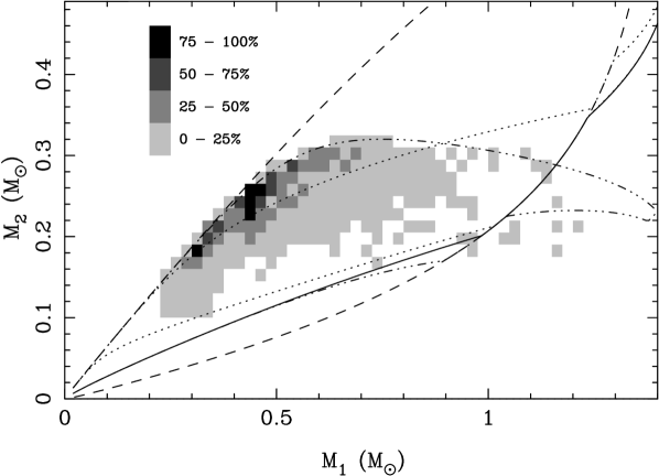
Figure 10: The masses of double white dwarfs at birth from the binary population models of Nelemans et al. (2001) that survive in the case of strong coupling ($\tau_{S}=0$). The surviving models do not reach the limit of guaranteed stability in this case (upper dashed curve) because super-Eddington accretion becomes the more stringent constraint (as marked by the dot–dashed line). Dotted lines are as plotted in Fig. 1

The greyscale only shows systems that can become AM CVn binaries. They concentrate towards the line dividing sub- from super-Eddington systems because they are outliers from the majority of systems which have near-equal mass ratios. This depends upon the physics of the common envelope amongst other things: Nelemans et al. (2001) developed their model partly in response to the observations of equal mass ratios of double white dwarfs. Others have found more unequal distributions (Iben et al. 1997; Han 1998), nevertheless all models so far peak with $q>0.4$ and thus all predict that most systems are unstable and will merge. The high density near the stability limit of Nelemans et al.’s distribution means that the birth rate of AM CVn systems from the double white dwarf path is very sensitive to the strength of synchronisation torque. This can be seen in Fig. 11

Figure 11: The birth rate of AM CVn systems descended from double white dwarfs as a function of the synchronisation timescale at the start of mass transfer. We show also the case for isothermal mass transfer (dotted line) to show that the mass transfer mode has a relatively slight overall effect. The plot was derived from our analytic approximations for speed, but limited comparisons with numerical integrations produced nearly-identical results.

in which we plot the birth-rate (from the double white dwarf merger route) as a function of the synchronisation timescale . This figure shows that as spin–orbit coupling weakens, the birth rate of AM CVn stars from double white dwarfs (which we assume to be equivalent to survival of mass transfer as a binary) drops by about one hundred-fold. A synchronisation timescale $\tau_{S}<1000\,\hbox{yr}$ is enough to increase the birth rate from its lowest value by more than a factor of two. While sensitive to the mass ratio distribution of the detached double white dwarfs, this calculation illustrates the potential significance of dissipative synchronisation torques for the population of AM CVn systems. In this figure we also show the results for isothermal mass transfer, which shows that variations between the two extremes is not that large.

One could hope that an observational estimate of the birth rate of AM CVn stars might decide whether we are in the strong or weak coupling part of Fig. 11. Unfortunately in our opinion, uncertainties and selection effects are too large to allow this to be done. First, there are only two directly-measured distances (GP Com, $68\pm 7\,{\rm pc}$, Thorstensen 2004; AM CVn, $235\,{\rm pc}$, C.Dahn, priv. comm.). The AM CVn distance is a factor of 3 further than Warner (1995) assumed in estimating the space density, which if it applied to all systems would imply an overestimate by a factor of 27, which serves to show how uncertain observational estimates are. To add to this, Nelemans et al. (2001) estimate that while 99% of AM CVns have periods $P>2000\,{\rm sec}$, they will only form $\sim 10$% of the observed sample, an estimate that itself depends upon highly uncertain assumptions about selection. Finally, the models that lead to Fig. 11 have uncertain normalisation – a factor of 5 to 10 seems quite possible. There is clearly considerable scope for work in this area.

6 Discussion

The requirement that the initial synchronisation timescale is below $1000\,\hbox{yr}$ in order to raise survival rates of double white dwarfs as binary systems is the most important result of this paper. There are few calculations of synchronisation of white dwarfs in binaries, but those that exist come nowhere near this strength of synchronisation. For instance, Campbell’s (1984) estimate for radiative damping (Eq. 38) applied to a pair of white dwarfs with masses of $M_{1}=0.5\,\mathrm{M}_{\odot}$ and $M_{2}=0.2\,\mathrm{M}_{\odot}$ gives $\tau_{S}\sim 10^{12}\,\hbox{yr}$. Even longer times ($10^{15}\,\hbox{yr}$, Webbink & Iben 1987) emerge from calculations based upon the viscosity of degenerate matter. Indeed, the estimates of synchronisation timescales are so long that even the mass donor would not have achieved synchronism prior to mass transfer let alone the accretor (Mochkovitch & Livio 1989). If these estimates are reliable, then the lowest birth rate estimates of Nelemans et al. (2001) are to be preferred. However, it is widely recognised by the authors of the papers on synchronisation of white dwarfs that the problem is essentially unsolved: the possibilities of turbulent viscosity (Horedt 1975) and the excitation of non-radial modes (Campbell 1984) can dramatically shorten the synchronisation time. For instance, Mochkovitch & Livio (1989) argue that turbulent viscosity can give synchronisation timescales $\ll 500\,\hbox{yr}$, exactly what is needed to raise the birth rates significantly. The uncertainty over the dissipation mechanisms within white dwarfs is thus a major unsolved problem for AM CVn evolution.

If the synchronisation torques are not strong, then either the ultra-short period systems (if they are such) are descended from systems that have always had extreme enough mass ratios to be stable, or the double white dwarf route may not be the main channel for these systems. The former alternative is possible, despite the absence of a single system of extreme mass ratio amongst the observed close double white dwarf population (Maxted et al. 2002), because they are expected to be rare, as shown by Fig. 10. This would mean that AM CVn birth rates through the double white dwarf route are dependent upon on a so-far-untested part of the mass ratio distribution of double white dwarfs. The main objection to formation other than from two white dwarfs is the relative difficulty of reaching ultra-short orbital periods by other routes: it is important from this point of view that the photometric periods of order 10 minutes or less are confirmed (or not) as orbital periods.

One way to test our ideas would be to establish that there are systems in existence that are stabilised by synchronisation torques. Although such systems are likely to be in a phase of direct impact accretion, it is important to realise that direct impact on its own does not equal instability. There is a region of parameter space of stable, direct impact accretion even in the absence of synchronisation torques (the slim lenticular region in Fig. 1 containing the word “Direct”). For instance, V407 Vul, if it is a direct impact accretor, could be in this region (Marsh & Steeghs 2002); so too could RXJ J0806.3+1527. Thus even if direct impact accretion were to be established in a double white binary, it would not mean that significant synchronising torques were acting. We would need in addition to establish that the system parameters implied instability in the absence of such torques. Short period systems are of particular interest in this respect since short periods require high donor masses, and correspondingly high accretor masses if they are to remain in the lenticular region. This is an excellent reason for attempting to find further examples of such systems. X-ray surveys would seem the most promising method, since both V407 Vul and RX J0806.3+1527 were found in this manner, although in the future perhaps space-based gravitational wave detectors will prove even more useful (Nelemans, Yungelson & Portegies Zwart 2004).

Similar remarks apply to CVs, except for these stars the unstable region of Fig. 9 is small enough that it seems unlikely that the stellar masses can be measured with enough accuracy to be certain that a given system is located within it.

6.1 Measuring synchronisation torques from other binary stars

The strength of synchronisation torques on white dwarfs might be testable in other systems. If any short period systems with rapidly rotating white dwarfs can be identified, it might be possible to place a lower limit upon the synchronisation torque acting. For instance, rotation velocities have been measured for several white dwarfs in CVs (Sion 1999). The strongest constraints come from high spin-rate, low accretion-rate, short-period systems. Perhaps the best example is the cataclysmic variable WZ Sge, which has an orbital period of $81.6\,\min$ and an accretor which shows signs of having a spin period of $\approx 28\,\sec$ (Patterson et al. 1998). WZ Sge is an old, low accretion rate system, accreting via a disc. Assuming that its spin period represents the equilibrium between accretion and tidal dissipation torques, and since $\Omega_{s}\gg\Omega_{o}$, we have

$$\tau_{S}=\frac{kM_{1}R_{1}^{2}\Omega_{s}}{|\dot{M}_{2}|\sqrt{GM_{1}R_{a}}},$$ (41)

where $R_{a}$ is the radius equivalent to the specific angular momentum of the accreted material. We expect $R_{a}$ to lie in the range $R_{1}<R_{a}<R_{h}$ (allowing $R_{a}\neq R_{1}$ because the accretor may be magnetised given the presence of a spin signal). We take for the mass transfer rate $|\dot{M}_{2}|=3\times 10^{-11}\,\mathrm{M}_{\odot}\,\hbox{yr}^{-1}$, estimated from Fig. 1 of Kolb & Baraffe (1999) as we are interested in the long term average value since the timescale turns out to be long. Thus assuming for WZ Sge that $M_{1}=1\,\mathrm{M}_{\odot}$ and $M_{2}=0.08\,\mathrm{M}_{\odot}$ (Steeghs et al. 2001), we find

$$3\times 10^{8}<\tau_{S}<1.4\times 10^{9}\,\hbox{yr}.$$ (42)

Armed with the constraint on $\tau_{S}$ from WZ Sge, we can scale to a double white dwarf with $M_{1}=1\,\mathrm{M}_{\odot}$ and $M_{2}=0.26\,\mathrm{M}_{\odot}$. The separation of such a system is $9.5$ times smaller than WZ Sge, while the donor is $3.25$ times more massive. Scaling according to $\tau_{S}\propto a^{6}M_{2}^{-2}$ ($M_{1}$ and $R_{1}$ being the same), the equivalent range of $\tau_{S}$ for the double white dwarf is

$$40<\tau_{S}<180\,\hbox{yr},$$ (43)

very much the sort of values that can have an impact upon AM CVn evolution.

Unfortunately, there are significant problems with the above analysis. If the pulsation in WZ Sge really does mean that the accretor is magnetic (and truly represents the white dwarf’s spin period), then it may be magnetic coupling to the outer accretion disc which keeps it rotating slowly. In addition there are complications of nova outbursts in CVs which probably make them unsuitable for measurement of $\tau_{S}$ under any circumstances (Livio & Pringle 1998). Detached systems avoid these problems, and perhaps might make it possible to measure a spin-down rate if a weakly-magnetic example could be found (but strong enough to give a spin pulse) and it could be shown that magnetic and accretion torques were negligible. Interestingly there is apparently a detached system which contains a fairly rapid rotator (EC13471-1258, O’Donoghue et al. 2003), but in this case it is suggested that this was caused by a recent episode of accretion, and so it is not an indication of weak synchronisation. We are left with no clear answer as to the strength of synchronising torques from the known types of white dwarf binary stars. Nevertheless, it is clear from the estimate above that if tidal synchronisation is significant for the evolution of AM CVn systems, then it should also be important in fixing the spin rates of white dwarfs in cataclysmic variable stars and similar systems, and this could be a possible explanation for the generally low rotational velocities detected so far in cataclysmic variable stars, none of which are near the break-up rate (Sion 1999).

6.2 Magnetic versus tidal synchronisation

If magnetic rather than tidal torques were dominant, an interesting filtering effect could occur in which systems with strongly magnetic accretors survive mass transfer while non-magnetic systems mostly merge. One would then expect magnetic accretors to be over-represented amongst the AM CVn systems. This is not obviously the case, e.g. GP Com has no detectable circular polarisation (Cropper 1986) and along with V396 Hya shows the clear signature of emission from a disc, while other systems in the class show shallow absorption line spectra similar to those of high-state non-magnetic CVs rather than the magnetic AM Her class. This suggests that either the fraction of merging double white dwarfs that are magnetic is so low that even the pruning of 99 per cent of the non-magnetic systems fails to reveal them, or that tidal synchronisation is effective in stabilising both non-magnetic and magnetic systems, or that neither magnetic nor tidal synchronisation has much effect or, finally, that AM CVn stars do not form through the double white dwarf route.

6.3 Period changes

As several investigators have realised, measurements of period changes have some potential to discriminate between models of the ultra-compact binary stars. Once a system has settled onto its long term evolution towards the AM CVn phase and spin equilibrium has been reached, it is straight-forward to show that the period derivative in a semi-detached state $\dot{P}_{SD}$ relative to its pure GR-driven value when detached $\dot{P}_{D}$, is given by

$$\frac{\dot{P}_{SD}}{\dot{P}_{D}}=\frac{(\zeta_{2}-\zeta_{r_{L}})/2}{1+(\zeta_{2}-\zeta_{r_{L}})/2-q}.$$ (44)

Since $\zeta_{r_{L}}\approx 1/3$ and $\zeta_{2}\approx-1/3$, and since the denominator of the above expression must be positive for stability, this ratio is negative; see Table 1 for some explicit values for systems which are stable even when there are no synchronisation torques.

$M_{1}$	$M_{2}$	$\dot{P}_{SD}/\dot{P}_{D}$	$M_{1}$	$M_{2}$	$\dot{P}_{SD}/\dot{P}_{D}$
$\mathrm{M}_{\odot}$	$\mathrm{M}_{\odot}$		$\mathrm{M}_{\odot}$	$\mathrm{M}_{\odot}$
0.3	0.06	-0.61	0.7	0.08	-0.53
0.5	0.06	-0.52	0.7	0.10	-0.58
0.5	0.08	-0.58	0.7	0.12	-0.64
0.5	0.10	-0.66	0.7	0.14	-0.70
0.7	0.06	-0.48

Table 1: The ratio of the period derivative in a semi-detached state to its value when (just) detached is given for different stellar masses.

To date period changes have been reported for V407 Vul (Strohmayer 2002) and RX J0806.3+1527 (Hakala et al. 2003; Strohmayer 2003), and in each case the period was found to be decreasing. These results favour a detached rather than semi-detached configuration for these two systems (ES Cet on the other hand is clearly accreting). This would weaken the case for V407 Vul and RX J0806.3+1527 having passed through the state discussed in this paper, although period changes in other close binary stars such as the cataclysmic variable stars have proved unreliable as a means of measuring long-term angular momentum changes (Applegate 1992; Baptista et al. 2003). The periods of the ultra-compact systems should continue to be monitored to see whether similar problems affect these stars, although one might hope that at such short periods gravitational wave angular momentum losses will dominate over any secondary effects.

7 Conclusions

We have studied the onset of mass transfer between two white dwarfs, in particular its stability during the phase when the accretion stream hits the accretor directly. We find that this phase can be stabilised by coupling of the spin of the accretor to the binary orbit, through dissipative processes such as tidal stressing and magnetic induction. However, the coupling needs to be strong and must act on a timescale $<1000\,\hbox{yr}$ when mass transfer first starts to have much effect upon the survival rates of the systems. Standard estimates of the synchronisation timescales in white dwarfs are orders of magnitude longer than this, but may wildly underestimate the synchronisation torques. We have also found that during disc accretion, the angular momentum lost to the accretor at the inner edge of disc also destabilises mass transfer, and is almost as significant as the direct impact case, essentially because the radius of the accretor is comparable to the circularisation radius in these systems. The same effect plays a lesser but non-negligible role in non-magnetic cataclysmic variable stars. Further discoveries of ultra-compact double white dwarfs have the potential to tell us whether synchronisation torques are indeed important for surviving this exciting phase of evolution.

Appendix A Quasi-static solutions

In this appendix we are interested in quasi-static solutions of equations 2.2 and 21, “static” on timescales short compared to the secular evolution of the system parameters and their stability. As outlined in section 3.1, we assume therefore that the coefficients involving binary masses and separation are constant.

We define the following dimensionless variables

$$t \rightarrow t/\tau_{S},$$ (45)

$$x = -\tau_{S}\frac{\dot{M}_{2}}{M_{2}},$$ (46)

$$y = \frac{\omega}{\Omega_{o}},$$ (47)

$$z = \frac{\Delta}{2R_{2}},$$ (48)

the first being a rescaling of the timescale. With these new variables, equations 2.2 and 21, can be written as

$$\frac{dz}{dt} = a_{1}-a_{2}y-a_{3}x$$ (49)

$$\frac{dy}{dt} = -a_{4}xy-y+a_{5}x,$$ (50)

where the dimensionless coefficients $a_{1}$ to $a_{5}$ are given by

$$a_{1} = \frac{\tau_{S}}{\tau_{G}},$$ (51)

$$a_{2} = \frac{kr_{1}^{2}(1+q)}{q},$$ (52)

$$a_{3} = 1+\frac{\zeta_{2}-\zeta_{r_{L}}}{2}-q-\sqrt{(1+q)r_{h}},$$ (53)

$$a_{4} = \lambda q,$$ (54)

$$a_{5} = \frac{q\sqrt{(1+q)r_{h}}}{kr_{1}^{2}(1+q)}-\lambda q,$$ (55)

and where $\tau_{G}=-J_{\mathrm{orb}}/\dot{J}_{\mathrm{GR}}$ and $r_{1}=R_{1}/a$ as before. The coefficients $a_{1}$, $a_{2}$ and $a_{5}$ are positive, while $a_{3}$ and $a_{4}$ can be either positive or negative. For Eggleton’s mass-radius relation, Eq. 2.3, for instance, $a_{4}<0$ for $M_{1}>0.40\,\mathrm{M}_{\odot}$.

For the solutions of interest, $\dot{y}=\dot{z}=0$, and we are left with two simultaneous equations

$$a_{3}x_{e}+a_{2}y_{e} = a_{1},$$ (56)

$$a_{5}x_{e}-y_{e} = a_{4}x_{e}y_{e}.$$ (57)

These lead to a quadratic equation with solutions

$$x_{e}=\frac{-b\pm\sqrt{b^{2}+4a_{1}a_{3}a_{4}}}{2a_{3}a_{4}},$$ (58)

where

$$b=a_{3}+a_{2}a_{5}-a_{1}a_{4}.$$ (59)

Solutions of physical interest must have real, positive $x_{e}$, and, for reasons of stability, if there are two such solutions, the smaller of the two is favoured.

This divides parameter space into two parts according to whether there are or are not any solutions. The region where there are solutions is further sub-divided according to whether or not the solutions are stable.

A.1 The dynamically unstable case

We know that $a_{1}>0$. Hence, if $a_{4}>0$ and $a_{3}+a_{2}a_{5}<0$ (which since $a_{2}$ and $a_{5}$ are both positive implies $a_{3}<0$), then $b<0$ and $|b^{2}+4a_{1}a_{3}a_{4}|<|b|$, and so there are no real and positive solutions for $x_{e}$. The condition $a_{3}+a_{2}a_{5}<0$ is equivalent to:

$$q>1+\frac{\zeta_{2}-\zeta_{r_{L}}}{2}-kr_{1}^{2}(1+q)\lambda,$$ (60)

which was quoted in the main text as Eq. 30.

If $a_{4}<0$, as is possible, there is formally a positive solution of Eq. 58, but only at such high spin rates that we run into the break-up limit of the accretor. The consequence is that Eq. 60 remains a good condition for instability.

A.2 The dynamically stable case

The reverse of the unstable case is when $a_{3}>0$, when one can show that there is always a solution for real, positive $x_{e}$, for any $\tau_{S}$ and $a_{4}$. The condition $a_{3}>0$ means that

$$q<1+\frac{\zeta_{2}-\zeta_{r_{L}}}{2}-\sqrt{(1+q)r_{h}},$$ (61)

as derived by Nelemans et al. (2001). As noted in the main text, this can be adapted for disc-fed accretion by replacing $r_{h}$ by $r_{1}=R_{1}/a$.

Systems evolve towards this solution with time since their mass ratios continuously decrease. We will prove below that the equilibrium is stable in this case. Before doing so, we look at the equilibrium mass transfer rate in this stable case. The equations derived here are those used in the comparison of analytical and numerical results shown in Fig. 4.

There are two extreme cases as $\tau_{S}\rightarrow 0$ or $\tau_{S}\rightarrow\infty$. As $\tau_{S}\rightarrow 0$, $a_{1}\rightarrow 0$ and

$$x_{e}\rightarrow\frac{a_{1}}{a_{3}+a_{2}a_{5}}.$$ (62)

Dividing out the $\tau_{S}$ in the definitions of $x$ and $a_{1}$, then we have

$$\frac{-\dot{M}_{2e}}{M_{2}}\longrightarrow\frac{-\dot{J}_{\mathrm{GR}}/J_{\mathrm{orb}}}{1+(\zeta_{2}-\zeta_{r_{L}})/2-q-kr_{1}^{2}\lambda(1+q)}$$ (63)

This is, as expected, the usual expression for stable mass transfer, albeit slightly modified by the term including $kr_{1}^{2}$ as a result of the angular momentum removed from the orbit by the accreting white dwarf owing to its increasing mass. This term contributes at most $\sim 0.01$, and can safely be ignored.

When $\tau_{S}\rightarrow\infty$, we run into break-up of the accretor once more. It is then clear from Eq. 2.5 that the equilibrium mass transfer rate is given by

$$\frac{-\dot{M}_{2e}}{M_{2}}=\frac{-\dot{J}_{\mathrm{GR}}/J_{\mathrm{orb}}}{1+(\zeta_{2}-\zeta_{r_{L}})/2-q-k\lambda\sqrt{(1+q)r_{1}}}.$$ (64)

The final factor in the denominator is again fairly small, and so this mass transfer rate is very similar to that of Eq. 63. Thus we conclude that systems undergoing direct impact accretion which satisfy Nelemans et al.’s (2001) strict stability condition, Eq. 31, always have equilibria with mass transfer rates close to that of Eq. 63.

Nelemans et al. (2001) use a different equation to compute the Eddington-limited mass transfer rate in the stable direct impact case. On their Fig. 1 they plot a dashed line obtained from the relation

$$\frac{-\dot{M}_{2e}}{M_{2}}=\frac{-\dot{J}_{\mathrm{GR}}/J_{\mathrm{orb}}}{1+(\zeta_{2}-\zeta_{r_{L}})/2-q-\sqrt{(1+q)r_{h}}}$$ (65)

which gives substantially higher mass transfer rates than either of Eqs 63 and 64. Although this is not the equilibrium rate, Nelemans et al. were in fact correct to use this, at least in the weak coupling case, as can be seen by considering the situation that applies as $\tau_{S}\rightarrow\infty$ while $\omega$ remains finite. Eq. 2.2 then becomes

$$\frac{1}{2R_{2}}\frac{d\Delta}{dt}=-\frac{\dot{J}_{\mathrm{GR}}}{J_{\mathrm{orb}}}+\left(1+\frac{\zeta_{2}-\zeta_{r_{L}}}{2}-q-\sqrt{(1+q)r_{h}}\right)\frac{\dot{M}_{2}}{M_{2}},$$ (66)

and the equilibrium solution, $\dot{\Delta}=0$, gives Eq. 65. Although this a temporary state that will stop once the white dwarf has spun up to break-up, it is still long-lasting (see Fig. 4). The spin-up phase will last a time $\tau_{B}$ given by

$$\frac{\tau_{B}}{\tau_{G}}\approx k\sqrt{r_{1}/r_{h}}(1+(\zeta_{2}-\zeta_{r_{L}})/2-q-\sqrt{(1+q)r_{h}}),$$ (67)

which can be long enough for the system to switch to disc accretion, although once break-up is reached, the mass transfer rate is still given by Eq. 64. These results are the ones illustrated graphically in Fig. 4. As spin–orbit coupling increases we expect a peak rate intermediate between that given by Eq. 64 and that given by Eq. 65.

A.3 Stability of Equilibrium

The case of most interest to us is when the mass ratio lies in between the unstable and stable limits of Eqs 60 and 61 when $-a_{2}a_{5}<a_{3}<0$. In this case synchronisation can bring about an equilibrium solution which disappears as $\tau_{S}\rightarrow\infty$. This then sets an upper limit on $\tau_{S}$ required for the existence of an equilibrium solution. However it turns out that an even stricter constraint comes from the requirement that the equilibrium solution be stable. This is a new feature: so far there either have been or there have not been equilibrium solutions, and if they existed we have implicitly assumed that they were stable equilibria. We now come across equilibrium solutions that can be stable or unstable.

Consider the following small perturbations from equilibrium:

$$y = y_{e}+y^{\prime},$$ (68)

$$z = z_{e}+z^{\prime},$$ (69)

$$x = x_{e}+\beta x_{e}z^{\prime},$$ (70)

where in the last equation we recognize that $x$ varies with $z$ alone since the mass transfer rate depends explicitly upon $\Delta$ but not $\omega$, and the dimensionless factor $\beta$ is defined by

$$\beta=2R_{2}\frac{d\log(-\dot{M}_{2})}{d\Delta}.$$ (71)

Since the mass transfer rate increases monotonically with $\Delta$, $\beta$ is positive. For the two mass loss models we consider in section 2.2

$$\beta_{i}=2\frac{R_{2}}{H},$$ (72)

for the isothermal case of Eq. 8, and

$$\beta_{a}=6\frac{R_{2}}{\Delta_{e}},$$ (73)

for the adiabatic case of Eq. 9, where $\Delta_{e}$ is the equilibrium value of the overfill factor; it is the latter expression that we employed throughout the paper.

Applying the perturbation to Eqs 49 and 50 while keeping terms to first order in the small dashed quantities gives

$$\dot{z^{\prime}} = -\beta x_{e}a_{3}z^{\prime}-a_{2}y^{\prime},$$ (74)

$$\dot{y^{\prime}} = \beta x_{e}(a_{5}-a_{4}y_{e})z^{\prime}-(1+a_{4}x_{e})y^{\prime}.$$ (75)

These are two first-order, coupled equations. Assuming solutions of the form $e^{pt}$, one obtains an eigenvalue equation for $p$ with values that are solutions of the following quadratic:

$$p^{2}+\left(1+a_{4}x_{e}+\beta x_{e}a_{3}\right)p+\beta\left(a_{1}+a_{3}a_{4}x_{e}^{2}\right)=0.$$ (76)

after using Eqs 56 and 57 to simplify the third term. The solutions are stable provided that $\mathrm{Re}(p)<0$ for both roots. This is true if the two coefficients of the quadratic are both positive. The coefficient of the term linear in $p$ is positive if

$$\frac{1}{\tau_{S}}>-\left[a_{3}\beta+a_{4}\right]\frac{-\dot{M}_{2e}}{M_{2}},$$ (77)

or, when written out in full,

$$\frac{1}{\tau_{S}} > -\left[\left(1+\frac{\zeta_{2}-\zeta_{r_{L}}}{2}-q-\sqrt{(1+q)r_{h}}\right)\beta\right.$$

$$\;\;\;\;\;\;+\left.q\lambda\rule{0.0pt}{11.38109pt}\right]\frac{-\dot{M}_{2e}}{M_{2}},$$

which was quoted in the main text (Eq. 32). It turns out that the coefficient of the constant term is also positive when this condition is satisfied, so no further restriction is necessary. Eq. A.3 is a generalisation of Nelemans et al.’s (2001) strict condition for stability (Eq. 31) and is the key result of this paper. Eq. A.3, derived from the condition, $a_{3}\beta+a_{4}>0$, does not quite match the criterion for stability regardless of $\tau_{S}$, Eq. 61, which corresponds to $a_{3}>0$. This is because Eq. A.3 permits arbitrarily high rates of spin, whereas in reality the spin rate is limited by break-up. Both criteria are correct, but under different conditions: Eq. 61 applies in the case of zero synchronisation, while Eq. A.3 applies when there are synchronising torques strong enough to keep the spin rate of the accretor below the break-up rate.

References

- [1] Alexander M. E., 1973, Ap&SS, 23, 459
- [2] Applegate J. H., 1992, ApJ, 385, 621
- [3] Baptista R., Borges B. W., Bond H. E., Jablonski F., Steiner J. E., Grauer A. D., 2003, MNRAS, 345, 889
- [4] Campbell C. G., 1983, MNRAS, 205, 1031
- [5] Campbell C. G., 1984, MNRAS, 207, 433
- [6] Chandrasekhar S., 1967, An introduction to the study of stellar structure, New York: Dover
- [7] Cropper M., 1986, MNRAS, 222, 225
- [8] Cropper M., Harrop-Allin M. K., Mason K. O., Mittaz J. P. D., Potter S. B., Ramsay G., 1998, MNRAS, 293, L57
- [9] Deloye C. J., Bildsten L., 2003, ApJ, 598, 1217
- [10] Eggleton P. P., 1983, ApJ, 268, 368
- [11] Eggleton P. P., Kiseleva L. G., Hut P., 1998, ApJ, 499, 853
- [12] Hakala P., Ramsay G., Wu K., Hjalmarsdotter L., Järvinen S., Järvinen A., Cropper M., 2003, MNRAS, 343, L10
- [13] Han Z., 1998, MNRAS, 296, 1019
- [14] Han Z., Webbink R. F., 1999, A&A, 349, L17
- [15] Horedt G., 1975, A&A, 44, 461
- [16] Iben I.Jr., Tutukov A.V., 1984, ApJ Supp, 54, 335
- [17] Iben I.Jr., Tutukov A.V., Yungelson L.R., 1997, ApJ, 475, 291
- [18] Iben I. J., 1990, ApJ, 353, 215
- [19] Iben I. J., Tutukov A. V., 1991, ApJ, 370, 615
- [20] Iben I. J., Tutukov A. V., Fedorova A. V., 1998, ApJ, 503, 344
- [21] Israel G. L. et al., 2002, A&A, 386, L13
- [22] Koester D., 1980, A&AS, 39, 401
- [23] Kolb U., Baraffe I., 1999, MNRAS, 309, 1034
- [24] Landau L. D., Lifshitz E. M., 1975, The classical theory of fields, Oxford: Pergamon Press, 1975
- [25] Livio M., Pringle J. E., 1998, ApJ, 505, 339
- [26] Marsh T.R., Dhillon V.S., Duck S.R., 1995, MNRAS, 275, 828
- [27] Marsh T. R., Steeghs D., 2002, MNRAS, 331, L7
- [28] Maxted P. F. L., Marsh T. R., Moran C. K. J., 2002, MNRAS, 332, 745
- [29] Meyer F., Meyer-Hofmeister E., 1983, A&A, 121, 29
- [30] Mochkovitch R., Livio M., 1989, A&A, 209, 111
- [31] Motz L., 1952, ApJ, 115, 562
- [32] Napiwotzki R. et al., 2003, White Dwarfs, proceedings of the conference held at the Astronomical Observatory of Capodimonte, Napoli, Italy. To be published by Kluwer. (NATO Science Series II – Mathematics, Physics and Chemistry, Vol. 105, p. 39.)
- [33] Nather R. E., Robinson E. L., Stover R. J., 1981, ApJ, 244, 269
- [34] Nauenberg M., 1972, ApJ, 175, 417
- [35] Nelemans G., Portegies Zwart S. F., Verbunt F., Yungelson L. R., 2001, A&A, 368, 939
- [36] Nelemans G., Yungelson L. R., Portegies Zwart S. F., 2004, MNRAS, in press, astro-ph/0312193
- [37] O’Donoghue D., Koen C., Kilkenny D., Stobie R. S., Koester D., Bessell M. S., Hambly N., MacGillivray H., 2003, MNRAS, 345, 506
- [38] Paczyński B., 1971, ARA&A, 9, 183
- [39] Paczyński B., Sienkiewicz R., 1972, Acta Astr., 22, 73
- [40] Patterson J., Richman H., Kemp J., Mukai K., 1998, PASP, 110, 403
- [41] Podsiadlowski P., Han Z., Rappaport S., 2003, MNRAS, 340, 1214
- [42] Priedhorsky W. C., Verbunt F., 1988, ApJ, 333, 895
- [43] Ramsay G., Wu K., Cropper M., Schmidt G., Sekiguchi K., Iwamuro F., Maihara T., 2002, MNRAS, 333, 575
- [44] Ramsay G., Hakala P., Cropper M., 2002, MNRAS, 332, L7
- [45] Rieutord M., Bonazzola S., 1987, MNRAS, 227, 295
- [46] Ritter H., 1988, A&A, 202, 93
- [47] Saio H., Jeffery C. S., 2002, MNRAS, 333, 121
- [48] Savonije G. J., 1978, A&A, 62, 317
- [49] Sion E.M., 1999, PASP, 111, 532
- [50] Steeghs D., Marsh T., Knigge C., Maxted P. F. L., Kuulkers E., Skidmore W., 2001, ApJL, 562, L145
- [51] Strohmayer T. E., 2002, ApJ, 581, 577
- [52] Strohmayer T. E., 2003, ApJL, 593, L39
- [53] Thorstensen J. R., 2004, AJ, in press, astro-ph/0308516
- [54] Tutukov A., Yungelson L., 1996, MNRAS, 280, 1035
- [55] Verbunt F., Rappaport S., 1988, ApJ, 332, 193
- [56] Warner B., 1995, Cataclysmic variable stars, Cambridge Astrophysics Series, Cambridge, New York: Cambridge University Press
- [57] Warner B., Woudt P. A., 2002, PASP, 114, 129
- [58] Webbink R.F., 1979, IAU Colloq. 53: White Dwarfs and Variable Degenerate Stars
- [59] Webbink R.F., 1984, ApJ, 277, 355
- [60] Webbink R. F., 1977, ApJ, 211, 486
- [61] Webbink R. F., Iben I. J., 1987, IAU Colloq. 95: Second Conference on Faint Blue Stars
- [62] Wu K., Cropper M., Ramsay G., Sekiguchi K., 2002, MNRAS, 331, 221
- [63] Zahn J.-P., 1977, A&A, 57, 383
- [64] Zapolsky H. S., Salpeter E. E., 1969, ApJ, 158, 809