Chandra High-Resolution X-Ray Spectrum of Supernova Remnant 1E 0102.2-7219

Abstract

Chandra High Energy Transmission Grating Spectrometer observations of the supernova remnant 1E 0102.2-7219 in the Small Magellanic Cloud reveal a spectrum dominated by X-ray emission lines from hydrogen-like and helium-like ions of oxygen, neon, magnesium and silicon, with little iron. The dispersed spectrum shows a series of monochromatic images of the source in the light of individual spectral lines. Detailed examination of these dispersed images reveals Doppler shifts within the supernova remnant, indicating bulk matter velocities on the order of 1000 km s^-1. These bulk velocities suggest an expanding ring-like structure with additional substructure, inclined to the line of sight. A two-dimensional spatial/velocity map of the SNR shows a striking spatial separation of redshifted and blueshifted regions, and indicates a need for further investigation before an adequate 3D model can be found. The radii of the ring-like images of the dispersed spectrum vary with ionization stage, supporting an interpretation of progressive ionization due to passage of the reverse shock through the ejecta. Plasma diagnostics with individual emission lines of oxygen are consistent with an ionizing plasma in the low density limit, and provide temperature and ionization constraints on the plasma. Assuming a pure metal plasma, the mass of oxygen is estimated at $\sim$6 M_⊙, consistent with a massive progenitor.

1 Introduction

The SNR 1E 0102.2-7219 (E0102) is a well studied member of the oxygen rich class of supernova remnants located in the Small Magellanic Cloud (SMC). Gaetz et al. (2000) reported spectrally resolved imaging from Chandra’s ACIS detector, which shows an almost classic, text-book SNR with a hotter outer ring identified with the forward shock surrounding a cooler, denser inner ring which is presumably the reverse-shocked stellar ejecta. Hughes et al. (2000b) combined the Chandra image with earlier Einstein and ROSAT images to measure X-ray proper motions, which give an expansion age of $\sim$1000 yr, consistent with earlier estimates based on optical measurements of oxygen-rich material (Tuohy & Dopita, 1983; Dopita et al., 1981; Hayashi et al., 1994; Gaetz et al., 2000). By contrast, Eriksen et al. (2001) estimate a free expansion age of 2100 years. Hughes et al. (2000b) deduce that a significant fraction of the shock energy has gone into cosmic rays. Composite X-ray spectra of moderate resolution have been obtained for the whole remnant with ASCA (Hayashi et al., 1994) and XMM–Newton (Sasaki et al., 2001). These observations confirm that a single component non-equilibrium plasma is inadequate to account for the global SNR spectrum. A high resolution X-ray spectrum obtained with the reflection grating spectrometer of XMM–Newton reveals a wealth of individual lines of C, O, Ne, Mg and Si (Rasmussen et al., 2001). Line ratios from these spectra confirm non-equilibrium ionization (NEI) conditions consistent with an ionizing plasma in the low density limit.

We report on the high resolution X-ray spectrum of 1E 0102.2-7219 obtained with the Chandra High Energy Transmission Grating Spectrometer; a portion of the spectrum is shown in Figure 1 (preliminary reports were presented in Flanagan et al. (2001); Canizares et al. (2001); Flanagan et al. (2003)). Individual X-ray lines of oxygen, neon, magnesium and silicon echo the sharply defined ring structure seen in direct Chandra images. Notably weak are lines of highly ionized iron. This lack of strong iron lines is fortuitous, since the X-ray spectra of SNRs are commonly dominated (and complicated) by an “iron forest” of lines between 7 Å and 18 Å. The spatial and spectral signatures of E0102 make it a unique candidate for the HETG – bright, sharp spatial features arrayed in a narrow ring around a sparsely filled interior, combined with a spectrum dominated by a relatively small number of discrete lines. As a result, the HETG dispersed line images have only a small amount of overlap between them, enabling straightforward analysis of the individual lines.

The analysis we present follows four broad areas: spectral lines and line fluxes, ionization structure, Doppler shifts and three-dimensional modeling. Section 2 describes the observations and data processing. Section 3 introduces the spectrum, identifies line series, presents line images (Section 3.1), and discusses flux measurements (Section 3.2) which can be cleanly obtained through the relative simplicity of the dispersed spectrum. We follow this with a discussion of plasma diagnostics (Section 3.3) and an estimate of oxygen ejecta mass and associated progenitor models (Section 3.4). Section 4 addresses the ionization structure of the SNR, and relates it to passage of the reverse shock through the ejecta. Section 5 outlines the analysis of Doppler shifts, beginning with techniques and measurements on specific sectors of the SNR, and branching out (Section 5.4) to a Doppler velocity imaging technique which yields a “Doppler map” of the entire SNR. Section 6 introduces a simple three-dimensional model as a first attempt to account for the spatial and velocity structure of the SNR. Sections 7 and 8 discuss and summarize the findings.

2 Observations and Data Analysis

The supernova remnant E0102 was observed with the Chandra High Energy Transmission Grating Spectrometer (HETGS) (Canizares et al., 2000, 2003) in two observation intervals as part of the guaranteed time observation program. Details of the observation are given in Table 1. The instrument configuration included HETG with the Advanced CCD Imaging Spectrometer (ACIS-S) (Garmire et al., 2003; Burke et al., 1997). These two observations of 1E 0102.2-7219 had slightly different roll angles and aim points and were independently treated in our analysis.

The data were processed using standard CXC pipeline software (version R4CU5UPD8.2), employing calibration files available in February, 2001. Processing of the data included running acis_process_events to correctly assign ACIS pulse height to the events (needed for proper order sorting), and filtering the data for energy, status and grade (0,2,3,4,6). Since the supernova remnant is extended, a customized region mask was created to ensure that all source photons were captured, both in the zeroth order (undispersed) image and along the dispersion axes. Further processing included aspect correction, selection of good time intervals, removal of detector artifacts (hot pixels and streaks), and selection of first order photons. At the end of processing, the net live time was 135.5 ks, the bulk of it (86.9 ks) from the first observation interval, Obsid 120.

The HETG consists of two independent sets of gratings with dispersion axes oriented at angles that differ by $\sim$10^∘. The medium energy gratings (MEG) cover an energy range of 0.4 – 5 keV and have half the dispersion of the high energy gratings (HEG), which provide simultaneous coverage of the range 0.9 – 10 keV. The gratings form an undispersed image at the pointing position (the zeroth order image) with Chandra’s full spatial resolution, and with spectral information limited to the moderate resolution provided by the ACIS detector. The dispersed photons provide the high resolution spectrum. The different dispersion directions and two dispersion wavelength scales provide redundancy as well as a means of resolving spectral/spatial confusion problems associated with extended sources such as supernova remnants (discussed in more detail in Section 5). The high resolution spectra from +1 and $-1$ orders are discriminated from overlapping higher orders by using the moderate energy resolution of the ACIS-S. Further details of the instrument can be found in Markert et al. (1994), Chandra Proposers’ Observatory Guide (2002) and at http://space.mit.edu/HETG.

After eliminating higher orders, approximately 47% of the detected photons in the spectrum were in zeroth order, 40% in MEG $\pm$1 orders, and 13% in HEG $\pm$1 orders. The MEG $-1$ order had a higher count rate than the +1 order, attributable to the presence of a backside illuminated CCD, which has much higher detection efficiency for the bright, low energy oxygen lines than the frontside illuminated CCD used in the +1 order. The approximate breakdown of dispersed and undispersed photons in the spectrum is shown in Table 1.

3 The High Resolution X-ray Spectrum

Figure 1 shows a portion of the high resolution spectrum from the $-1$ order of the MEG gratings, taken during the first observation interval, Obsid 120. The dispersed spectrum is analogous to a spectro-heliogram, showing a series of monochromatic images of the source in the light of individual spectral lines. The HETGS spectrum is dominated by lines of highly ionized oxygen, neon and magnesium from ionization stages in which only one (hydrogen-like) or two (helium-like) electrons remain. These are states which are long-lived under conditions typical of supernova remnants. Also present is a helium-like line of silicon (truncated from Figure 1), but notably weak are lines of highly ionized iron (i.e., Fe XVII and Fe XVIII). Relative to the strong lines in the spectrum, the continuum component is weak.

The spectrum reveals multiple lines from the various ions. Several of these transitions are indicated in Figure 2. The hydrogen-like oxygen lines indicate transitions from upper levels n = 2, 3, 4, 5 to n = 1 (i.e., O VIII Lyman $\alpha$, $\beta$, $\gamma$, and $\delta$, respectively). The hydrogen-like neon lines include n = 2, 3, 4 to n = 1 transitions (Ne X Lyman $\alpha$, $\beta$, and $\gamma$). The helium-like oxygen (O VII) and neon (Ne IX) lines include the n = 2, 3, 4 to n = 1 transitions. In each case, the triplet of lines from n = 2 to n = 1 is characterized by bright forbidden (1$s^{2}$ ${}^{1}S_{0}$ – 1s2s ${}^{3}S_{1}$) and resonance lines (1$s^{2}$ ¹S₀ – 1s2p ${}^{1}P_{1}$) and a weak intercombination line (1$s^{2}$ ${}^{1}S_{0}$ – 1s2p ${}^{3}P_{2,1}$). For the hydrogen-like magnesium ion (Mg XII), only n = 2, 3 to n = 1 transitions are detected, and for the helium-like magnesium (Mg XI), n = 2, 3, 4 to n = 1 transitions are detected. Finally, the helium-like Si XIII transition from n = 2 to n = 1 is detected. Note that the silicon transition and fainter magnesium transitions are not marked in Figure 2.

Lines of L-shell transitions of Fe, often quite strong in SNR spectra, are weak in the E0102 spectrum. (Locations where bright Fe lines would typically appear are depicted in Figure 2, illustrating the relative weakness of these lines in the HETG spectrum. The most prominent candidate Fe XVII line was 17.05 Å. Its observed flux was comparable to the continuum level there.) Rasmussen et al. (2001) report a low iron-to-oxygen abundance ratio and conclude that the Fe L lines trace the swept-up ISM rather than the ejecta. This echoes the interpretation by Hayashi et al. (1994) that the iron emission is due to the forward shock interacting with the ISM.

3.1 Line Images

The dispersed spectrum of E0102 shows the two-dimensional structure of the SNR in several prominent lines. Figure 3 shows the undispersed zeroth order image of the SNR (all energies have been included.) The morphology of the remnant (Gaetz et al., 2000) is that of a ring with significant brightness variations. The image shows a bright knot in the southwest with a radial extension or “spoke”, a bright arc in the southeast, and a bright linear feature or “shelf” to the north. These features are visible to various degrees in the dispersed X-ray line images. Also evident in the zeroth order image is the boundary of the outward-moving blast wave noted by Gaetz et al. (2000).

Although the distinctive ring structure of the SNR is echoed in each X-ray line, close inspection reveals differences line-by-line. The dispersed images of prominent lines from the MEG $-1$ order are shown with a uniform spatial scale and 2-pixel Gaussian smoothing in Figure 4. The helium-like triplet is shown to the left and the hydrogen-like Lyman $\alpha$ is to the right for oxygen (top), neon (middle) and magnesium (bottom), respectively.

A comparison of the two oxygen images in the top row of Figure 4 reveals a similar shape but a marked disparity in ring diameter between the two ionization stages. This size difference is taken to be an indicator of the progress of the reverse shock with respect to the ejecta (Gaetz et al., 2000; Flanagan et al., 2001), and is the subject of Section 4. For both oxygen and neon, the forbidden and resonance lines of the helium-like triplets are prominent and easily resolved, providing potentially useful temperature diagnostics, as discussed in Section 3.3.1.

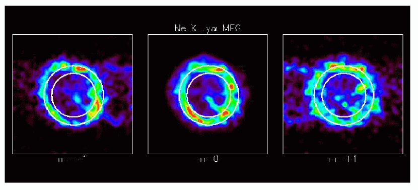
Figure 11: Distortion is evident when dispersed images of Ne X Lyman $\alpha$ are compared with the zeroth order (filtered on the energy of the line). The leftmost panel shows the MEG -1 order ring, the middle panel is the zeroth order, and the right panel is the MEG +1 order ring. Overlaid on these images are alignment rings to assist in identifying distortions. The sharpness of the -1 order ring relative to +1 order indicates the presence of both red- and blueshifts.

Distortions of the SNR ring shape can be seen by comparing the ring from the Ne X Lyman $\alpha$ line, to the right in the middle row of Figure 4, with the undispersed image of Figure 3. In Section 5 (Figure 11), these images are compared with the +1 order, providing compelling evidence for Doppler velocities of the ejecta in the SNR.

The two magnesium images in the bottom row of Figure 4 show a striking difference in that the bottom portion of the ring (i.e., the southeast arc that is so prominent in other images) is virtually missing in the image formed by the hydrogen-like Lyman $\alpha$ line. Given that the Mg XI triplet is detected in the southern half (forming a complete ring), the lack of the Mg XII line cannot be due to absence of the element magnesium, but instead suggests insufficient ionization. The signal-to-noise of the Si XIII image was insufficient to include it in Figure 4. Nevertheless, numerical comparison shows the bottom portion suppressed relative to the top, analogous to the case of Mg XII. Thus, these images indicate the magnesium and silicon plasma to be more highly ionized in the north relative to the south of the SNR. This is discussed more fully in Section 3.3.5.

3.2 Flux Measurements

The usual approach for measuring line fluxes involves folding a spectral emission model through a response matrix and fitting several components simultaneously. However, there is so little overlap in the dispersed line images of the Chandra HETGS spectrum that we have adopted a more straightforward analysis of the individual lines. The measured values are given in Table 2 and the techniques are described below.

The count rate for each bright X-ray line was obtained by using an annular aperture that enclosed the observed ring. (The annular aperture excluded much of the contribution by the “spoke”, representing typically less than 5%. This was generally negligible compared to the errors. For measurements of the oxygen and neon triplets, an elliptical aperture was employed which captured the “spoke” contribution.) The background was taken from regions immediately above and below the line of interest. In both cases, an appropriate PI filter on ACIS energy was used to minimize unwanted events. For the line data presented here the background was a small fraction of the total flux and was much smaller than the error due to photon counting statistics.

In some cases, the dispersed lines overlap other nearby lines (i.e., the forbidden and resonance lines in Figure 4), so that assignment of events between the two X-ray lines is ambiguous. In order to account for this, we extracted the events in a sub-aperture devoid of overlap with the nearby contaminating line. The measurement was then scaled up to obtain an estimate for the full aperture. In making this correction, we took into account the fact that the SNR brightness varies significantly around the ring. We employed the zeroth order image filtered closely on the energy of interest, and assumed that the distribution of events in the sub-aperture relative to the full aperture was the same for the dispersed ring as for this filtered zeroth order image. Accounting for surface brightness variations gives a result within 10% of that derived assuming a uniform surface brightness.

For each of the observation intervals, Obsid 120 and Obsid 968, there are up to four independent flux measurements that may be obtained: MEG +1 and $-1$ orders, and HEG +1 and $-1$ orders. Where feasible, each of these measurements was made. The best counting statistics were obtained with the MEG spectrum. Nevertheless, differences between raw measurements tended to be greater than expected from counting statistics alone, and are attributed to residual calibration effects. In-flight calibration measurements suggest systematic efficiency differences between backside-illuminated and frontside-illuminated CCDs, and differences between HEG and MEG grating measurements. To account for these calibration effects, we have increased individual flux measurements of X-ray lines falling on frontside CCDs by 4–19%. (See http://space.mit.edu/ASC/calib/hetgcal.html. Backside CCD measurements are believed to be correct, so that only frontside measurements were adjusted in this way.) We have also adjusted the individual flux measurements of lines measured with HEG by 2–8% to normalize them to MEG measurements (see Chandra Proposers’ Observatory Guide (2002), Figure 8.26. Note that normalizing the HEG measurements to MEG is an arbitrary choice, as it is currently unknown which represents the correct standard.) Since several such individual measurements are used to determine the flux for each X-ray line reported in Table 2, the impact of these corrections is effectively smaller, typically ranging from 2–10% for frontside CCD correction and $\pm$2% for HEG correction. The resultant overall correction factors (weighted by source counts) are given in Table 2. The largest calibration correction factor is less than 10%.

To empirically estimate the continuum, we extracted regions of the dispersed spectrum where X-ray line images were absent, and applied an absorbed Bremsstrahlung fit. The best-fit model was then used to estimate the continuum contribution for individual line energies nearby. We found that line-free regions longward of the O VII triplet, and between the O VII triplet and O VIII Lyman $\alpha$, could be fit and the continuum contribution in that region (i.e. for lines below $\sim$ 0.7 keV) could be estimated by an absorbed bremsstrahlung model with k$T_{e}$ $\sim$0.9 and $N_{H}=8\times 10^{20}$ cm^-2 (solar abundances). We found that the estimated continuum contribution at the various oxygen line energies agreed well with continuum estimates obtained from an independent fit to whole-spectrum ACIS data by Plucinsky et al. (2001). We took the error in our continuum estimates to be 20% based on typical differences among estimates obtained by these and similar model fits. (For the case of O VIII Lyman $\gamma$, which lies rather far outside the energy range bracketed by the line-free regions, we have enlarged the error to account for the uncertainty in the model there.) We estimate that the continuum contributes less than 10% to the measured flux at the bright lines of the O VII triplet and O VIII Lyman $\alpha$, but more than 20% of the measurement for the weaker oxygen lines (i.e., O VII (1s-3p), O VIII Lyman $\beta$ and O VIII Lyman $\gamma$). We could not obtain a reliable continuum estimate at the energies of the neon, magnesium and silicon lines, as the model we use in the oxygen line region overpredicts the continuum at higher energies. Further work is needed to refine our estimates and to correct the other lines for their continuum component.

Table 2 lists the mean values of the corrected measurements for the set of lines bright enough to be measured by this technique; the error bars in the table reflect the scatter among the individual measurements in addition to the statistical errors. Also listed is the estimated contribution to this measurement due to the continuum, and the net result after subtracting the continuum component.

3.3 Plasma Diagnostics

High resolution grating spectra provide a means to probe plasmas using individual X-ray lines. Ratios formed from different lines of the same element serve as particularly useful plasma diagnostics because they eliminate the impact of uncertainties in abundance or distance. If lines from the same ion are selected, dependence on the relative ionization fractions is reduced. (This provides, for example, a useful diagnostic for electron temperature.) By selecting lines that are close in energy, the impact of uncertainties in the column density is minimized.

Rasmussen et al. (2001) reported the integrated high-resolution spectrum of E0102 from the RGS of XMM–Newton, and employed several line ratios as temperature diagnostics. In addition to the lines evident in the HETGS spectrum, the RGS spectrum revealed lines of hydrogen-like carbon, and marked the absence of nitrogen. (These lines fall outside the HETG energy range.)

Based on the images of Figure 4 and the discussion of Section 3.1, the plasma conditions for magnesium and silicon are distinctly different in the northern and southern portions of the remnant. Plasma diagnostics from ratios of integrated flux measurements for these elements cannot be expected to give a meaningful result. However, the neon and oxygen images in Figure 4 do not exhibit this obvious inhomogeneity, and integrated fluxes might be applicable. The disparity in oxygen ring sizes seen in Figure 4 indicates that the emission regions are different for the two ionization stages (as discussed in Section 4.1). However, a plasma model which accounts for such an evolving ionization state can in principle accommodate this radial dependence. We have employed such a model to assess plasma conditions based on oxygen line ratios.

Table 3 lists useful diagnostic line ratios obtained from oxygen fluxes in Table 2. These have been corrected for underlying continuum. Ratios of neon and magnesium lines are not included because of the uncertainties that remain in estimating and subtracting the underlying continuum component. The raw ratio of observed fluxes (uncorrected for absorbing column) is given in Table 3, followed by the ratio emitted at the source assuming a column density of $N_{H}$ = $8\times 10^{20}$ cm^-2 with solar abundances (Hayashi et al., 1994; Blair et al., 1989). This allows direct comparison with the XMM–Newton results (Rasmussen et al., 2001). The 90% confidence contours are listed in the last column.

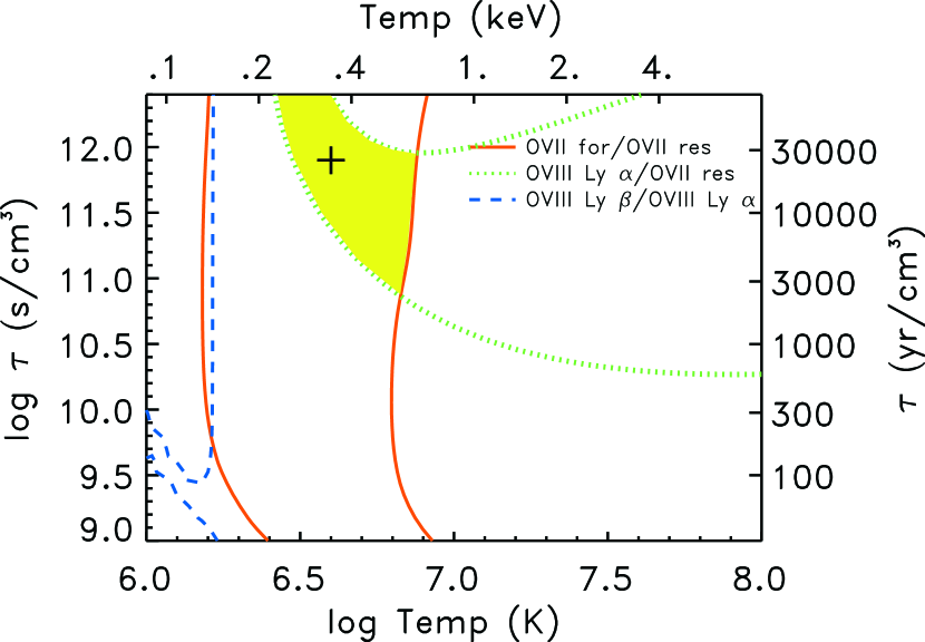
Figure 5: The 90% confidence contours are plotted for line ratios of the brightest measured O VII and O VIII lines, as expected from a plane parallel shock model with input parameters of $T_{e}$, $\tau=\tau_{\rm upper}$. The model (vnpshock) assumes $T_{e}$ = $T_{i}$, and a column density of $N_{H}=8\times 10^{20}cm^{-2}$ with solar abundances. Some flux captured in the forbidden line measurement is actually contributed by a nearby satellite line. The plotted contour accommodates this contribution. The best-fit model is marked by a cross.

We employed a non-equilibrium ionization collisional plasma model from XSPEC version 11.1 (Arnaud, 1996) to calculate expected line ratios. The model, vnpshock (Borkowski et al., 2001), is a plane-parallel shock model that allows the user to select separate electron and ion temperatures. The ionization timescale, $\tau$, which defines the progress of the plasma towards equilibrium, assumes a range of values between lower and upper limits. (The evolution of the plasma is mediated by collisions: $\tau$ equals the product of elapsed time and electron density, and has units of s cm^-3.) By incorporating a range of $\tau$, the model takes into account the evolving nature of the ionization. (We opted not to use another XSPEC non-equilibrium ionization model, NEI, because it assumes a single fixed $\tau$.) We set $\tau_{\rm lower}=0$, and additionally set the ion temperature equal to the electron temperature. (We generally found the diagnostic ratios were dictated by electron temperature, regardless of how the energy was partitioned between the electrons and ions.) We used ISIS (Houck & DeNicola, 2000) to run the XSPEC model and generate tables of expected line ratios. Figure 5 shows the ranges of $T_{e}$ and $\tau=\tau_{\rm upper}$ from the vnpshock model that are compatible with the 90% confidence limits for key line ratios listed in Table 3.

3.3.1 O VII line ratios

Ratios of lines that are close in energy are relatively insensitive to the value of $N_{H}$. Thus, the lines of the O VII triplet can provide particularly valuable diagnostics. However, the faint O VII intercombination line flux cannot be measured by the techniques of Section 3.2, which complicates the analysis. We fitted the components of the triplet using a technique described in Section 5.4, to best determine the proportion of this line in relation to the forbidden and resonance lines of the O VII triplet. The results are shown in Table 4 and corresponding ratios are listed in Table 5. The error for the fluxes obtained by this fitting technique is estimated at $\sim$20%. Within these errors, the values agreed with the fluxes reported in Table 2 for the O VII resonance and forbidden lines.

The HETGS O VII line ratios were found to provide a set of self-consistent temperature diagnostics and are compatible with a single temperature in the range of $\sim$0.14 – 0.77 keV (i.e., 6.2 $<$ log $T_{e}$ $<$ 6.95). The constraining ratio is shown in Figure 5 as the forbidden-to-resonance ratio. The remaining O VII ratios are compatible with this allowed region, and do not further constrain it. Their contours are not plotted. The electron temperature range allowed by the O VII ratios is in agreement with the results obtained with XMM–Newton RGS spectra, where O VII line ratios ($\alpha$$/$$\beta$ and $\beta$$/$$\gamma$ for helium-like oxygen; Rasmussen et al. (2001)) indicate a range of 0.35 $<$ $T_{e}$ $<$ 0.7 keV based on a HULLAC (Bar-Shalom et al., 1988; Klapisch et al., 1977) model for an underionized plasma.

The forbidden (f), intercombination (i) and resonance (r) lines provide other useful diagnostics: R = f/i probes electron density, and G = (i+f)/r can indicate departures from ionization equilibrium (Pradhan, 1982). The measured values for these ratios are given in Table 5. The corresponding XMM–Newton measurements (Rasmussen et al., 2001) are also listed for comparison. Both diagnostic ratios agree with XMM’s observed values. R is consistent with the value expected in the limit of low electron density, and G is compatible with an ionizing plasma (i.e., recombination suppressed) at a temperature of $\sim$4$\times 10^{6}$ K (log $T_{e}$ = 6.6) (Pradhan, 1982), well within the allowed range indicated in Figure 5.

3.3.2 O VIII line ratios

The HETGS O VIII line ratios are not very restrictive, establishing only a lower limit on $T_{e}$. For the ratio formed by the brightest O VIII lines, Figure 5 (dashed line) indicates a temperature above $\sim$0.14 keV (i.e. log $T_{e}$ = 6.2). The best-fit temperature for this ratio, O VIII Lyman $\beta$/O VIII Lyman $\alpha$, is $\sim$0.36 keV. Ratios formed with O VIII Lyman $\gamma$ were slightly more constraining (i.e., T_e $>$ 0.25 keV), but only the lower limit was (marginally) allowable, and the best-fit value for the O VIII Lyman $\gamma$/O VIII Lyman $\beta$ ratio was too high for that contour to fall within the parameter ranges of Figure 5. This contour is not plotted. In the case of XMM–Newton, the O VIII Lyman series ratios were found to be anomalous. (Lyman $\beta$ flux was found to be higher relative to Lyman $\alpha$ than is predicted by electron impact ionization models. This was also true for Lyman $\gamma$ relative to Lyman $\beta$, a finding which is compatible with the HETGS result.) Rasmussen et al. (2001) considered the possibility of charge exchange as a mechanism contributing to the observed ratios. Although all of the HETGS O VIII Lyman series ratios are self-consistent and compatible with a single “allowed” temperature range that overlaps that defined by the O VII ratios, our errors provide little constraint and do not contradict the XMM–Newton findings.

3.3.3 O VII–O VIII line ratios

Figure 5 illustrates that ratios between lines of the same ion constrain the temperature but provide little information with regard to the ionization timescale, $\tau$. Contours of the ratio between the brightest lines of O VII and O VIII are indicated in the figure and bring out the interplay between $\tau$ and $T_{e}$. There is a subregion of $T_{e}$ – $\tau$ parameter space (shaded yellow in Figure 5) that is compatible with all three of the contours plotted: the region is delimited by 0.22–0.68 keV (6.4 $<$ $T_{e}$ $<$ 6.9) and log $\tau$ $>$ 10.8 s cm^-3. The best-fit values for the $\beta$–to–$\alpha$ ratio for O VIII, the G-ratio for O VII, and O VIII Lyman $\alpha$/O VII Res are all consistent with an oxygen plasma of temperature 0.34 keV (log T_e $\sim$6.6) and log $\tau$ $\sim$11.9 s cm^-3. The HETGS best-fit model is marked by a cross in Figure 5, and the oxygen plasma model is indicated in Table 6. The temperature compares well with the best-fit value of 0.35 keV obtained from the G-ratio measured by XMM (Rasmussen et al., 2001).

3.3.4 Line ratios of other elements

We do not yet have an acceptable continuum estimate for the neon energy region and therefore cannot obtain a “clean” line ratio uncompromised by the continuum. However, the continuum component had only a slight ( $\sim$3%) effect on the O VII f/r ratio (which constrained the O VII plasma temperature). If we neglect the continuum contribution to analogous Ne IX triplet ratios, with the vnpshock model we obtain a plasma temperature range of $\sim$0.17–0.9 keV for Ne IX (assuming log $\tau$ $>$ 9.65 s cm^-3); this overlaps the temperature range found with the XMM–Newton RGS.

3.3.5 Caveat on Global Line Ratios

Some combinations of the bright lines can give a single plasma fit (Davis et al., 2001), and we have seen that the set of oxygen lines ratios is compatible with a single component plasma model. However, when the entire measurement set of Table 2 is considered (i.e., assuming no continuum correction for the neon measurements), a single set of plasma parameters cannot adequately account for the set of Chandra measurements of the integrated SNR spectrum for all elements. This echoes the conclusions reached by observers based on CCD spectra. Hayashi et al. (1994) found from ASCA SIS data that a single component plasma model was not acceptable for the global spectrum, and fitted each element with its own non-equilibrium ionization plasma model (Hughes & Helfand, 1985). They concluded that abundance inhomogeneities exist in the plasma. The insufficiency of a single T_e - $\tau$ plasma to parameterize the global spectrum was confirmed by Sasaki et al. (2001) with XMM–Newton EPIC PN data, who invoked two plasma components and additionally examined distinct regions of the remnant.

The Chandra HETGS spectrum clearly indicates that spatially distinct plasma conditions exist within the SNR. As shown in Sections 4 and 4.1, there is spatial separation of the helium-like lines from their hydrogen-like counterparts. This radial ionization structure of the SNR ring is not the only indicator of plasma inhomogeneities. As discussed in Section 3.1, the lack of a complete ring in the southern portion of the images for the Si XIII resonance and Mg XII Lyman $\alpha$ lines suggests higher ionization in the north relative to the south. Higher ionization can be achieved by a higher temperature, or by a more advanced ionization timescale $\tau$. Since the northern portion of the remnant displays a linear “shelf” appearance, it is conceivable that the expanding ejecta has encountered a dense region of the circumstellar medium; the higher density would encourage more rapid ionization. Sasaki et al. (2001) examined EPIC PN spectra from a northeastern segment (eastward of the “shelf”) and from the bright X-ray arc in the southeast. They found that the northern spectrum had a higher fitted temperature and an order of magnitude higher ionization timescale than the southern region, indicating higher ionization.

Given the evidence for spatially distinct plasma conditions, it may be necessary to treat localized regions of the SNR independently. Although the O VII and O VIII global line ratios are compatible with a single plasma model, it is possible (even likely) that different plasma conditions dominate different parts of the remnant. For example, the oxygen line ratios indicate a single temperature, but this may be fortuitous – it does not rule out the possibility of multiple temperatures or local plasma variations. Thus, any interpretation that relies on a global plasma model (as in Section 3.4) must be treated with caution. The observations reported here do not have sufficient statistics to allow plasma diagnostics for localized regions. However, a second GTO observation of E0102 was carried out on December 20, 2002, providing an additional 136 ks exposure time. Future work will concentrate on the “shelf” region and the bright southeastern arc, combining edge profiles and local diagnostic line ratios to explore plasma differences and model the plasma evolution in the wake of the reverse shock.

3.4 Elemental Mass Estimates

The best-fit model for the oxygen plasma may be used to estimate the mass of oxygen in the X-ray emitting plasma. The flux of a line observed at earth with no redshift or column density, is given by

$$F~{}=~{}a_{Z}\frac{\epsilon(T_{e})}{4\pi R^{2}}\int n_{e}n_{Z}dV,$$ (1)

where F is the flux in ph cm^-2s^-1, $a_{Z}$ is the abundance, $\epsilon(T_{e})$ is the emissivity in ph cm³ s^-1, R is the distance to the source in cm and $n_{e}$ and $n_{Z}$ are the number densities in the source of the electrons and the element Z, respectively.

For $\epsilon(T_{e})$, we assume the emissivity generated by our best-fit vnpshock plasma model (see Table 6). We assume a distance, R, of 59 kpc (McNamara & Feltz, 1980). We have measured the flux, F, and assume a column density of N_H=8$\times$10²⁰cm^-2 with solar abundances to obtain the unabsorbed flux. To estimate the volume, we assume a simple geometric ring-type model. Hughes (1988) found that an Einstein HRI image of E0102-72 was well-fit by a thick ring. Our own analysis (Section 6) suggests a similar geometry. Based on that analysis, we can obtain a volume estimate: We assume a ring represented by a portion ($\pm$30 degrees) of a shell of inner radius 3.9 pc (set by O VII edge profile measurements) and outer radius 5.5 pc. With that model, the volume estimate is 6.6$\times$10⁵⁷ cm³. We assume a filling factor of 1.

To determine the electron density, we have made the important assumption that this is a pure metal plasma consisting of O, Ne, Mg, Si and Fe. (Based on the dominance of the oxygen and neon lines and the relative weakness of the iron lines and continuum in the spectrum, we take the remnant to be ejecta-dominated and make the simplifying assumption that the electrons are contributed predominantly by these metals.) We assumed the oxygen, neon and magnesium were in helium-like, hydrogen-like, or fully stripped configurations. We further assumed the silicon is helium-like, and the iron is neon-like. Finally, we assumed plasma conditions listed in Table 6, where the oxygen and neon plasmas are characterized by the vnpshock models from HETG line diagnostics, and the plasma models for magnesium, silicon and iron are based loosely on Hayashi et al. (1994).

The assumption that the electrons are contributed by the metals gives

$$n_{e}=\Sigma_{Z}f_{Z}n_{Z},$$ (2)

where $f_{Z}$ represents the number of electrons liberated per ion. Multiplying both sides by $n_{e}$ and applying equation 1, we obtain

$$n_{e}^{2}=\Sigma_{Z}f_{Z}\left({4\pi R^{2}F\over a_{Z}\epsilon(T_{e})V}\right)$$ (3)

Using the measured fluxes of the brightest lines for these elements, we obtained $n_{e}$ $\sim$ 0.9 cm^-3. We find that oxygen contributes about 69% of the electron density, neon about 12%, and Fe, Mg, and Si contribute the remainder. (The resultant value of $n_{e}$ is not very sensitive to the specific model assumed for Fe, Mg and Si.) Since the contribution to $n_{e}$ by hydrogen and other elements has been neglected, this estimate in reality represents a lower limit to $n_{e}$.

Substitution of n_e into Equation 1 along with the measured flux and emissivity from our best-fit oxygen plasma model yields an estimate for the density of oxygen ions, n_O, from which we obtain the mass of the oxygen ejecta. The result, $\sim$6 M_⊙, is listed in Table 6. Similar analysis yields $\sim$2 M_⊙ for the neon ejecta, but the plasma model is less certain.

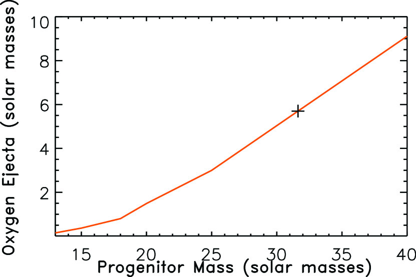
Figure 6: Nomoto et al. 1997 predict specific amounts of oxygen as a function of progenitor mass. The estimated ejecta mass (marked by a cross on the plot) indicates a massive progenitor of $\sim$32 M_⊙, assuming a linear interpolation between the nearest models.

We used the nucleosynthesis models of Nomoto et al. (1997) to relate our estimate of oxygen ejecta mass to the progenitor mass. Oxygen provides a particularly sensitive indicator of progenitor mass, as shown in Figure 6. Our estimate of oxygen ejecta mass suggests a massive progenitor of between Nomoto’s 25 M_⊙ and 40 M_⊙ models. The correlation between ejecta mass and progenitor mass is essentially linear for Nomoto models from 25 M_⊙ to 70 M_⊙. Assuming a linear interpolation between models is appropriate, a progenitor mass of $\sim$32 M_⊙ is indicated.

Hughes (1994) has analyzed ROSAT HRI observations of E0102-72. He found evidence for a ring component and a shell component, much as suggested by the HETG observation. Hughes finds higher densities for the ring component, (n$\sim$6.0 cm^-3, assuming solar abundances) and obtains a mass estimate of up to 75 M_⊙ for the x-ray emitting gas of the SNR (assuming a filling factor of 1.) He concludes that, even for a small filling factor of $\sim$0.1, the progenitor was a massive star.

Blair et al. (2000) examined optical and UV spectra and compared derived ejecta abundances to the models of Nomoto et al. (1997). Their abundance ratios appear to be well approximated by a 25 M_⊙ model. Because they find no significant Fe or Si, they suggest that the progenitor was a W/O star that exploded as a type Ib supernova. Interestingly, they estimate approximately twice as much Ne as predicted by the 25 M_⊙ model. The HETG estimate for the neon ejecta, $\sim$2 M_⊙, is also larger than expected, about three times what would be expected from 25 M_⊙ or 40 M_⊙ Nomoto models.

The HETG results are consistent with Blair et al. (2000) and support the conclusion of a massive progenitor. Several assumptions have a significant impact on our calculations. The most important is the assumption of a “pure metal” plasma. If this assumption is incorrect (and instead hydrogen dominates the plasma composition), the value of n_e will be underestimated by a factor of order $\sim$20. The ejecta mass estimate is smaller by the same factor. This would place the progenitor mass in the range 13–15 M_⊙. Our assumptions about volume, filling factor $\eta$, and oxygen emissivity $\epsilon$ are all less significant, with M_O $\propto$ $\sqrt{\eta V/\epsilon}$. Even accommodating large uncertainties (i.e., a factor of two in volume, $\eta$ as low as 0.1, and a factor of 2.5 variation in $\epsilon$, accounting for the full allowed range in Figure 5), the results do not indicate a progenitor less massive than 20 M_⊙.

Assuming n_e$\sim$0.9 cm^-3, inspection of Figure 5 implies that the ionization age of E0102 is longer than the kinematic age (1000–2000 years). Indeed, if the best-fit $\tau$ ($\sim$25,000 yr cm^-3) is correct, the kinematic age would require n_e = 12–25 cm^-3, although much smaller values are needed (n_e = 1–2 cm^-3) for the lower limit of $\tau$ in the “allowed” range of Figure 5. (For the XSPEC NEI model, the emission-weighted $\tau$ is lower than for the vnpshock model: The best-fit NEI value, $\tau$ $\sim$ 4,500 y cm^-3, would require n_e = 2–5 cm^-3 for an elapsed time of 1000–2000 yr.) Given that our estimate of n_e obtained with a “pure metal” plasma model represents a lower limit, these values are within the range of uncertainties.

4 Ring Diameter and Ionization

The general ring structure of the SNR recurs in each of the images of the individual X-ray lines in Figures 1 and 2, but an important systematic difference is seen in ring diameter. This is evident in the top row of Figure 4, which juxtaposes dispersed lines of helium-like and hydrogen-like oxygen on the same spatial scale for comparison. The helium-like line is clearly emitted by a region of smaller diameter than the hydrogen-like line. A similar effect may be noted for neon (middle row of Figure 4).

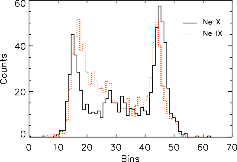
Figure 7: The cross dispersion histograms of the MEG $-1$ orders of helium-like Ne IX and hydrogen-like Ne X lines are overlaid. The difference in the two histograms shows that the emitting regions for the two X-ray lines are different. The H-like Ne X line is generated at larger radius, closer to the site of interaction between the CSM and the ejecta. This suggests the action of the reverse shock.

The top and bottom edges of the bright ring images in the dispersed spectrum were measured by extracting the intensity profiles along a segment perpendicular to the dispersion direction. (The analysis was restricted to perpendicular regions in order to minimize the effects of Doppler shifts, which distort dispersed images along the dispersion direction.) The profiles, or cross-dispersion histograms, for the neon lines of Figure 4 are shown in Figure 7. The cross-dispersion direction is vertical in each image of Figure 4; thus, the left and right peaks of the histogram in Figure 7 respectively trace the intensity profiles through the bright arc of the southeast and the “shelf” to the north. Clearly, the helium-like neon ring is measurably smaller than that of its hydrogen-like counterpart.

An empirical model was used to fit the emission profile and localize the peak of the emission. The model contained the essential elements described in Section 6: an expanding, ring-like shell inclined to the line-of-sight. To better fit the steep peak profile, the radial distribution was given a power law dependence.

The fitted location of the SNR edge along the northern “shelf” is plotted for seven bright X-ray lines (corresponding to n=2 to n=1 transitions) in Figure 8. For each element, the hydrogen-like lines (connected by the top curve) lie outside their corresponding helium-like lines (connected by the bottom curve) by a few arcseconds. This is clearly an ionization effect, unrelated to stratification or segregation of elements, because different ionization stages of the same element are separated.

We attribute the spatial separation of ionization states to changing ionization structure due to passage of the reverse shock through the ejecta. The reverse shock, driven by the retardation of the ejecta as it sweeps up CSM, propagates inward relative to the frame of the (moving) ejecta (McKee, 1974). In this case, the plasma in the outer regions of the ejecta has had a longer time to react to the passage of the reverse shock and has experienced a higher degree of ionization. This was the conclusion reached by Gaetz et al. (2000) based on an X-ray difference map and radial profile analysis of O VII and O VIII emission from direct Chandra ACIS images of E0102. The HETGS spectral images clearly confirm this ionization stage separation for each of the elements.

4.1 Ionization Structure

If the progress of the reverse shock is indeed the controlling mechanism for the spatial segregation of Figure 8, we hypothesize that the location of the SNR edge, (i.e., the peak of the radial emission profile), correlates with the ionization timescale, $\tau$. We apply a simple model, assuming a fixed T_e of 1.14 keV (Sasaki et al., 2001) and the plane parallel vnpshock model (Borkowski et al., 2001) in a uniformly mixed plasma. For each X-ray line, at a fixed temperature the emissivity reaches its peak at a unique value of $\tau$. We assign this value of $\tau$ to the X-ray line, and plot it in Figure 9 against the measured radial distance of the edge (from the SNR center). Measurements are independently plotted for two edges of the SNR: the bright linear “shelf” to the north, and the southeastern arc.

The general trend in Figure 9 shows increasing $\tau$ with increasing radial distance. The radial distribution suggests that the various elements are intermingled, e.g., the bottom curve (corresponding to the northern shelf) in Figure 9 shows lines of O VIII and Mg XI situated between Ne IX and Ne X. The similarity of the emission regions of the three elements of Figure 4 is also compatible with an assumption of substantial blending of the elements. The ionization stages of these elements are interleaved in just the order one would expect from a homogeneous plasma with an inward-propagating shock. The specific values of $\tau$ depend on the assumed temperature in the model, and indeed are selected for maximum emissivity. These are not expected to reflect the actual specific conditions of the SNR plasma, but to illustrate the correlation between radius and ionization timescale: The monotonic trend seen in Figure 9 holds for any temperature over a wide range (i.e., 0.5 to 1.5 keV). Although any workable model must consider additional parameters, this correlation is compatible with an interpretation in which the arcsec differences in ring diameter are attributable to the changing ionization structure resulting from the reverse shock.

5 Image Distortions and Doppler Shifts

Doppler shifts due to center-of-mass bulk motion along the line of sight will produce a systematic shift in the position of all of the dispersed images proportional to wavelength. In contrast, high velocity motions within the remnant (relative to its center of mass) will cause Doppler shifts which distort the dispersed images along the dispersion direction. (No distortions are introduced in the cross-dispersion direction by velocities in the SNR). The magnitude of the observed distortions therefore provides an emission-weighted measure of the velocity structure in the X-ray emitting gas in the remnant.

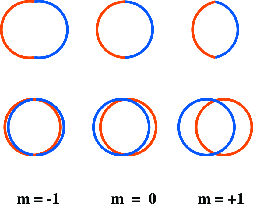
Figure 10: Cartoon illustrating that Doppler shifts distort dispersed order images. The top row (center) depicts a source comprised of a thin circular ring with redshifted eastern half and blueshifted western half. Doppler redshifts in the dispersed images produce dispersion further outward, away from zeroth order, and blueshifts are a little less dispersed, toward the zeroth order at the center. This results in dispersed images which are not circular, as shown by the “stretched” $-1$ order (left) and the “squeezed” +1 order (right). The bottom row illustrates a situation similar to our model for E0102. The center panel schematically illustrates a 3-dimensional source appearing as a thick ring with separated red- and blueshifted components, such as found in Figure 13. (Such an arrangement might be associated with an expanding non-spherical distribution of matter inclined to the line-of-sight.) For simplicity, only the inner and outer edges of the ring are represented. Due to Doppler shifts, the $-1$ order dispersed image (left) shows a narrowed ring, while the +1 order image (ring) shows a broadened ring. This effect is evident in Figure 11. Thus, Doppler shifts result in +1 and $-1$ order images which differ in shape (top row), and effective width (bottom row) of the ring.

Velocity structure can be distinguished from spatial variations in the emissivity by combining information from the two sets of gratings and from the plus and minus dispersion orders. A dispersed image in the light of a single line that is distorted due to intrinsic spatial variations will look identical on either side of the zeroth order (the plus and minus order dispersed images should look the same). A distortion due to a wavelength (Doppler) shift will appear with opposite effects in the plus and minus orders, (i.e., a shift to longer wavelength moves to the right in the plus order but to the left in the minus order image, showing reflectional symmetry about zeroth order), with the constraint that any distortions seen in the MEG data should amplified by a factor of two in the HEG data due to the difference in grating dispersion (with small corrections for the different roll angles of the HEG and MEG dispersions). This is illustrated in Figure 10: A thin ring of emission with red- and blueshifted regions will distort as shown in the top row. A thick ring, as might be represented by an expanding cylinder tilted to the line of sight, would show the effect in the bottom row. The $-1$ order image appears sharper, while the +1 order is broadened.

The impact of velocity structure is clearly evident in the Chandra spectrum, as shown in Figure 11. This figure displays side-by-side the dispersed MEG $-1$ order, the undistorted zeroth order, and the MEG +1 order for Ne X Lyman $\alpha$. Overlaid on these images are alignment rings to assist in identifying distortions. There are clear distortions of the dispersed images relative to the zeroth order. Moreover, the -1 and +1 order Ne X Lyman $\alpha$ images are distinctly different from each other, with a sharper $-1$ order and a blurred or broadened +1 order, analogous to the situation depicted in the bottom row of Figure 10. These characteristics indicate velocity structure within the SNR, and suggest a first approach to modeling this structure. These topics are discussed in the remainder of this section and in Section 6, respectively.

5.1 Analysis

For the analysis of velocity structure, we focused on Ne X Ly $\alpha$ and O VIII Ly $\alpha$ because these lines are bright and their images have minimal contamination from nearby lines. We relied on Obsid 120 alone for most of the analysis, adding Obsid 968 for confirmation. Finally, we used event coordinates given in the tangent-plane coordinate system (i.e., level 1 coordinates) to facilitate direct comparison between dispersed and undispersed images in the same coordinate system.

To quantify the distortions in the dispersed images, we extracted dispersed and undispersed images in such a way that undistorted features would have identical pixel coordinates. This is illustrated in Figure 12. First we selected a reference pixel coordinate at the center of the zeroth order image. We then computed the coordinates of the reference point in the dispersed image using the line wavelength, observation roll angle, and calibrated values of the grating dispersion and tilt angle. We extracted first-order dispersed events centered on this computed position, and formed an image with one axis parallel to the dispersion direction and the other along the cross-dispersion direction. By comparing the images of the dispersed lines with undispersed zeroth-order images filtered closely on the ACIS-S energy of the line, we were able to measure the distortions at various positions along the ring, and assign a corresponding Doppler velocity.

Using this image alignment technique, the pixel coordinates of the extracted images were aligned to within the uncertainty of the grating wavelength scale, corresponding to a velocity uncertainty of $\sim$200 km s^-1. Because the extracted images were accurately aligned using the rest wavelengths of the emission lines, we conclude that the Doppler shift due to motion of the center of mass of E0102 is below our detection limit, indicating that the center-of-mass bulk velocity of the remnant is less than $\sim$200 km s^-1.

5.2 Doppler Shift Statistical Significance

To establish Doppler shifts as the cause of the distortions, we applied the Kolmogorov-Smirnov (KS) test to the event data to investigate the possibility that the apparent distortions might be consistent with Poisson noise. We adapted it to compare event distributions taken from slices in the various images both along the dispersion direction and along the cross-dispersion direction.

A priori, if Doppler shifts are the cause of image distortions, we expect different conclusions from the KS test depending on the the orientation: Doppler shifts affect the dispersion direction, but do not affect the cross-dispersion direction. Using the language of the KS test, we expect that the cross-dispersion slices are being drawn from the same population, but, because of the Doppler distortions, the dispersion-direction slices are not. We conclude that, to high confidence, the observed dispersion-direction distortions are real and are not merely due to statistical fluctuations.

5.3 Centroid Shifts

Having concluded that the distortions are real and attributable to Doppler shifts, the next step is to quantify these distortions in terms of the velocity structure in the SNR. In general, the line of sight samples a distribution of velocities leading to Doppler shifts which would smear the dispersed images in a way that is difficult to quantify in terms of a simple statistic. However, because of the high degree of symmetry in E0102, these Doppler shifts combine somewhat fortuitously to “sharpen” the SE limb of the $-1$ order dispersed images and to shift the centroid of that limb in a way that is consistent with bulk motion of the entire SE limb away from the observer.

Although this localized centroid shift is consistent with bulk motion, the overall structure can be more naturally explained in a model based on radial expansion, similar to that depicted in the bottom row of Figure 10. In this section, we focus on those portions of the remnant where we observe directly measurable Doppler shifts. These cases are of interest because they represent a direct, model-independent detection of motion within the remnant. In Section 5.4 we use a Maximum-Entropy technique in which the dispersed and undispersed images are fitted simultaneously to extract a detailed model of the remnant’s spatial structure and velocity field.

Centroid shifts along the dispersion direction were determined by measuring image centroids within an extraction box, adjusted so that the result was insensitive to the details of the size and position of the box. Confidence limits were estimated through Monte-Carlo trials using subsamples of observed events. Our results for oxygen and neon are summarized in Tables 7 and 8, and discussed in Sections 5.3.1 and 5.3.2, respectively.

Although measurement of the centroid shift has the advantage of being model-independent, it is difficult to apply to regions with complex morphology and reveals only the integrated properties of the region, yielding an emission-weighted mean velocity. For these reasons, the technique is not well suited to portions of the remnant which are smeared in the dispersed image, i.e., the western portion of the $-1$ order. For this reason, Tables 7 and 8 report results only for the eastern side of the SNR, and only a single mean velocity component is obtained in each case.

5.3.1 O VIII Ly $\alpha$

The MEG $-1$ order image for O VIII Ly $\alpha$ allowed a clean measurement for its eastern side, but the western side was blended with a nearby X-ray line, O VII (1s-3p). Although the MEG +1 order is unblended and could provide a cleaner measurement, it had insufficient counts to be useful. Thus, only eastern limb measurements are reported in Table 7. The SE limb of the MEG -1 dispersed O VIII Ly $\alpha$ image shows a large centroid shift relative to the energy-filtered zero-order image. It is consistent with a recession velocity on the order of $\sim$1000 $\pm$ 100 km s^-1, indicating that the material dominating this emission is probably on the back side of the remnant.

Although the zeroth order image is filtered around the energy of the O VIII Lyman $\alpha$ line, it is contaminated with O VII triplet photons. This could affect the reference zeroth order position, with a resultant error in the Doppler shift measurement. Moreover, corroboration of the Doppler shift interpretation using the MEG +1 order image is not possible because the plus order image has insufficient counts. Due to blending and low surface brightness, we were unable to determine whether or not the He-like triplet lines show the same distortion. The large velocities associated with the Doppler shift measurements of the O VIII Lyman $\alpha$ line are comparable with velocities measured for optical knots. These knots generally lie interior to the brightest portions of the X-ray bright ejecta, and also show complex, asymmetric structure (Tuohy & Dopita, 1983).

5.3.2 Ne X Ly $\alpha$

The MEG $-1$ order image of Ne X Ly $\alpha$ had measurable red shifts on the eastern side, but the dispersed images shown in Figure 11 indicate that both red and blueshifts are associated with the western side. Because of the complex morphology of the western side, no unambiguous centroid shifts were apparent and therefore no measurements are reported in Table 8 for the western side of the SNR. The observed centroid shifts in the SE limb of the MEG $-1$ order Ne X Ly$\alpha$ image are significantly smaller than those found for O VIII Ly $\alpha$, partly due to the shorter wavelength. The observed shifts are consistent with a recession velocity of $\sim$ 450 $\pm$ 150 km s^-1 in the SE limb.

5.3.3 Two Velocity Components

The Doppler measurements of the SE limb revealed redshifts, suggesting material on the backside of the remnant. However, because the SE limb of the MEG $-1$ order image is sharper than the +1 order image in both O VIII and Ne X, we can conclude that both receding (red) and approaching (blue) velocity components are present in that region. As shown in Figure 10, this line of sight velocity structure fortuitously “sharpens” the image in the -1 dispersed order but “blurs” the +1 order. Centroid shift measurements are inadequate to describe this situation, where red and blue shifts coexist within the same two-dimensional region of the sky-image. Section 5.4 describes the alternative approach we have taken to map the velocity structure in two dimensions.

5.4 Two Dimensional Spatial/Velocity Analysis

To examine the SNR velocity structure in more detail, we have developed Doppler velocity imaging techniques to extract a three-dimensional, spatial-velocity data cube representation of the source, analogous to narrow-band Fabry-Perot imaging in the optical/UV. We began with a simple model of the SNR with discrete velocity structure, as applied to the Ne X Lyman $\alpha$ line. This source model consisted of a simple data cube with two spatial dimensions and a wavelength dimension. Five wavelengths were selected distributed about the Ne X Lyman $\alpha$ line rest wavelength (12.1322 Å) with Doppler shifts corresponding to velocities -2V, -V, 0, +V, +2V. An additional wavelength of 11.56 Å  was added to account for the rest wavelength of the weaker Ne IX (1s-3p) line whose image intersects the Ne X Ly $\alpha$ image (see Figure 4). The spatial dimension representation was a $34\times 34$ array of square cells, each measuring three ACIS pixels on a side. For each velocity plane, this array of cells traced the Ne X Lyman $\alpha$ emission in the undispersed zeroth order image.

The $34\times 34\times 6$ data cube model was forward-folded to create modeled images of the plus and minus order dispersed data. In an iterative conjugate gradient scheme, the model data cube values were then adjusted to obtain the best fit between the modeled dispersed data and the measured data. The figure of merit for the fitting was the sum of the $\chi^{2}$ measure of model and dispersed data agreement and a negative entropy term measuring the deviation of the zeroth-order image planes from the observed zeroth-order image (i.e., there is a penalty term when the velocity plane deviates from the zeroth order image.) This procedure was carried out with the velocity parameter V set to values between 500 km s^-1 and 1250 km s^-1. The overall best-fit was found for V$\sim$900 km s^-1 and gave modeled MEG +1 and $-1$ order images that were nearly identical to the observed images.

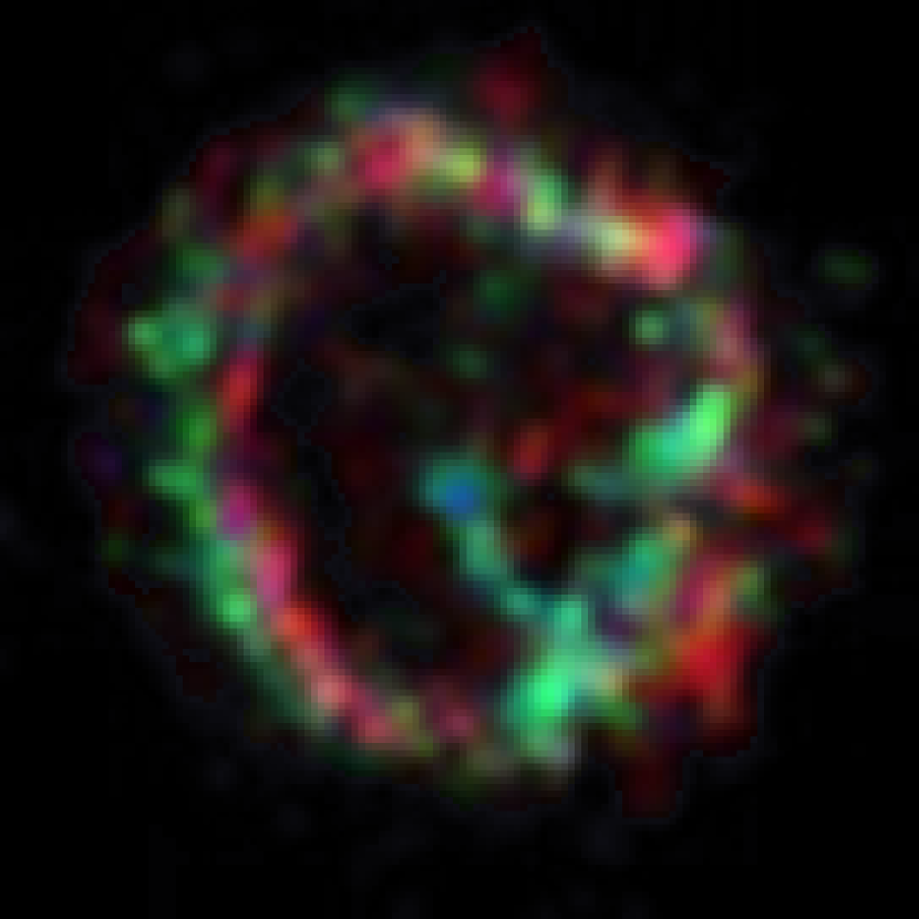
Figure 13: Velocity planes referenced to the zeroth order image are depicted for Ne X Lyman $\alpha$. A single red plane represents the sum of the two redshifted planes +1800 km s^-1 and +900 km s${{}^{-}1}$, green is the -900 km s^-1 blueshifted plane, and blue corresponds to the -1800 km s^-1 blueshifted plane. The zero-velocity plane is not shown, but lies roughly between the red- and blueshifted regions. These three planes, normalized to their maxima, determine the RGB contributions to the color map using the CXC/Ciao tool “dm2img”. Thus, where redshifts and blueshifts coincide, the color representation is yellow. The striking red/blue offset is qualitatively consistent with preliminary modeling, where the emission is concentrated toward an equatorial plane inclined to the line of sight.

The zeroth-order data cube values can be used to create a color-coded velocity image of the Ne X Lyman $\alpha$ emission. In the image of Figure 13, red represents the sum of the two redshifted planes (1800 km s^-1 and 900 km s^-1), which were added because each traced essentially the same spatial region; green represents the $-$900 km s^-1 blueshifted plane, and blue corresponds to the -1800 km s^-1 highly blueshifted plane. The zero-velocity plane is not shown, but lies roughly between the red- and blueshifted regions. This image clearly shows the spatial separation and structure of the red- and blueshifted velocity components in the remnant. This figure is a preliminary result from this new analysis technique and further refinement and error estimation is ongoing.

It is clear from the Figure 13 that both the eastern and western sides of the SNR contain red- and blueshifted components. Along both sides of the SNR, the redshifted regions are situated westward of blueshifted regions, echoing the arrangement depicted in the bottom row of Figure 10. The image suggests spatially offset rings of red- and blueshifted emission, as might occur for a cylindrical or elongated distribution which is viewed off-axis. The placement of the zero velocity emission is consistent with such a model. In particular, the zero-velocity component does not lie outside the red/blue regions, as would be expected for a spherical distribution. Such a simple model invites extending the two-dimensional Doppler map to a three-dimensional physical picture of the SNR, as discussed in the next section.

The “spoke” region in Figure 13 shows a dominance of blue shifts, suggesting that this feature is on the front (near side) of the SNR. Fabry-Perot measurements by Eriksen et al. (2001) also reveal blueshifts among [OIII] filaments measured in that region, with maximum velocities in excess of 2100 km/s. They conclude that this may be a dense clump of shocked material on the front of the remnant, although a component near zero velocity is also detected in the spoke region. The Eriksen et al. (2001) [OIII] measurements also indicate more moderate blueshifts coincident with the SE arc seen in the X-ray. Tuohy & Dopita (1983) present [OIII] images of E0102 which confirm the blueshifts seen in regions of the spoke and the SE arc, and also report a redshifted filament nestled between.

Our velocity plane analysis gives an estimate of the rms velocity dispersion of the Ne X line of $\sim$1100 km s^-1. From the broadening of emission lines observed with the RGS on XMM-Newton, Rasmussen et al. (2001) place a lower limit of 1350 km s^-1 on the expansion velocity of the ejecta assuming a flat velocity profile for an expanding shell. The rms equivalent for this lower limit and profile is 800 km s^-1, in good agreement with our velocity plane analysis.

6 3D Spatial/Velocity Model

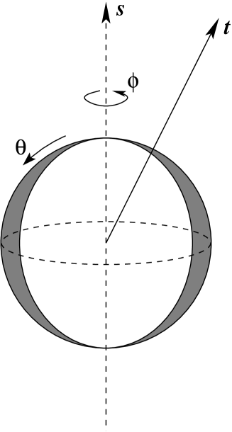
Figure 14: Schematic diagram of axisymmetric model geometry. $\bf s$ is a unit vector along the axis of symmetry. $\bf t$ is a unit vector pointing toward the telescope. The polar coordinate is $\theta$ and azimuthal coordinate is $\phi$. In the preferred model orientation, $\bf t\cdot s=\cos 34\arcdeg$. Viewed from this angle, the matter distribution in projection approximates the observed ellipticity of the zero-order image. The major axis of this ellipse is parallel to the vector $\bf t\times s$, which points $\sim$10^∘ clockwise from North. The emitting material fills a spherical shell with inner radius $\sim$4.3 pc and thickness $\sim$1.2 pc (these are merely representative numbers derived from the zeroth order image). The density distribution within the shell is indicated qualitatively by the thickness of the grey shaded region (see text for details). The emission fills the shell, but is concentrated toward the equatorial plane. This simple model reproduces many of the features of the HETGS spectrum, but does not reproduce the separation of redshifted and blueshifted components seen in Figure 13.

We have constructed a preliminary empirical model of the spatial and velocity structure. Diffuse emission from the interior of the observed ring rules out a purely toroidal geometry, but is much weaker than would be expected from a uniform spherical shell. We infer an intermediate geometry consisting of a non-uniform spherical shell with azimuthal symmetry whose axis is inclined to the line of sight. This is illustrated in Figure 14. We take the inclination to be such that the east side of the SNR is redshifted (i.e., tilted away from the observer) and the west side is blueshifted. The remnant may be intrinsically elliptical, but a viewing asymmetry must nonetheless be present, as indicated by the blurred +1 order and sharp -1 order of Figure 11 and the suggestion of Figure 13. Our empirical model of the emissivity distribution has the form

$$\varepsilon(r,\theta)=\varepsilon_{0}f(r)\exp\left(-\frac{\cos^{2}\theta}{2\sigma^{2}}\right)$$ (4)

where $r$ is the radial coordinate, $\theta$ is the polar angle and where the radial distribution within the shell has the form

$$f(r)=\begin{cases}\left(\frac{r-r_{\rm min}}{r_{\rm max}-r_{\rm min}}\right)^{\alpha}&(r_{\rm min}\leq r<r_{\rm max}),\\ 0&{\rm otherwise}\end{cases}$$ (5)

The Gaussian $\sigma$ is chosen so that 85% of the emission originates within $\pm$30^∘ of the equator. Within the shell, we assume that the ejecta expands with velocity proportional to radius. Interestingly, Hughes (1988) deduced that the surface brightness distribution measured with the Einstein HRI also indicated that the emission was concentrated in a thick ring rather than a spherical shell, although the width of his ring was larger, distributed through an opening half-angle of 67^∘. Hughes (1994) found that ROSAT HRI data required both ring-like and shell-like components.

Our simple 3D model for E0102 reproduces many of the features of the HETGS spectrum. The expansion of the shell and inclination of the symmetry axis to the line of sight effectively reproduce the intriguing difference between the narrow $-1$ order and the broadened +1 order seen in the dispersed images of Ne X Lyman $\alpha$ in Figure 11. Moreover, inclining the model ejecta ring to the line of sight results in enhanced emission due to projection effects (i.e. limb brightening), and may partially account for the enhanced emission in the vicinity of the northern “shelf” and the bright southeastern arc. Finally, the elements of this model provide a good representation for the edge profiles. However, this simple model falls short in several respects. It does not correctly reproduce the elliptical shape of the zeroth order image, and neglects individual features such as the radial “spoke”. More importantly, this model does not reproduce the striking separation of blueshifted and redshifted components seen in Figure 13 and depicted for the m=0 order in the bottom row of Figure 10.

Other 3D models are being considered to describe the spatial and velocity structure of the SNR. A cylindrical or elongated (e.g. barrel-shaped) distribution is an inviting candidate as it will make a better match with the Doppler map of Figure 13. In such a case, the ring thickness seen in Figure 3 would be interpreted as the projection of a much thinner region extending in three-dimensions and inclined to the line of sight. Such a model must simultaneously satisfy the edge profiles and other constraints. The second GTO observation of E0102 taken in December, 2002, will help resolve these questions. It was carried out at a different roll angle, and therefore provides complementary Doppler information to the first observations. The two sets of GTO observations, taken together, will be used to refine the model. Although the simple candidate 3D models we have described are incomplete, they will serve as a point of departure for future work.

7 Discussion

Our Doppler analysis of E0102 indicates velocities of order $\sim$1000 km s^-1 and a toroidal (or possibly cylindrical) distribution. Several other oxygen-rich SNRs show evidence for a ring-like geometry with expansion velocities $\sim$2000 km s^-1. X-ray observations of Cas A by Markert et al. (1983) using the Focal Plane Crystal Spectrometer on the Einstein Observatory revealed evidence for asymmetric Doppler shifts which they interpreted as a ring of material with an expansion velocity in excess of 2000 km s^-1. ( Hwang et al. (2001) consider a highly asymmetric explosion and subsequent evolution to account for their Chandra Doppler map of Cas A.) X-ray observations of G292.0+1.8 by Tuohy et al. (1982) revealed a bar-like feature which they attributed to a ring of oxygen-rich material ejected into the equatorial plane. Examination of a velocity map generated from optical observations of E0102-72 led Tuohy & Dopita (1983) to suggest that its velocity structure could be modeled in terms of a severely distorted ring of ejecta. Lasker (1980) also found toroidal expansion in the optical lines of N132D.

A cylindrical or toroidal distribution of ejecta can arise as a result of the core collapse process or through the interaction of the CSM. Khokhlov et al. (1999) discusses evidence that the core collapse process is asymmetric. Spectra of core collapse supernovae are polarized, indicating an asymmetric distribution of ejected matter (Wang et al., 2001). Neutron stars are formed with high space velocities (Strom et al., 1995) and “bullets” of ejecta penetrate remnant boundaries (Fesen & Gunderson, 1996; Taylor et al., 1993). Simulations of jet-induced core collapse supernova explosions (Khokhlov et al., 1999) result in high velocity polar jets and a slower, oblate distribution of ejecta. Two dimensional models of standing accretion shocks in core collapse supernovae (Blondin et al., 2003) are unstable to small perturbations to a spherical shock front and result in a bipolar accretion shock, followed by an expanding aspherical blast wave.

Asymmetry in the supernova remnant can also be imparted through the influence of the CSM. Blondin et al. (1996) find that SNR show evidence of being “relics of supernovae interacting with non spherically symmetric surroundings.” Igumenshchev et al. (1992) find aspherical cylindrical symmetry in $\sim$30% of remnants observed with Einstein (Seward, 1990). One of the explanations they propose is that the SNe explode in a medium with a disk-like density distribution determined by the stellar wind from the precursor red supergiant. This density distribution is believed to be heavily concentrated in the equatorial plane. This produces a remnant elongated along the polar axis and having lower density in that direction. Such CSM density distributions from red giant and red supergiants are expected to be common, as evidenced by the case of planetary nebulae (PN). Zuckerman & Aller (1986) found in a sample of 108 planetary nebulae, about 50% were bipolar. PN shapes are currently modeled by a fast wind from a central star colliding with a cylindrically symmetric stellar wind from the precursor red giant (Kwok et al., 1978; Kahn & West, 1985); where mass-loss is enhanced towards the equator, elongation along the poles results. Blondin et al. (1996) have studied interactions of supernovae with an axisymmetric CSM and find that the asymmetry generally follows the asymmetry of the CSM (Blondin, 2001), but for a sufficient angular density gradient, it is possible to obtain protrusions or jet-like structures along the axis. Thus, the asymmetric structures inferred from our data, whether emission dominated by an equatorial ring, or an elongated cylindrical-type structure, are compatible with current models of SNe explosions and subsequent interactions with the CSM.

The ionization structure of the SNR as revealed in Figure 9 provides a compelling picture of the action of the reverse shock. For two different interaction sites in the SNR (the northern “shelf” and the SE arc), up to seven different X-ray lines follow a pattern that can be simply explained by a time-dependent ionization in a uniform abundance plasma. There appears to be substantial mixing of the elements, as indicated by the remarkable similarity of the O, Ne and Mg rings shown in Figure 4, and the intermingling of peak emission regions for lines of oxygen, neon and magnesium as shown in Figure 9.

8 Summary

The HETGS spectrum of E0102 yields monochromatic images of the SNR in X-ray lines of hydrogen-like and helium-like oxygen, neon, magnesium and silicon with little iron. Plasma diagnostics using O VII and O VIII lines summmed over the entire remnant confirm that that the SNR is an ionizing plasma in the low density limit, and give a best-fit oxygen plasma model represented by a plane-parallel shock (vnpshock) of electron temperature $T_{e}$ = 0.34 keV and ionization timescale log $\tau$ $\sim$11.9 s cm^-3. Assuming a pure metal plasma, the derived oxygen ejecta mass is $\sim$6 M_⊙, consistent with a massive progenitor.

The dispersed X-ray images reveal a systematic variation of ring diameter with ionization state for all elements. We find that this structure is consistent with the evolution of the ejecta’s plasma after passage of the reverse shock, and cannot be explained by radial stratification of the elements. Future work will include a second observation and focus on the ionization structure and emission distribution in the northern linear “shelf” feature, and across the bright southeastern arc.

Distortions within the dispersed images reveal Doppler shifts due to bulk motion within the remnant. Measurements for lines of neon and oxygen indicate velocities on the order of 1000 km s^-1, consistent with velocities measured for optical filaments. A two-dimensional spatial/velocity map has been constructed which shows a striking spatial separation of redshifted and blueshifted regions.

A simple three-dimensional physical model of the SNR shows rough agreement with many of the features attributed to Doppler shifts. This 3D model consists of a nonuniform spherical shell with azimuthal symmetry, and with emission concentrated toward the equatorial plane. The symmetry axis is inclined with respect to the line-of-sight, and the shell is expanding. We find that this model reproduces some, but not all, of the essential features of the HETGS spectrum. Cylindrical distributions for the reverse-shocked ejecta plus a blastwave component will be another candidate model for future investigation. The asymmetric structures implied by the data are compatible with current models of SNe explosions and subsequent interactions with the CSM.

Table 1: HETG Observations of 1E0102.2-7219

	Obsid 120	Obsid 968
nominal observation time	90 ksec	48.6 ksec
roll angle (degrees)	12.0088	11.1762
effective observation time	86.9 ksec	48.6 ksec
date observed	Sept 28, 1999	October 8, 1999
zeroth order	55.3	29.5
MEG $\pm$ 1 order	45.8	25.5
HEG $\pm$ 1 order	15.0	7.9

Table 2: Observed Flux

X-Ray line	Energy	$\lambda$	flux	error	correction	continuum	net flux	net error
	(keV)	(   $\AA)$		(1$\sigma$)	factor
O VII Forbidden	0.5610	22.10	13.95	2.17	1.024	.92	13.03	2.18
O VII Resonance	0.5740	21.60	24.38	3.80	1.027	.96	23.42	3.80
O VII Triplet	0.5675	21.85	49.63	1.54	1.027	2.54	47.09	1.62
O VIII Lyman $\alpha$	0.6536	18.97	37.31	8.45	1.020	1.22	36.09	8.45
O VII 1s–3p	0.6655	18.63	6.23	1.31	1.040	1.29	4.94	1.34
O VII 1s–4p	0.6977	17.77	2.97	.41	1.049	1.22	1.75	0.48
Fe XVII NeVIII	0.7270	17.05	2.89	.40	1.048	1.44	1.45	0.49
O VIII Lyman $\beta$	0.7744	16.01	6.37	.67	1.079	1.28	5.09	0.72
O VIII Lyman $\gamma$	0.8168	15.18	3.75	.39	1.092	1.32	2.43	0.66
Ne IX Forbidden	0.9050	13.70	7.14	1.24	1.097
Ne IX (Res + Intercomb)	0.9225	13.49	13.49	1.41	1.073
Ne IX Triplet	0.9137	13.57	23.18	1.28	1.092
Ne X Lyman $\alpha$	1.0221	12.13	9.72	.66	1.048
Ne IX 1s–3p	1.0725	11.56	3.09	.24	1.046
Ne IX 1s–4p	1.1271	11.00	1.99	.39	1.045
Ne X Lyman $\beta$	1.2108	10.24	2.07	.31	1.037
Mg XI Triplet	1.3521	9.17	3.77	.27	1.024
Mg XII Lyman $\alpha$	1.4725	8.42	1.01	.14	1.028
Si XIII Triplet	1.8644	6.65	1.06	.20	1.037

Table 3: Oxygen Line Ratios

Lines	Ratio	error	Ratio	error	90% contours
		(1$\sigma$)		(1$\sigma$)
O VIII Lyman $\alpha$ / O VII Resonance	1.54	.44	1.26	.36	.67 – 1.85
O VII Forbidden / OVII Resonance	.56	.13	.58	.14	.35 – .81
O VIII Lyman $\beta$ / O VIII Lyman $\alpha$	.14	.04	.12	.03	.07 – .18
O VIII Lyman $\gamma$ / O VIII Lyman $\beta$	.48	.15	.46	.14	.23 – .69
O VII 1s–3p / O VII Resonance	.21	.07	.17	.05	.08 – .26
O VII 1s–4p / O VII 1s–3p	.35	.14	.34	.13	.13 – .55

Table 4: O VII Triplet Fitted Line Fluxes

Line	Wavelength	Flux	error	Flux	error
O VII Resonance	21.6015	24.513	4.903	47.871	9.574
O VII Intercombination	20.8036	2.844	0.570	5.647	1.129
O VII Forbidden	22.0977	11.145	2.229	22.741	4.548

Table 5: O VII Triplet Fitted Diagnostic Line Ratios

Diagnostic	Ratio	error	Ratio	error	XMM–Newton	error
		(1$\sigma$)		(1$\sigma$)
R = f/i	3.9	1.1	4.0	1.1	3.4	0.6
G = (i+f)/r	0.57	0.15	0.59	0.15	0.55	0.03
f/r	0.45	0.13	0.48	0.13

Table 6: Assumed Plasma Parameters and Estimated Ejecta Masses

Element	$T_{e}$	log $\tau$	Plasma Model Basis	Ejecta Mass
	(keV)	(s cm-3)		(M⊙)
Oxygen	0.34	11.9	HETG plasma diagnostics	5.7
Neon	0.58	11.9	HETG plasma diagnostics	2.2
Magnesium	0.5	12.0	Hayashi et al. (1994)
Silicon	0.6	11.80	Hayashi et al. (1994)
Iron	3.25	10.45	Hayashi et al. (1994)

Table 7: Eastern Limb, O VIII Ly$\alpha$

Cross-Disp. Slice	Centroid Shift	Velocity
( 20, 30)	$10\pm 4$	$1800\pm 700$
( 10, 20)	$3.2\pm 0.7$	$560\pm 120$
( 0, 10)	$3.0\pm 0.5$	$530\pm 80$
(-10, 0)	$3.8\pm 0.6$	$660\pm 100$
(-20,-10)	$6.2\pm 0.4$	$1100\pm 70$
(-30,-20)	$3.1\pm 0.8$	$550\pm 140$

Table 8: Eastern Limb, Ne X Ly$\alpha$

Cross-Disp. Slice	Centroid Shift	Velocity
( 20, 30)	$2.0\pm 1.4$	$540\pm 390$
( 10, 20)	$3.0\pm 0.3$	$800\pm 80$
( 0, 10)	$0.4\pm 0.5$	$100\pm 150$
(-10, 0)	$1.7\pm 1.0$	$470\pm 280$
(-20, -10)	$1.6\pm 0.4$	$440\pm 100$
(-30, -20)	$1.3\pm 0.5$	$350\pm 140$

Figure 1: Dispersed high resolution spectrum of 1E 0102-7219. Shown here is a portion of the Medium Energy Grating (MEG) -1 order, color coded to suggest the ACIS energy resolution. At right in the figure (with different intensity scaling) is the zeroth order, which combines all energies in an undispersed image. Images formed in the light of strong X-ray emission lines are labeled. The dispersed spectrum is truncated; the resonance line of Si XIII is not shown in the figure.

Figure 2: Dispersed high resolution spectrum of 1E 0102-7219 from MEG $-1$ order, emphasizing faint X-ray lines. The image is summed from the two observation intervals, Obsid 120 and Obsid 968. Transitions from upper levels for various elements and ionization species are indicated. The expected locations of normally bright Fe XVII lines are indicated; Fe is obviously weak in the spectrum. Detector artifacts, such as the chip gaps appearing near O VIII Lyman $\beta$ and midway between O VIII Lyman $\delta$ and Ne IX forbidden, have not been removed. Silicon and faint magnesium transitions are not marked.

Figure 3: Undispersed zeroth order image of 1E 0102-7219, with 2-pixel smoothing. All energies have been included. In addition to the obvious shell structure, note the bright “shelf”-like feature at top, the bright southeastern arc, and the radial “spoke” extending from a knot in the southwest section of the ring. The boundary of the blast wave is also evident in the figure.

Figure 4: The MEG -1 order dispersed images formed by lines of oxygen (top), neon (middle) and magnesium (bottom), shown in dispersion coordinates (rotated $\sim$17^∘ with respect to the orientation in Figure 3). For each element, the helium-like n = 2 to n = 1 triplet is shown at left, and the hydrogen-like n =2  to n = 1 Lyman $\alpha$ line is shown at right. In each case, the forbidden line on the left of the triplet is bright and easily distinguished from the resonance line on the right of the triplet. The intercombination line, located between, is very faint. The faint ring to the right of Ne X Lyman $\alpha$ is Ne IX (1s–3p). Note the disparity of ring size in the top row; distortions of ring shape for Ne X Lyman $\alpha$ in the middle row; and absence of a complete ring in the southern portion of the hydrogen-like stage of magnesium (bottom row). These are taken to be indicators of the passage of the reverse shock, bulk matter Doppler shifts, and inhomogeneous plasma conditions, respectively.

Figure 8: Measured radial distance of the northern edge of the SNR (along the “shelf”) corresponding to the brightest X-ray lines of 1E 0102.2-7219. The hydrogen-like lines (upper curve) lie outside their helium-like counterparts (lower curve) for each element. Error bars on distance are dominated by the quality of the model fit which determines edge location.

Figure 9: The ionization timescale ($\tau$) for which each X-ray line exhibits maximum emissivity is plotted against the measured radial distance, for two regions of the SNR: the linear “shelf” feature to the north, and the bright arc in the southeast. A single constant electron temperature of 1.14 keV has been assumed (Sasaki, et al. 2001). This plot is not expected to reflect the actual specific conditions of the SNR plasma, but to illustrate the correlation between ionization and radius. The plot is consistent with an interpretation of progressive ionization structure due to passage of the reverse shock through the ejecta. Error bars on distance are dominated by the quality of the model fit which determines edge location. Error bars on $\tau$ are set equal to the grid spacing chosen for the plane parallel shock model, vnpshock, and $\tau$ represents $\tau=\tau_{\rm upper}$.

Figure 12: Illustration showing how dispersed and undispersed images are obtained in such a way that undistorted features have identical pixel coordinates. A reference pixel (X) is selected at the center of the zeroth order image and a rectangular extraction region of the desired size is centered on this reference pixel. For the wavelength of interest, the dispersed coordinates of the reference pixel are computed, establishing the location of corresponding extraction region for the dispersed image. First-order events are extracted and images are formed with one axis parallel to the dispersion direction and the other axis along the cross-dispersion direction.

References

- Arnaud (1996) Arnaud, K.A. 1996, in ASP Conf. Ser. 101, Astronomical Data Analysis Software and Systems V, ed. G. Jacoby and J. Barnes (San Francisco: ASP), 17
- Bar-Shalom et al. (1988) Bar-Shalom, A., Klapisch, M. and Oreg, J. 1988, Phys. Rev. A, 38, 1773
- Blair et al. (1989) Blair, W.P., Raymond, J.C., Danziger, J. and Matteucci, F. 1989, ApJ, 338, 812
- Blair et al. (2000) Blair, W.P., Morse, J.A., Raymond, J.C., Kirshner, R.P., Hughes, J.P., Dopita, M.A., Sutherland, R.S., Long, K.S. and Winkler, P.F. 2000, ApJ, 537, 667
- Blondin et al. (1993) Blondin, J.M. & Lundqvist, P. 1993, ApJ, 405, 337
- Blondin et al. (1996) Blondin, J.M., Lundqvist, P. & Chevalier, R.A. 1996, ApJ, 472, 257
- Blondin (2001) Blondin, J.M. 2001, in AIP Conf. Proc. 565, Young Supernova Remnants: Eleventh Astrophysics Conference, College Park, Maryland 2000, ed. S.S. Holt and U. Hwang (Melville: AIP), 59
- Blondin et al. (2003) Blondin, J.M., Mezzacappa, A. & DeMarino, C. 2003, ApJ, 584, 971
- Borkowski et al. (2001) Borkowski, K.J., Lyerly, W.J. and Reynolds, S.P. 2001, ApJ, 548, 820
- Burke et al. (1997) Burke, B.E., Gregory, J.A., Bautz, M.W., Prigozhin, G.Y., Kissel, S.E., Kosicki, B.B., Loomis, A.H., and Young, D.J. 1997, IEEE Trans. on Electron Devices, 44, 1633
- Canizares et al. (2000) Canizares, C.R., Huenemoerder, D.P., Davis, D.S., Dewey, D., Flanagan, K.A., Houck, J., Markert, T.H., Marshall, H.L., Schattenburg, M.L., Schulz, N.S., Wise, M., Drake, J.J. and Brickhouse, N.S. 2000, ApJ, 539, L41
- Canizares et al. (2001) Canizares, C.R., Flanagan, K.A., Davis, D.S., Dewey, D., & Houck, J.C. 2001, in ASP Conf. Proc. 234, X-ray Astronomy 2000, ed. R. Giacconi, S. Serio, & L. Stella (San Francisco: ASP), 173
- Canizares et al. (2003) Canizares, C.R., et al. 2003, in preparation.
-
Chandra Proposers’ Observatory Guide (2002)
Chandra Proposers’ Observatory Guide, Version 5.0, 2002,
http://cxc.harvard.edu/proposer/POG/index.html - Davis et al. (2001) Davis, D.S., Flanagan, K.A., Houck, J.C., Allen, G.E., Schulz, N.S., Dewey, D., and Schattenburg, M.L., 2001, in AIP Conf. Proc. 565, Young Supernova Remnants: Eleventh Astrophysics Conference, College Park, Maryland 2000, ed. S.S. Holt and U. Hwang (Melville: AIP), 230
- Dopita et al. (1981) Dopita, M.A., Tuohy, I.R. and Mathewson, D.S. 1981, ApJ, 248, L105
- Eriksen et al. (2001) Eriksen, K.A. et al. 2001, in AIP Conf. Proc. 565, Young Supernova Remnants: Eleventh Astrophysics Conference, College Park, Maryland 2000, ed. S.S. Holt and U. Hwang (Melville: AIP), 193
- Fesen & Gunderson (1996) Fesen, R.A. & Gunderson, K.S. 1996, ApJ, 470, 967
- Flanagan et al. (2001) Flanagan, K.A., Canizares, C.R., Davis, D.S., Houck, J.C., Markert, T.H., and Schattenburg, M.L. 2001, in AIP Conf. Proc. 565, Young Supernova Remnants: Eleventh Astrophysics Conference, College Park, Maryland 2000, ed. S.S. Holt and U. Hwang (Melville: AIP), 226
- Flanagan et al. (2003) Flanagan, K.A., Canizares, C.R., Dewey, D., Fredericks, A., Houck, J.C., Lee, J.C., Marshall, H.L. & Schattenburg, M.L. 2003, in Proc. SPIE, Vol. 4851, X-Ray and Gamma Ray Telescopes and Instruments for Astronomy, ed. J.E. Trumper, & H.D. Tananbaum (Bellingham: SPIE), 45
- Gaetz et al. (2000) Gaetz, T.J., Butt, Y.M., Edgar, R.J., Eriksen, K.A., Plucinsky, P.P., Schlegel, E.M. and Smith, R.K. 2000, ApJ, 534, L47
- Garmire et al. (2003) Garmire, G.P., Bautz, M.W., Ford, P.G., Nousek, J.A., & Ricker, G.R. 2003, in Proc. SPIE, Vol. 4851, X-Ray and Gamma Ray Telescopes and Instruments for Astronomy, ed. J.E. Trumper, & H.D. Tananbaum (Bellingham: SPIE), 28
- Hayashi et al. (1994) Hayashi, I., Koyama, K., Masanobu, O., Miyata, E., Tsunemi, H., Hughes, J.P. and Petre, R. 1994, PASJ, 46, L121
- Houck & DeNicola (2000) Houck, J.C. and DeNicola, L.A. 2000, in Astronomical Data Analysis Software and Systems IX (ASP Conference Series vol 216: San Francisco), eds. N. Manset, C. Veillet and D. Crabtree, 591
- Hughes & Helfand (1985) Hughes, J.P. and Helfand, D.J. 1985, ApJ, 291, 544
- Hughes (1988) Hughes, J.P. 1988, in Supernova Remnants and the Interstellar Medium, ed. R.S. Roger and T.L. Landecker (Cambridge: Cambridge Univ. Press), 125
- Hughes (1994) Hughes, J.P. 1994, in AIP Conf. Proc. 313, The Soft X-Ray Cosmos: Proceedings of the ROSAT Science Symposium in College Park, Maryland Nov. 8-10, 1993, ed. E.M. Schlegel and R. Petre (New York: AIP), 144
- Hughes et al. (2000a) Hughes, J.P., Rakowski, C.E. Burrows, D.N. & Slane, P.O. 2000a, ApJ, 528, L109
- Hughes et al. (2000b) Hughes, J.P., Rakowski, C.E. and Decourchelle, A. 2000b, ApJ, 543, L61
- Hwang et al. (2001) Hwang, U., Szymkowiak, A.E., Petre, R., and Holt, S.S. 2001, ApJ, 560, L175
- Igumenshchev et al. (1992) Igumenshchev, I.V., Tutukov, A.V. & Shustov, B.M. 1992, Sov. Astron 36(3), 241
- Kahn & West (1985) Kahn, F.D. & West, K.A. 1985, MNRAS, 212, 837
- Khokhlov et al. (1999) Khokhlov, A.M., Hoflich, P.A., Oran, E.S., Wheeler, J.C., Wang, L. & Chtchelkanova, A.Y. 1999, ApJ, 524, L107
- Klapisch et al. (1977) Klapisch, M., Schwab, J.L., Fraenkel, J.S. and Oreg, J. 1977, J. Opt. Soc. Am., 61, 148
- Kwok et al. (1978) Kwok, S., Purton, C.R. & FitzGerald, P.M. 1978, ApJ, 219, L125
- Lasker (1980) Lasker, B.M., 1980, ApJ, 237, 765
- Markert et al. (1983) Markert, T.H., Canizares, C.R., Clark, G.W. and Winkler, P.F. 1983, ApJ, 268, 134
- Markert et al. (1994) Markert, T.H., Canizares, C.R., Dewey, D., McGuirk, M., Pak, C., and Schattenburg, M.L. 1994, in Proc. SPIE2280, EUV, X-Ray, and Gamma-Ray Instrumentation for Astronomy V, ed. O.H.W. Siegmund and J.V. Vallerga (Bellingham: SPIE), 168
- McKee (1974) McKee, C.F. 1974, ApJ, 188, 335
- McNamara & Feltz (1980) McNamara, D.H., & Feltz, K.A. 1980, PASP, 92, 587
- Nomoto et al. (1997) Nomoto, K., Hashimoto, M., Tsujimoto, T., Thielemann, F.-K.,Kishimito, N., Kubo, Y. and Nakasato, N. 1997, Nuclear Physics A, 616, 79
- Plucinsky et al. (2001) Plucinsky, P.P., Edgar, R.J., Virani, S.N., Townsley, L.K., and Broos, P.S. 2001, in ASP Conf. Ser., The High Energy Universe at Sharp Focus, ed. E. Schlegel and S. Vrtilek (St. Paul: ASP),
- Pradhan (1982) Pradhan, A.K. 1982, ApJ, 263, 477
- Rasmussen et al. (2001) Rasmussen, A.P., Behar, E., Kahn, S.M., den Herder, J.W. and van der Heyden, K. 2001, A&A, 365, L231
- Sasaki et al. (2001) Sasaki, M., Stadlbauer, T.F.X., Haberl, F., Filipovic, M.D. and Bennie, P.J. 2001, A&A, 365, L237
- Seward (1990) Seward, F.D. 1990, ApJS73, 781
- Smith et al. (2001) Smith, R.K., Brickhouse, N.S., Liedahl, D.A., and Raymond, J.C. 2001, ApJ, 556, L91
- Strom et al. (1995) Strom, R., Johnston, H.M., Verbunt, F. & Aschenbach, B. 1995, Nature, 373, 590
- Taylor et al. (1993) Taylor, J.H., Manchester, R.N. & Lyne, A.G. 1993, ApJS, 88, 529
- Tuohy et al. (1982) Tuohy, I.R., Clark, D.H. and Burton, W.M. 1982, ApJ, 260, L65
- Tuohy & Dopita (1983) Tuohy, I.R. and Dopita, M.A. 1983, ApJ, 268, L11
- Wang et al. (2001) Wang, L., Howell, A.D., Hoflich, P. & Wheeler, J.C. 2001, ApJ, 550, 1030 (2001)
- Zuckerman & Aller (1986) Zuckerman, B. & Aller, L.A. 1986, ApJ, 301, 772