GRB Redshift Evolution Within the Unified Jet Model

Abstract

HETE-2 has provided new evidence that gamma-ray bursts may evolve with redshift (graziani2003, ). We investigate the consequences of this possibility for the unified jet model of XRFs and GRBs (lamb2003, ). We find that burst evolution with redshift can be naturally explained within the unified jet model, and the resulting model provides excellent agreement with existing HETE-2 and BeppoSAX data sets. In addition, this evolution model produces reasonable fits to the BATSE peak photon number flux distribution – something that cannot be easily done without redshift evolution.

1 Introduction

Most objects at cosmological distances (stars, galaxies, AGN) display evolution of their observable properties with redshift. Since gamma-ray bursts (GRBs) are thought to originate in the core-collapse of massive stars and are observed over a wide range in redshift, it is reasonable to suppose that they might also evolve.

Since the advent of rapid GRB localizations with BeppoSAX and HETE-2, and the consequent follow-up observations, over $30$ GRBs have reported redshift measurements. Using 9 BeppoSAX bursts from amati2002 , plus an additional 11 bursts localized with HETE-2, graziani2003 have been able to strengthen earlier indications that GRBs are brighter at higher redshifts.

A uniform-jet model proposed by lamb2003 has been shown to provide a unified picture of GRBs and XRFs. Considering all bursts to have a “standard energy” but a range of jet opening solid-angles that spans five orders of magnitude, this unified jet model can account for the full range of observed burst properties seen by HETE-2 . Here we extend this unified jet model to account for redshift evolution and show that it can also explain the observed properties of BATSE bursts.

2 Observations of GRB Evolution

Analysis of the BATSE catalog has revealed evidence that GRBs may evolve strongly with redshift. The use of redshift estimators based on burst variability has provided evidence that bursts are intrinsically brighter at larger redshifts than at smaller lloyd2002 ; reichart2001b . Analyzing a set of 9 GRBs with spectroscopically determined redshifts observed by the BeppoSAX satellite, amati2002 also claim evidence for an increase in the isotropic-equivalent energy ($E_{\rm iso}$) with redshift, but they did not include a discussion of possible threshold selection effects.

Recent results from HETE-2 strengthen the evidence for this relationship. Figure 2 from graziani2003 shows the isotropic-equivalent energies $E_{\rm iso}$ and luminosities $L_{\rm iso}$ as a function of redshift for the HETE-2 and BeppoSAX events. After correcting for threshold effects, graziani2003 find that $E_{\rm iso}$ is correlated with redshift at the $5.1$% confidence level, and $L_{\rm iso}$ is correlated with redshift at the $0.9$% confidence level. The observed relationship goes roughly as $E_{\rm iso}\sim(1+z)^{3}$.

3 Unified Jet Model Simulations

The unified jet model of GRBs and XRFs lamb2003 provides a natural explanation for redshift evolution in GRBs. Namely, each burst exhibits a “standard energy” frail2001 ; bloom2003 , but the possible range of jet opening angles varies from fairly large values at low redshift, to very small values at high redshift, according to the relationship given above. That is, evolution in $E_{\rm iso}$ is explained by an evolution of the jet opening solid-angle, $\Omega_{\rm jet}$.

Figure 1: Left: Cumulative distribution of $E_{\gamma}$ values reported by bloom2003 , shown with the best-fit Gaussian. Right: Displacement of $E_{\gamma}$ values from the best-fit central value as a function of redshift. From lamb2003 .

The burst simulations that we have implmented to test the unified jet model also provide a powerful way to explore models including burst evolution with redshift. For each burst, we obtain: (1) A redshift z by drawing from a model of the star-formation rate rr2001 , and (2) a jet-opening solid angle $\Omega_{\rm jet}$ by drawing from specific distribution range in $\Omega_{\rm jet}$ that is fixed at $z=0$ and shifts to smaller values at higher redshifts. We also introduce three Gaussian smearing functions to generate: (1) A spread in jet energy ($E_{\gamma}$, see Figure 1), (2) a spread in $E_{\rm peak}$ around the $E_{\rm iso}$-$E_{\rm peak}$ relation, and (3) a spread in the timescale T that converts fluence to flux. Using these five quantities, we calculate various rest-frame quantities ($E_{\rm iso}$, $E_{\rm peak}$, etc.), and finally, we construct a Band function for each burst and transform it to the observer frame, which allows us to calculate fluences and peak fluxes and determine if the burst would be detected by various instruments (see Figure 2a).

To obtain the model presented here, we sought to roughly match the observed distribution in the ($1+z$, $E_{\rm iso}$)-plane (compare Figure 2b with Figure 2 of graziani2003 ), which displays a range in $E_{\rm iso}$ of $3\times 10^{49}$ to $1.5\times 10^{52}$ ergs at $z=0$ and $6.4\times 10^{51}$ to $3.2\times 10^{54}$ ergs at $z=5$. Assuming the faintest burst at $z=0$ corresponds to $\Omega_{\rm jet}=2\pi$, this translates into a range of $\Omega_{\rm jet}$ of $2\pi$ to $0.0125$ steradians at $z=0$ and $0.0291$ to $5.79\times 10^{-5}$ steradians at $z=5$.

The observed values of $E_{\gamma}$ are taken from bloom2003 , and their distribution is well-fit by narrow Gaussian frail2001 ; bloom2003 ; lamb2003b (see Figure 1a). Figure 1b plots the displacement of these values from the central value as a function of redshift and shows no evidence for evolution of $E_{\gamma}$ with redshift lamb2003 . This rules out the possibility that redshift evolution might be explained by an evolution of the “standard energy”.

Since it relies on the random distribution of burst jet axes with respect to the viewing angle, the universal structured-jet model cannot easily accommodate redshift evolution. The only solution would be for the “jet energy”, $E_{\gamma}$, to evolve with redshift, but that would make it difficult to explain Figure 1 and the results of frail2001 ; bloom2003 .

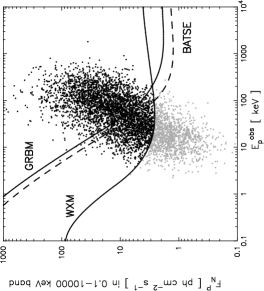
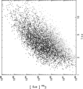
Figure 2: Left: Distribution of bursts in the ($E_{\rm peak}^{\rm obs}$, $F_{\rm N}^{\rm P}$)-plane, showing the threshold curves we use to determine if a burst is detected by various instruments. Black points are bursts detected by the WXM, while gray points are not detected. Right: Distribution of bursts in the ($1+z$, $E_{\rm iso}$)-plane for our best uniform jet with redshift evolution model.

4 Results

Figure 4 compares the cumulative distributions of four observable burst quantities against several possible models. We find that the uniform jet model with burst evolution can adequately describe the observed distributions of localized bursts.

In addition, adding evolution to the uniform jet model replicates the observed distribution of peak photon number fluxes as observed by BATSE. Models without redshift evolution (Figure 3a, dotted curve) tend to overpredict the number of high peak flux bursts. However, models with strong evolution (solid curve) provide excellent agreement with the BATSE distribution. Figure 3b shows the differential distribution of redshifts (for bursts detected by WXM) for the models with and without redshift evolution.

This model makes several predictions. Most observed XRFs are predicted to be at $z<1$. Bursts at low $z$ have $\Omega_{\rm jet}>10^{-2}$ or $\theta_{\rm jet}\sim$ a few degrees. We require a value of the “standard energy” to be $E_{\gamma}\sim 5\times 10^{49}$ ergs, or about $50$ times less than the value reported by bloom2003 . Thus, the fraction of Type Ic supernovae producing GRBs increases from $\sim 0.1$% at $z=0$ to $\sim 10$% at $z\sim 5$. Finally, $70$% of bursts with $z>5$ are detected by the WXM.

Figure 3: Left: Comparison of uniform jet models with redshift evolution (solid) and without (dotted) with the BATSE peak photon number flux cumulative distribution. Right: Predicted observed distribution of redshifts for the uniform jet model with redshift evolution (solid) and without (dotted).

Figure 4: Comparisons of different models with the observed cumulative distributions for $E_{\rm iso}$ (upper left), $E_{\rm peak}$ (upper right), $S_{\rm E}(2-400\;{\rm keV})$ (lower left) and $E_{\rm peak}^{\rm obs}$ (lower right). The solid curve is the uniform jet model with redshift evolution and the dashed curve is the uniform jet model without redshift evolution. The dotted and dash-dotted curves are two variants of the universal or structured jet model.

5 Conclusions

HETE-2 has strengthened the evidence that GRBs evolve with z. The uniform jet model can describe XRFs and GRBs and can accommodate evolution whereas the universal jet model cannot.

Confirmation of this model will require the localization of many more XRFs, the determination of $E_{\rm peak}$ and $E_{\rm iso}$ for many more XRFs and GRBs, and the identification of optical afterglows and the measurement of redshifts for these bursts.

HETE-2 is ideally suited to localize XRFs and study their spectra, but this will be difficult for Swift , which has a nominal threshold of $E_{\rm min}\sim 15$ keV and a narrow energy band of $15{\rm\;keV}<E<150$ keV. However, Swift is optimized for pinpointing X-ray and optical afterglows, and facilitating spectroscopic redshift measurements. Therefore, it is very important that the HETE-2 mission continue, even after Swift is fully operational. A partnership between HETE-2 and Swift can confirm or rule out GRB evolution with redshift.

References

- (1) Amati, L., et al. 2002, A & A, 390, 81
- (2) Bloom, J. S., Frail, D. A. & Kulkarni, S. R. 2003, ApJ, 594, 674
- (3) Frail, D. A., et al. 200mini1, ApJ, 562, L55
- (4) Graziani, C., et al. 2003, in these proceedings
- (5) Lamb, D. Q., Donaghy, T. Q. & Graziani, C. 2003, submitted to ApJ
- (6) Lamb, D. Q., et al. 2003, submitted to ApJ
- (7) Lloyd-Ronning, N. M., Fryer, C. L. & Ramirez-Ruiz, E., 2002, ApJ, 574, 565
- (8) Reichart, D. E. & Lamb, D. Q. 2001
- (9) Rowan-Robinson, M., 2001, ApJ, 549, 745
- (10) Sakamoto, T., et al. 2003, submitted to ApJ