On the “Causality Argument” in Bouncing Cosmologies

Abstract

We exhibit a situation in which cosmological perturbations of astrophysical relevance propagating through a bounce are affected in a scale-dependent way. Involving only the evolution of a scalar field in a closed universe described by general relativity, the model is consistent with causality. Such a specific counter-example leads to the conclusion that imposing causality is not sufficient to determine the spectrum of perturbations after a bounce provided it is known before. We discuss consequences of this result for string motivated scenarios.

It was recently acknowledged that perhaps the most fundamental key questions of string [1] or M-theory could be addressed in the framework of time-dependent cosmological background [2]. Conversely, it was found that this new physics may imply new solutions for the dynamics of the early Universe. It is the case in particular of the pre big-bang paradigm [3], or the more controversial [4] ekpyrotic scenario [5]. In both these last two models, the effective four dimensional theory presents a transition between a contracting and an expanding phase, i.e. a bounce [6, 7].

In general, both the contracting and expanding phases can be described by well controlled low-energy physics for which high energy corrections (the $\alpha^{\prime}$ terms [1] in string theory for instance) are negligible. As a consequence, before (and after) the bounce takes place, it is possible to calculate unambiguously the spectrum of gravitational perturbations. On the contrary, the bounce itself demands full knowledge of such corrections which are, in practice, either difficult to implement [8] or simply unknown. This is why propagating perturbations through the bounce represents a technical challenge but is of uttermost importance, in order to make contact with observational cosmology.

The impossibility to know precisely the dynamics of the bouncing phase has led to postulate that its effect would reduce at most to a scale independent modification of the overall amplitude [3, 9]. As a matter of fact, both during the radiation to matter [10] transition and through the preheating [11], which are two other examples of short duration cosmological transitions, the spectrum is propagated in a scale-independent way. The purpose of this letter is to re-examine this assumption in the context of bouncing universes. We show, by means of a specific counter-example, that such a cosmological transition can affect large wavelengths in a scale-dependent way and this without violating causality. Thus, this last argument cannot be invoked to justify the abovementionned postulate.

The simplest way to study a nonsingular bounce is to consider general relativistic Friedmann-Lemaître-Robertson-Walker (FLRW) models with closed spatial sections and a scalar field [7]. We choose $\eta=0$ to be the conformal time at which the bounce occurs. Then, without loss of generality, the FLRW scale factor in the vicinity of the bounce (i.e. for $\eta\ll 1$) can be described by a power series expansion in $\eta$ with one free parameter for each term of the series. We choose those such that the scale factor can be approximated by

$$\frac{a(\eta)}{a_{0}}\simeq 1+\frac{1}{2}\left(\frac{\eta}{\eta_{0}}\right)^{2}+\delta\left(\frac{\eta}{\eta_{0}}\right)^{3}+\frac{5}{24}(1+\xi)\left(\frac{\eta}{\eta_{0}}\right)^{4}.$$ (1)

The first free parameter $a_{0}$ represents the value of the scale factor at the bounce. The second free parameter, namely $\eta_{0}$, gives the typical timescale of the bounce (the physical duration of the bounce is $t_{0}=a_{0}\eta_{0}$) and determines the corresponding de Sitter-like tangent model [12], the deviation from which being measured by the third and fourth free parameters $\delta$ and $\xi$, hence the non intuitive coefficients in Eq. (1); they are, in some sense similar to the slow-roll parameters of inflationary cosmology although they are not restricted to small values. It has been shown in Ref. [12] that one should restrict attention to $\-11/5\leq\xi\mathrel{\hbox to0.0pt{\lower 3.0pt\hbox{$\mathchar 536\relax$}\hss}\raise 2.0pt\hbox{$\mathchar 316\relax$}}-0.1$. If $\delta=0$, the bounce is symmetric. For $|\eta/\eta_{0}|\gg 1$, the above model is assumed to be connected to other cosmological epochs. Note also that adding more terms in the series (1) does not change the following argument [12].

The free parameter $\eta_{0}$ is directly connected to the null energy condition (NEC) $\rho+p\geq 0$, where $\rho$ and $p$ are respectively the energy density and the pressure. Indeed, at the bounce, Einstein equations imply that

$$\lim_{\eta\to 0}\left(\rho+p\right)=2\frac{\Upsilon}{a_{0}^{2}},$$ (2)

where the parameter $\Upsilon$ is defined by the following expression

$$\Upsilon\equiv 1-\frac{1}{\eta_{0}^{2}}\simeq\frac{\varphi_{0}^{\prime 2}}{m_{{}_{\mathrm{Pl}}}^{2}},$$ (3)

where $\varphi$ is the scalar field driving the bounce, behaving as $\varphi=\varphi_{0}+\varphi_{0}^{\prime}\eta+\cdots$ (a prime denotes a derivative with respect to conformal time) around the bounce, and $m_{{}_{\mathrm{Pl}}}$ is the Planck mass. Combining both equations, we see that the NEC is satisfied at the bounce provided $|\eta_{0}|\geq 1$, the limiting case $\eta_{0}=1$ corresponding to the vacuum equation of state $\rho=-p$. The previous considerations demonstrate that the bounce cannot be made arbitrarily short if one wants to preserve the NEC. Under this last condition, the short bounce limit is not $\eta_{0}\rightarrow 0$ but rather $\eta_{0}\rightarrow 1$, i.e. $\Upsilon\rightarrow 0$. Note that since $\Upsilon$ is related to the kinetic energy density of the scalar field to the Planck density, one expects $\Upsilon\ll 1$.

Let us now turn to the study of the cosmological perturbations around the previous model (see Ref. [10]). The gravitational fluctuations are characterized by the curvature perturbations on zero shear hypersurfaces, i.e. the Bardeen potential $\Phi$, whose master equation of motion reduces to that of a parametric oscillator given by

$$u^{\prime\prime}+\left[n\left(n+2\right)-V_{u}\left(\eta\right)\right]u=0,$$ (4)

where the factor $n(n+2)$ arises from the eigenvalue of the Laplace-Beltrami operator on the closed spatial sections (hence $n$ is an integer). In the above equation, we have introduced a new gauge-invariant quantity, $u$, related to $\Phi$ by (see Ref. [12] for details) $\Phi\equiv\sqrt{3\kappa}{\cal H}u/(2a^{2}\theta)$, where $\kappa=8\pi/m_{{}_{\mathrm{Pl}}}^{2}$ and ${\cal H}\equiv a^{\prime}/a$. The quantity $\theta$ is defined by $\theta^{-2}\equiv a^{2}\left(1+p/\rho\right)\left(1+{\cal H}^{-2}\right)$. This quantity only depends on the scale factor and its derivatives (up to the fourth order).

It is well known that only those modes having $n>1$ are not gauge modes. A crucial point is that the values of $n$ of astrophysical interest today are such that $n\gg 1$ (e.g. for $\Omega_{\mathrm{now}}\sim 1.01$, $60<n<6\times 10^{6}$). They are related to the more usual wavenumber $k^{2}$, commonly used in inflationary cosmology, by the relation $k^{2}=n(n+2)(\Omega-1)$ which shows that, in this last context, $k^{2}\ll 1$ (since $\Omega\simeq 1$ at the end of inflation with a very high accuracy). The effective potential $V_{u}(\eta)$ in Eq. (4) can be expressed as

$$V_{u}(\eta)=\frac{\theta^{\prime\prime}}{\theta}+3(1-c_{{}_{\rm S}}^{2}),$$ (5)

where $c_{{}_{\rm S}}^{2}\equiv p^{\prime}/\rho^{\prime}$ which, in some regimes, can be interpreted as the sound velocity. Contrary to the flat case, the effective potential cannot be cast into the form of the second derivative of a function over that function.

The fact that the effective potential only depends on the scale factor and its derivatives means that it can be calculated for a general bounce given by Eq. (1). Far from the bounce, but still with $\eta<\eta_{0}$, we have $V_{u}(\eta)\simeq 4$. In the vicinity of the bounce and in the limit of a short bounce satisfying the NEC, one has

$$\lim_{\eta\to 0}V_{u}=\frac{27\delta^{2}}{\Upsilon^{2}}-\frac{81\delta^{2}}{\Upsilon}+\frac{5\xi}{2\Upsilon}+{\cal O}(\Upsilon^{0}).$$ (6)

Let us notice that $V_{u}(\eta=0)$ is an extremum of the potential only in the case $\delta=0$. We see that the height of the effective potential diverges in the limit $\Upsilon\rightarrow 0$. Therefore, in this limit, the bounce will necessarily affect the propagation of all the Fourier modes, regardless of the values of the parameters $a_{0}$, $\delta$ or $\xi$. In other words, the spectrum of the fluctuations cannot a priori propagate through the bounce without being changed in the NEC-preserved short time limit. This conclusion is generic and does not depend on the details of the model.

Is this compatible with causality? Let us first recall that causality relies on the concept of horizon which, requiring an integration over time $d_{{}_{\rm H}}(t)=a(t)\int_{t_{\rm i}}^{t}a^{-1}(\tau)\mathrm{d}\tau$, $t_{\rm i}$ being the initial time (which should be $t_{\mathrm{i}}=-\infty$ in the case of nonsingular cosmology), is a global quantity. Assuming from the outset an homogeneous background is problematic whenever the implied horizon is finite since in this case there exists scales larger than $d_{{}_{\rm H}}$; somehow, imposing any condition on these scales is acausal. In other words, $d_{{}_{\rm H}}$ fixes the scale limit below which the theory is physically meaningfull. Technically, this means that whenever a homogeneous background is assumed, one should proceed as follows: solve, mathematically, the perturbation equations for all modes $\lambda$, and then implement causality by restricting attention to those satisfying $\lambda\leq d_{{}_{\rm H}}$. To be able to decide whether this condition is met, one needs to embed the local bounce transition into a complete global model providing $d_{{}_{\rm H}}$. In conclusion, without knowledge of the function $a(t)$ for all $t$, there can be no fundamental principle which would preclude large scales to be spectrally affected by a local effective potential (4). (Note that bounces are usually implemented in order to regularize the singularity, leading to a geodesically complete universe, and hence an infinite horizon.)

Another possible source of confusion is the often made identification of the Hubble scale $\ell_{{}_{\rm H}}=a^{2}/a^{\prime}$, a local quantity, with the horizon $d_{{}_{\rm H}}$. Once a given scale $\lambda$ is inside the horizon at some time $t=t_{0}$, it remains so for any time $t>t_{0}$ because the ratio of the horizon to the physical scale at time $t$ is

$$\frac{d_{{}_{\rm H}}}{\lambda}=\frac{k}{2\pi}\int_{t_{\rm i}}^{t_{0}}\frac{{\rm d}\tau}{a(\tau)}+\frac{k}{2\pi}\int_{t_{0}}^{t}\frac{{\rm d}\tau}{a(\tau)},$$ (7)

where $k$ is the comoving wavenumber of the scale under consideration. The first term is by assumption greater than unity and the second one is positive definite, hence the statement. By the same token, any scale which is outside the horizon will eventually enter it later (unless a singularity develops before). In constrast, as is well-known in the inflationary situation, a given scale can either exit or enter the Hubble radius, which can be done because $\lambda\geq\ell_{{}_{\rm H}}$ is physical, contrary to $\lambda\geq d_{{}_{\rm H}}$. In the case of a bouncing universe, the Hubble radius diverging at the bounce, all scales are, at some stage, sub-Hubble. For flat spatial sections, a super-Hubble scale also means that the mode is below the effective potential of the perturbation. This is no longer the case in the curved bouncing model for which the mode can be sub-Hubble although potential dominated, as was discussed in Ref. [12].

We now calculate explicitly the effect of a symmetric bounce ($\delta=0$) on the evolution of the cosmological perturbations. In this case, it turns out [12] that the effective potential can be expressed as the ratio of two polynomials of order $24$; it is represented in Fig. 1.

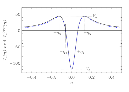
Figure 1: The effective potential $V_{u}(\eta)$ for the perturbation variable $u(\eta)$ as obtained by using the quartic expansion of the scale factor. The values $\eta_{0}=1.01$, $\delta=0$, and $\xi=-2/5$ have been used to derive this plot. The almost undistinguishable dot-dashed curve represents a rational approximation to this potential which is valid in the vicinity of the bounce and that is used in Ref. [12]. Clearly, the potential is well-behaved at all relevant times, and so is the corresponding variable $u$.

Obviously, for such a complicated potential, the equation of motion (4) cannot be solved analytically. However, in the case we are interested in, namely $\Upsilon\ll 1$, the potential has a simple behavior, which can be studied simply by retaining only the smallest order terms in $\Upsilon$.

In the limit where $\Upsilon$ goes to zero, the extremum of the potential $V_{0}$ diverges while its width, characterized by $\eta_{\rm z}$, shrinks to zero, namely

$$V_{0}=-\frac{5\xi}{2\Upsilon}+{\cal O}(\Upsilon^{0}),\quad\eta_{\rm z}=\sqrt{-\frac{\Upsilon}{5\xi}}+{\cal O}(\Upsilon^{3/2}).$$ (8)

This observation is confirmed by a study of the wings in Fig. 1 whose height and position are found to be

$$V_{\rm w}=-\frac{5\xi}{6\Upsilon}+{\cal O}(\Upsilon^{0}),\quad\eta_{\rm w}=\sqrt{-\frac{4\Upsilon}{5\xi}}+{\cal O}(\Upsilon^{3/2}),$$ (9)

and exhibit therefore a similar behavior in the NEC-preserved short time limit. The previous properties suggest that we deal with a distributional effective potential, and indeed, a more careful analysis reveals that [12]

$$V_{u}(\eta)=-C_{\Upsilon}\Delta_{\Upsilon}(\eta),$$ (10)

where the constant $C_{\Upsilon}$ is given by $C_{\Upsilon}\equiv[-5\pi^{2}\xi/(8\Upsilon)]^{1/2}$ and where the function $\Delta_{\Upsilon}(\eta)$ is a representation of the Dirac $\delta$-function, i.e. $\lim_{\Upsilon\rightarrow 0}\Delta_{\Upsilon}(\eta)=\delta(\eta)$. Note that even though the potential appears singular, this is nothing but a computational trick allowing an easy derivation of the resulting spectrum (recall that in realistic situations, the parameter $\Upsilon$ must remain small but nonvanishing [12]). The equation of motion (4) of the quantity $u$ can now be written as

$$u^{\prime\prime}+[n(n+2)+C_{\Upsilon}\delta(\eta)]u=0,$$ (11)

which is nothing but a Schrödinger-like equation for a distributional potential. Right before (superscript $<$) and after (superscript $>$) the point $\eta=0$, but still within the bounce epoch, a Fourier mode does not interact with the barrier since the potential vanishes and the solutions are just linear combinations of plane waves $\mathrm{e}^{i\sqrt{n(n+2)}\eta}$ and $\mathrm{e}^{-i\sqrt{n(n+2)}\eta}$ with coefficients $A^{>}$, $B^{>}$ and $A^{<}$, $B^{<}$ before and after the bounce respectively.

In order to calculate what is the spectrum after the bounce, being given some initial conditions before the bounce, one must apply junction conditions. In the case at hand, the matching conditions are $[u]\equiv u(0^{+})-u(0^{-})=0$ and $[u^{\prime}]=-C_{\Upsilon}u(0)$, the last one coming from an integration of the equation of motion in a thin shell around $\eta=0$. This reduces to

$$A^{>}+B^{>} = A^{<}+B^{<},$$ (12)

$$A^{>}-B^{>} = A^{<}-B^{<}-\frac{C_{\Upsilon}(A^{<}+B^{<})}{i\sqrt{n(n+2)}}.$$ (13)

In the limit $\Upsilon\rightarrow 0$, the constant $C_{\Upsilon}$ diverges and therefore the second term in Eq. (13) is dominant. Straightforward algebraic manipulation allows us to determine the transfer matrix defined by [9]

$$\begin{pmatrix}A^{>}\cr B^{>}\end{pmatrix}=T_{u}\begin{pmatrix}A^{<}\cr B^{<}\end{pmatrix},$$ (14)

and we obtain the following expression

$$T_{u}=-i\sqrt{\frac{-5\pi^{2}\xi}{32n(n+2)}}\begin{pmatrix}1&1\cr-1&-1\end{pmatrix}\frac{1}{\Upsilon^{1/2}}.$$ (15)

Some comments are in order at that point. First, one sees that, as discussed above, the transfer matrix depends on the wavenumber. Our calculation permits to actually predict accurately what the dependence is: $\propto[n(n+2)]^{-1/2}$. Moreover, the calculation also predicts the dependence of the transfer matrix on the parameter $\xi$ (except in the limit $\xi\to 0$ for which a different calculation must be done [12]). A point worth mentioning is that the overall amplitude diverges as $\Upsilon\rightarrow 0$. Since $u$ is just a mathematically convenient variable, this is not necessarily problematic. Indeed, using the relation between $u$ and the Bardeen potential $\Phi$, and the fact that, at the bounce, Eq. (2) holds, one can show that the spectrum of the Bardeen potential is perfectly finite after the bounce, even in the limit $\Upsilon\rightarrow 0$. Note also that the fact that relevant scales may be larger than the duration of the bounce itself does not preclude them to be affected by the transition. Finally, it is worth mentioning that the above result has been recovered in Ref. [12] using a different method, including the numerical factor in the overall amplitude.

In more standard situations, even though the amplitude of $\Phi$ might change, the curvature perturbation on uniform density hypersurfaces, i.e. the quantity called $\zeta_{{}_{\mathrm{BST}}}$ [13], does not. Indeed, it satisfies [14]

$$\frac{\zeta_{{}_{\mathrm{BST}}}^{\prime}}{{\cal H}}\propto\left[\frac{1}{3}\left(\frac{k}{{\cal H}}\right)^{2}\left(\frac{\Phi^{\prime}}{{\cal H}}+\Phi\right)+\frac{\kappa a^{2}}{2{\cal H}^{2}}\delta p_{\mathrm{nad}}\right],$$ (16)

which was been shown [13] to hold independently of the gravitational field equations. Eq. (16) implies that $\zeta_{{}_{\mathrm{BST}}}$ is conserved under the conditions that there is no entropy perturbation ($\delta p_{\mathrm{nad}}=0$), the decaying mode of $\Phi$ is neglected, and the scales are super-Hubble ($k\ll{\cal H}$). Since ${\cal H}=0$ at the bounce, the Hubble radius is larger than any relevant scale during a finite interval around the bounce, i.e. cosmological scales are not large in the super-Hubble sense. Through the bounce, moreover, the notion of decaying and growing modes is irrelevant. Two conditions out of three being violated, $\zeta_{{}_{\mathrm{BST}}}$ has no reason to be conserved, and hence is not convenient for describing a bouncing transition. One should note, additionnally, that since the spectrum of $\Phi$ is altered, there is no reason why $\zeta_{{}_{\mathrm{BST}}}$ should not be also spectrally distorted through a bounce.

In this letter, we have demonstrated that there is no reason to believe that the spectrum of large scale cosmological fluctuations is not affected by a short duration bounce, although this is not necessarily the case (one could choose for instance $\eta_{0}\gg 1$, however hard this is to reconcile with the field theoretical treatment [12] or have a “slow-roll” kind of bounce with $\eta_{0}=1$ [7]). We have shown that this occurs when one approaches the NEC violation and we have also demonstrated that this effect does not violate causality. This result may find important applications: although the calculation discussed here is based on general relativity, there is no reason why causality should act differently in the framework of, say, string theory. In string motivated cosmological scenarios (as for instance in the pre-big bang paradigm [3] or in the ekpyrotic case [5]), the calculation of the power spectrum of cosmological fluctuations is done in the contracting phase and the predictions relevant for observational purposes then stems from the assumption that for sufficiently large scales, perturbations are essentially not affected by the bounce. Our result indicates that this assumption is far from trivial and may challenge the conclusions reached so far in the literature.

We wish to thank R. Brandenberger, A. Buonanno and particularly F. Finelli and D. J. Schwarz for enlightening discussions over many points discussed in this paper.

References

- [1] J. Polchinski, String theory, Cambridge University Press (Cambridge, 1998); M. B. Green, J. H. Schwarz, and E. Witten, Superstring theory, Cambridge University Press (Cambridge, 1987); E. Kiritsis, Introduction to superstring theory, hep-th/9709062.
- [2] T. Banks, M-theory and cosmology, Les Houches summer school, Eds. P. Binétruy et al., Elsevier Science Publishers (2001) and references therein.
- [3] See M. Gasperini and G. Veneziano, Phys. Rep. 373, 1 (2003) and references therein.
- [4] R. Kallosh, L. Kofman, and A. Linde, Phys. Rev. D64, 123523 (2001); R. Kallosh, L. Kofman, A. Linde, and A. Tseytlin, Phys. Rev. D64, 123524 (2001); D. H. Lyth, Phys. Lett. B 524, 1 (2002); R. Brandenberger and F. Finelli, JHEP 0111, 056 (2001); J. Hwang, astro-ph/0109045; D. H. Lyth, Phys. Lett. B 526, 173 (2002); J. Martin, P. Peter, N. Pinto-Neto, and D. J. Schwarz, Phys. Rev. D65, 123513 (2002); ibid 67, 028301 (2003), and references therein.
- [5] J. Khoury, B. A. Ovrut, P. J. Steinhardt, and N. Turok, Phys. Rev. D64, 123522 (2001); J. Khoury, B. A. Ovrut, P. J. Steinhardt, and N. Turok, [hep-th/0105212]; J. Khoury, B. A. Ovrut, N. Seiberg, P. J. Steinhardt, and N. Turok, Phys. Rev. D65, 086007 (2002); J. Khoury, B. A. Ovrut, P. J. Steinhardt, and N. Turok, Phys. Rev. D66, 046005 (2002); R. Durrer, [hep-th/0112026].
- [6] P. Peter and N. Pinto-Neto,Phys. Rev. D66, 063509 (2002); J. C. Fabris, R. G. Furtado, P. Peter, and N. Pinto-Neto, Phys. Rev. D67, 124003 (2003); C. Cartier, R. Durrer, and E. J. Copeland, Phys. Rev. D67, 103517 (2003); P. Peter and N. Pinto-Neto, hep-th/0306005; M. Gasperini, M. Giovannini, and G. Veneziano, hep-th/0306113.
- [7] C. Gordon and N. Turok, Phys. Rev. D67, 123508 (2003).
- [8] R. Brustein and R. Madden, Phys. Rev. D57, 712 (1998); S. Foffa, M. Maggiore, and R. Sturani, Nucl. Phys. B 552, 395 (1999); C. Cartier, E. J. Copeland, and R. Madden, JHEP 01, 035 (2000).
- [9] R. Durrer and F. Vernizzi, Phys. Rev. D66, 083503 (2002).
- [10] V. F. Mukhanov, H. A. Feldman, and R. H. Brandenberger, Phys. Rep. 215, 203 (1992).
- [11] F. Finelli and R. Brandenberger, Phys. Rev. Lett. 82, 1362 (1999); Phys. Rev. D62 083502 (2000).
- [12] J. Martin and P. Peter, Phys. Rev. D103517, (2003).
- [13] D. Wands, K. A. Malik, D. H. Lyth, and A. R. Liddle, Phys. Rev. D62, 043527 (2000).
- [14] J. Martin and D. J. Schwarz, Phys. Rev. D57, 3302 (1998).