Preparing Red-Green-Blue (RGB) Images from CCD Data

Abstract

We present a new, and we believe arguably correct, algorithm for producing Red-Green-Blue (RBG) composites from 3-band astronomical images. Our method ensures that an object with a specified astronomical color (e.g. $g-r$ and $r-i$) has a unique color in the RGB image, as opposed to the burnt-out white stars to which we are accustomed. A natural consequence of this is that we can use the same colors to code color-magnitude diagrams, providing a natural ‘index’ to our images.

We also introduce the use of an asinh stretch, which allows us to show faint objects while simultaneously preserving the structure of brighter objects in the field, such as the spiral arms of large galaxies.

We believe that, in addition to their aesthetic value, our images convey far more information than do the traditional ones, and provide examples from Sloan Digital Sky Survey (SDSS) imaging, the Hubble Deep Field (HDF), and Chandra to support our claims. More examples are available at http://www.astro.princeton.edu/$\sim$rhl/PrettyPictures.

1 Introduction

The purest and most thoughtful minds are those which love colour the most

One of the reasons that our forbears were drawn to astronomy was the sheer drama and beauty of the night sky. When photography became a standard astronomical technique, it was natural to combine images taken in different bands to produce spectacular colored images of the night sky (e.g. Malin, (1992) and references therein).

When CCD detectors were introduced into astronomy 25 years ago, and especially when large-format cameras became common, astronomers were once again motivated to generate 3-color composites. CCDs are approximately linear, unlike the roughly logarithmic sensitivity curve of photographic plates, so the natural way to produce an image was to map the logarithm of the pixel intensities to the red, green, and blue brightnesses in the final image (see e.g. Villard and Levay, (2002)). This algorithm produces pictures that look rather like those produced from photographs, but unfortunately it also discards a lot of information.

2 Generating Colored Images from CCD Data

Let us consider CCD data taken in three bands which we shall call $b$, $g$, and $r$ (E.g. $B$, $R$, and $I$); we assume that these data have been background-subtracted, if necessary linearised, flatfielded, and scaled appropriately. This scaling is to some extent arbitrary, as different astronomers prefer different color balances, but we have found that a conversion to $f_{\nu}$ (in practice to an AB scale, Oke and Gunn, (1983)) works well.

We desire a mapping to the range $[0,1]$ for each of three colors red (R), green (G), and blue (B). The usual algorithm is:

$$R=f(r);\,G=f(g);\,B=f(b)$$ (1)

where

$$f(x)=\cases{0,&$x<m$;\cr F(x-m)/F(M-m)&$m\leq x\leq M$;\cr 1&$M<x$.}$$

and $m$ is the minimum value to display, and $M$ the maximum; these are chosen to bring out favoured details. As mentioned in the introduction, a common choice is logarithmic ($F\equiv\ln$), but linear or square-root stretches are also popular. The actual implementation, at least for integer input data, often uses a lookup table.

This style of mapping simulates one of the unfortunate features of photographic plates, namely that all pixels for which $r$, $g$, and $b$ are $\geq M$ appear white in the final image. In a photograph this white color corresponds to a lack of information, but for a CCD it is a choice made by the astronomer. In fact, for any non-linear function $F$, an object’s color in the composite image depends upon its brightness, even if none of $r$, $g$, or $b$ exceed $M$.

Fortunately, we can easily avoid these problems. Defining $I\equiv(r+g+b)/3$ , set

$$R =r*f(I)/I$$

$$G =g*f(I)/I$$ (2)

$$B =b*f(I)/I$$

If $\max_{RGB}\equiv\max(R,G,B)>1$, set $R\equiv R/\max_{RGB}$, $G\equiv G/\max_{RGB}$, and $B\equiv B/\max_{RGB}$; if $I\equiv 0$, set $R=G=B=0$. In other words, the intensity is clipped at unity, but the color is correct. Additionally, it is possible to choose a more flexible functional form for $F$; following Lupton et al., (1999), we take $F(x)\equiv\textrm{asinh}(x/\beta)$, where the softening parameter $\beta$ is chosen to bring out desired details — it determines the point at which we change from a linear to a logarithmic transformation ($\textrm{asinh}(x)\sim x$ for $x\ll 1$; $\textrm{asinh}(x)\sim\ln(2x)$ for $x\gg 1$) . The linear part is used to show faint features in the data, while the logarithmic part enables us to simultaneously illustrate structures such as spiral arms or the cores of star clusters that are significantly brighter. As an additional trick, we find that sometimes a $\sqrt{\textrm{asinh}}$ stretch brings out the details of dust lanes in spiral galaxies; here, as before, the asinh is used to control the dynamic range.

The results of this simple change are dramatic; a given color (i.e. value of $g-b$ and $r-g$) is now mapped to a unique color in the RGB image. Fig. 1 shows an SDSS (York et al.,, 2000) g-r-i composite of the galaxies NGC6976, NGC6977, and NGC6978. The reader will notice that the stars, rather than all being white, show a variety of red, yellow, and bluish tints; that the spiral bulges (and the group of ellipticals to the lower right of NGC6977) are a uniform yellowish color, while the spiral disks are blue ($[OIII]$ and $H_{\alpha}$ appear in B and R respectively). Furthermore, it is evident that star formation activity in the disks (as indicated by the distinctive bluish color) decreases from left to right.

We may use the well-known color composite of the Hubble Deep Field (HDF; Williams et al, (1996)), Fig. 6, as a pedagogical example. The top row of images were prepared using using Eq. 1, while the bottom row used Eq. 2. The top left panel shows the familiar STScI color image. The bottom left panel use an asinh stretch, and is our preferred representation of the HDF. The top middle panel is our best match to the STScI image and uses a logarithmic stretch; the middle bottom panel uses the same logarithmic function (i.e. identical values of $m$ and $M$). The righthand pair of panels share a hard linear stretch (it is identical to the linear part of the asinh stretch of the bottom left panel).

Interestingly, the bottom set of panels are pretty similar, with the main difference being that the spiral arms in the lower left corner are rather better defined in the leftmost panel. It is clear that much of the morphological information is carried in the color rather than the intensity.

The bands ($f450$, $f606$, and $f814$) used in Fig. 6 are not quite the same as those used in the SDSS composites ($g$, $r$, and $i$) but the astrophysical palette is similar, in the sense that the larger HDF galaxies have colors similar to those seen in Fig. 1, with blue disks and yellowish bulges. The fainter objects, however, look unlike anything seen in SDSS imaging, with bright red (K-corrected) bulges and, in some cases, bluish disks which must be due to active star formation and the emission of far-uv light.

Fig. 3 shows the globular cluster NGC2419; Fig. 4 shows a color-magnitude diagram of point sources in a 0.6 square degree region surrounding the cluster; the points in this diagram have the same color as the corresponding objects in the image; the cluster horizontal- and giant branches stand out.

Finally, this technique is not restricted to optical data; Fig. 7 shows a Chandra X-ray image of the supernova remnant Cas A.

3 Detector Saturation

Although CCDs are wonderful detectors, they are not perfect. The SDSS data processing pipeline (Lupton et al.,, 2001) interpolates over saturation trails, which accounts for their absence from these images. Unfortunately, it is not able to correctly recover the counts in the cores of saturated stars, but we do know which pixels were involved.

Eq. 2 means that every pixel in the image preserves its color, even in the saturated cores of stars. We can avoid undesirable artifacts in the final picture by finding connected pixels which were saturated in at least one band, and replacing them with the average color of the pixels touching the saturated region. Because we do not wish to average over the long bleed-trails produced by bright stars, we only apply this procedure to saturated pixels with intensities $>M$. An obvious example of a bright star is seen at the bottom right of Fig. 3; in this case we treated all pixels with at least 10000 counts in any band as ‘saturated’.

4 Practical Implementations

The original implementation of these algorithms was included in the SDSS image processing code, but fortunately stand-alone versions are also available. An IDL version is available from http://cosmo.nyu.edu/hogg/visualization/rgb/, and a C version from http://www.sdss.jhu.edu/doc/jpeg.html.

5 Conclusions

Color images have traditionally been considered a luxury, but with the techniques espoused in this paper, we have found that they convey an enormous amount of information. For example, star-forming regions have a distinctive color, and it is very clear, looking at images of spiral galaxies, how much the star formation rate varies. We encourage the reader to visit    http://www.astro.princeton.edu/$\sim$rhl/PrettyPictures where, among other objects, all of the NGC galaxies in the SDSS DR1 (Abazajian et al.,, 2003) are presented.

RHL thanks Michael Strauss for helpful comments on an early version of this manuscript.

Funding for the creation and distribution of the SDSS Archive has been provided by the Alfred P. Sloan Foundation, the Participating Institutions, the National Aeronautics and Space Administration, the National Science Foundation, the U.S. Department of Energy, the Japanese Monbukagakusho, and the Max Planck Society. The SDSS Web site is http://www.sdss.org/.

The SDSS is managed by the Astrophysical Research Consortium (ARC) for the Participating Institutions. The Participating Institutions are The University of Chicago, Fermilab, the Institute for Advanced Study, the Japan Participation Group, The Johns Hopkins University, Los Alamos National Laboratory, the Max-Planck-Institute for Astronomy (MPIA), the Max-Planck-Institute for Astrophysics (MPA), New Mexico State University, University of Pittsburgh, Princeton University, the United States Naval Observatory, and the University of Washington.

6 Figures

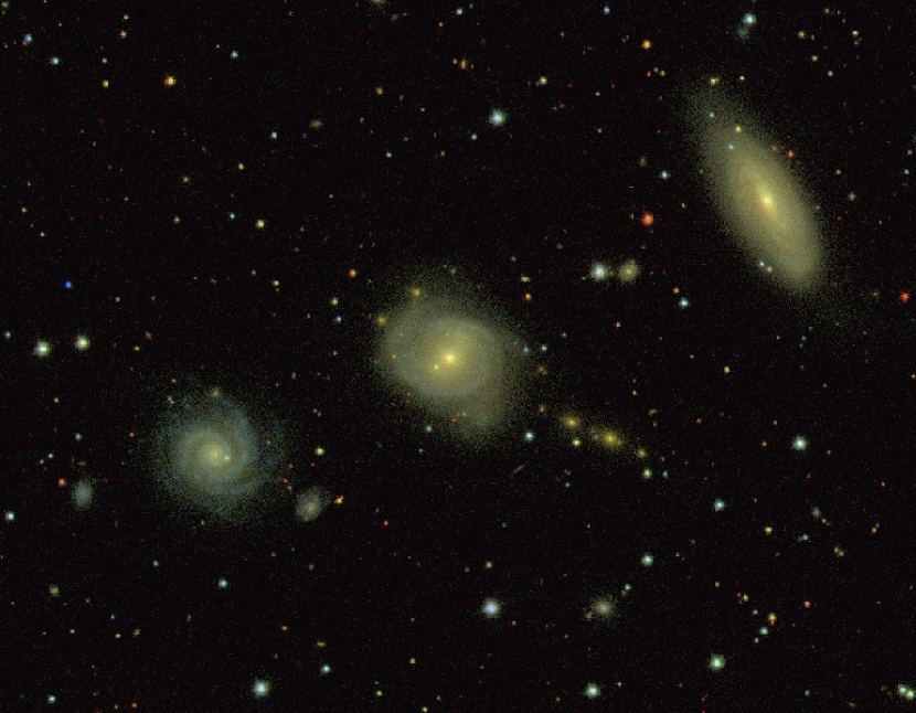
Figure 1: An approximately $5^{\prime}\times 6.5^{\prime}$ g-r-i composite based on SDSS imaging of the galaxies NGC6976, NGC6977, and NGC6978. The faintest objects visible in this image have $r\sim 22$. Note the colors of the stars, ranging from bluish through yellow to red, the blue spiral disks, and the yellowish color of the galaxies spheroids. The stretch is asinh with $Q\equiv 8$ and $\alpha\equiv 0.02$.

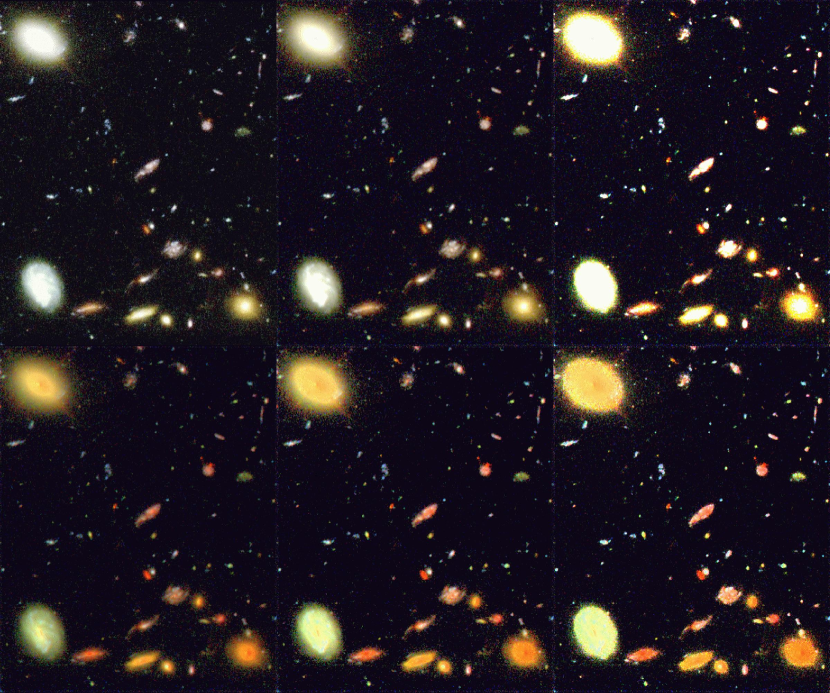
Figure 2: A $f450$, $f606$, and $f814$ composite of the HDF . The top row of images were prepared using using Eq. 1, while the bottom row used Eq. 2. The top left panel shows the familiar STScI color image. The bottom left panel use an asinh stretch, and is our preferred representation of the HDF. The top middle panel is our best match to the STScI image and uses a logarithmic stretch; the middle bottom panel uses the same logarithmic function (i.e. identical values of $m$ and $M$). The righthand pair of panels share a hard linear stretch (it is identical to the linear part of the asinh stretch of the bottom left panel). In the bottom row of images, the larger galaxies have similar colors to the galaxies in Fig. 1, but the fainter, more distant, red galaxies have no analogues in the shallow SDSS data; our eyes are seeing the effects of redshifting the 4000Å break.

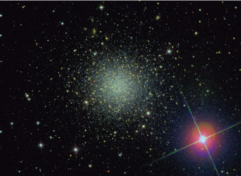
Figure 3: An approximately $7^{\prime}\times 9^{\prime}$ g-r-i composite based on SDSS imaging of the halo globular cluster NGC2419. Note the blue horizontal branch and yellowish red giants; the red stars are M-stars in the disk. The diffraction spikes show that the instrument rotator moved significantly during the 5 minutes between the $g$ and $r$ exposures. The stretch is asinh with $Q\equiv 9$ and $\alpha\equiv 0.02$.

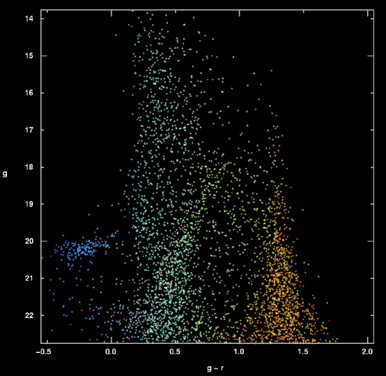
Figure 4: A $g-r$ v. g color-magnitude diagram for stars in an area of about 0.6 square degrees around the cluster NGC2419. Each star has the same color as it has is in a gri composite image of that part of the sky, a part of which is shown in Fig. 3.

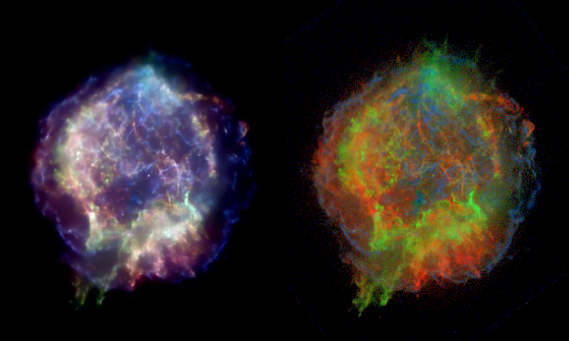
Figure 5: The Supernova remnant Cas A, as imaged by the Chandra X-ray satellite using the ASIS camera . R, G, and B correspond to 0.3—1.55 keV, 1.55—3.34 keV, and 3.34—10keV respectively. The lefthand image is from the Chandra Supernova Catalog, the righthand image is prepared using Eq. 2 and an asinh stretch. The input image is the raw Chandra data smoothed with a sigma=0.5pixel Gaussian; this is not the same as the inputs to the left hand panel. Note the presence of both blue and red filaments crossing the center of the remnant. It is possible to generate a figure analogous to Fig. 4 that shows the mapping from hardness ratios to RGB.

References

- Abazajian et al., (2003) Abazajian, K., et al., 2003, AJ 126, 2081.
- Lupton et al., (1999) Lupton, R. H., Gunn, J. E. & Szalay, A. 1999, AJ 118, 1406.
- Lupton et al., (2001) Lupton, R. H. et al. 2001 ADASS X, 269.
- Oke and Gunn, (1983) Oke, J.B. and Gunn, J.E., 1983. ApJ 266, 713.
- Malin, (1992) Malin, D., 1992. Royal Astron. Soc. Quart. Jrn. 33, 321.
- Villard and Levay, (2002) Villard, R, and Levay, Z 2002. Sky & Telescope 104, V3, 28.
- Williams et al, (1996) Williams, R. E., et al. 1996. AJ 112, 1335.
- York et al., (2000) York et al., 2000 AJ 120 1579.