Alfvénic reacceleration of relativistic particles in galaxy clusters: MHD waves, leptons and hadrons

Abstract

There is a growing evidence that extended radio halos are most likely generated by electrons reaccelerated via some kind of turbulence generated in the cluster volume during major mergers. It is well known that Alfvén waves channel most of their energy flux in the acceleration of relativistic particles. Much work has been done recently to study this phenomenon and its consequences for the explanation of the observed non-thermal phenomena in clusters of galaxies. We investigate here the problem of particle-wave interactions in the most general situation in which relativistic electrons, thermal protons and relativistic protons exist within the cluster volume. The interaction of all these components with the waves, as well as the turbulent cascading and damping processes of Alfvén waves, are treated in a fully time-dependent way. This allows us to calculate the spectra of electrons, protons and waves at any fixed time. The Lighthill mechanism is invoked to couple the fluid turbulence, supposedly injected during cluster mergers, to MHD turbulence. We find that present observations of non-thermal radiation from clusters of galaxies are well described within this approach, provided the fraction of relativistic hadrons in the intracluster medium (ICM) is smaller than $5-10\%$.

1 Introduction

There is now firm evidence that the ICM is a mixture of hot gas, magnetic fields and relativistic particles. While the hot gas results in thermal bremsstrahlung X-ray emission, relativistic electrons generate non-thermal radio and hard X-ray radiation. The amount of the energy budget of the intracluster medium in the form of high energy hadrons can be large, due to the phenomenon of confinement of cosmic rays over cosmological time scales (Völk et al. 1996; Berezinsky, Blasi & Ptuskin 1997). Nevertheless, the gamma radiation that would allow us to infer the fraction of relativistic hadrons in clusters has not been detected as yet (Reimer et al., 2003).

The most important evidence for relativistic electrons in clusters of galaxies comes from the diffuse synchrotron radio emission observed in about $35\%$ of the clusters selected with X–ray luminosity $>10^{45}$ erg s^-1 (e.g., Feretti, 2003). The diffuse emission comes in two flavors, referred to as radio halos (and/or radio mini–halos) when the emission appears concentrated at the center of the cluster, and radio relics when the emission comes from the peripherical regions of the cluster.

The difficulty in explaining the extended radio halos arises from the combination of their $\sim$Mpc size, and the relatively short radiative lifetime of the radio emitting electrons. Indeed, the diffusion time necessary for the radio electrons to cover such distances is orders of magnitude larger than their radiative lifetime. As proposed first by Jaffe (1977), a solution to this puzzle would be provided by continuous in situ reacceleration of the relativistic electrons on their way out. This possibility was studied more quantitatively by Schlickeiser et al. (1987) who successfully reproduced the integrated radio spectrum of the radio halo in the Coma cluster. In the framework of the in situ reacceleration model, Harris et al. (1980) first suggested that cluster mergers might provide the energetics necessary to reaccelerate the relativistic particles.

An alternative to the reacceleration scenario was put forward by Dennison (1980), who suggested that relativistic electrons may be produced in situ by inelastic proton-proton collisions through production and decay of charged pions. This model is known in the literature as the secondary electron model.

Diffuse radio emission is not the only evidence of non-thermal activity in the ICM. Additional evidence, although limited to a few cases, comes from the detection of extreme ultra-violet (EUV) excess emission (e.g., Bowyer et al. 1996; Lieu et al., 1996; Berghöfer et al., 2000; Bonamente et al., 2001), and of hard X-ray (HXR) excess emission in the case of the Coma cluster, A2256 and possibly A754 (Fusco–Femiano et al., 1999, 2000, 2003, 2004; Rephaeli et al., 1999; Rephaeli & Gruber, 2002, 2003). While, with the exception of the Coma and Virgo clusters, the detection of EUV emission is still controversial (e.g., Berghöfer et al., 2000), the detection of HXRs appears robust as it is claimed independently by different groups and with different X–ray observatories (BeppoSAX, RXTE). If these excesses are indeed of non-thermal origin, they may be explained in terms of IC scattering of relativistic electrons off the photons of the cosmic microwave background (CMB) (Fusco–Femiano et al., 1999, 2000; Rephaeli et al., 1999; Völk & Atoyan 1999; Blasi 2001; Brunetti et al.2001a; Fujita & Sarazin 2001; Petrosian 2001; Kuo et al., 2003). Alternatively HXRs might also result from bremsstrahlung emission of electrons in the thermal gas whose spectrum is not a perfect Maxwellian, but rather has a supra-thermal tail (e.g., Ensslin, Lieu, Biermann 1999; Blasi 2000; Dogiel 2000; Sarazin & Kempner 2000). Blasi (2000) calculated the spectrum of the electrons as modified by the resonant interaction with MHD waves by solving a time-dependent Fokker-Planck equation and reached the conclusion that the intracluster medium is heated and at the same time develops a supra-thermal tail due to the resonant particle-wave interaction. An energy injection comparable with the whole luminosity of a merger, lasting for about a billion years was required in this calculation (Blasi 2000) in order to explain observations. A shorter allowed duration (about $10^{8}$ years) of the event was estimated by Petrosian (2001).

Both the IC model and the bremsstrahlung interpretation have problems: the first one would require cluster magnetic field strengths smaller than those inferred from measurements of the Faraday rotations (e.g., Carilli & Taylor 2002). The second one would require a large amount of energy to maintain a substantial fraction of the thermal electrons far from the thermal equilibrium for more than a few $10^{8}$yrs (Blasi, 2000; Petrosian, 2001).

The origin of radio halos is still an open problem. In principle, it is known that the fine radio properties of the radio halos may be naturally accounted for in models in which electrons are directly accelerated (primary electrons) whereas they are difficult to reproduce in models in which the electrons are secondary products of hadronic interactions (Brunetti, 2002). On the other hand, the details of the physics used in the primary electron models are relatively uncertain. In principle, merger shocks can accelerate relativistic electrons to produce large scale synchrotron radio emission (e.g., Roettiger et al., 1999; Sarazin 1999; Takizawa & Naito, 2000), however, the radiative life–time of the emitting electrons diffusing away from these shocks is so short that they would just be able to produce relics and not Mpc scale radio halos (e.g., Miniati et al, 2001). In addition, a number of papers (Gabici & Blasi 2003; Berrington & Dermer 2003) have recently pointed out that the Mach number of the typical shocks produced during major merger events is too low to generate non–thermal radiation with the observed fluxes and spectra.

Re–acceleration of a population of relic electrons by turbulence powered by major mergers is suitable to explain the very large scale of the observed radio emission and is also a promising possibility to account for the fine radio structure of the diffuse emission (Brunetti et al., 2001a,b). There are a number of possibilities to channel the energy of the turbulence in the acceleration of fast particles, namely via Magneto-Sonic (MS) waves, via magnetic Landau damping (e.g., Kulsrud & Ferrari 1971), via Lower Hybrid (LH) waves (e.g., Eilek & Weatherall 1999) or via Alfvén waves. Since Alfvén waves are likely to be able to transfer most of their energy into relativistic particles, they have received much attention in the last few years. In this framework for instance Ohno, Takizawa and Shibata (2002) developed a time-independent model for the acceleration of the relativistic electrons expected in radio halos through magnetic turbulence. The authors studied the acceleration of continuously injected relativistic electrons by Alfvén waves with a power law spectrum and applied this model to the case of the radio halo in the Coma cluster. More recently, Fujita, Takizawa and Sarazin (2003) studied the effect of Alfvénic acceleration of relativistic electrons in clusters of galaxies. These authors invoked the Lighthill theory to establish a connection between the large scale fluid turbulence and the radiated MHD waves. The electron and MHD-wave spectra adopted by Fujita et al.(2003) are obtained via a self-similar approach by requiring that the spectra are described by two power laws.

These approaches have two intrinsic limitations: the first one is in the assumption, mentioned above, that all spectra are time-independent and that the turbulence spectrum is a power law. The second is that they neglect, as all other previous approaches did, the effect of relativistic hadrons in the ICM: it is well known that the interaction of the Alfvén waves with relativistic particles is, in general, more effective for protons than for electrons (e.g., Eilek 1979). It is also well known that the presence of a significant energy budget in the form of relativistic particles can significantly affect the spectrum of the Alfvén waves through damping. In fact, this damping occurs even on the thermal protons in the ICM, another effect which was never included in previous calculations.

The calculations presented here provide a self-consistent time-dependent treatment of the non-linear coupling of Alfvén waves, relativistic electrons, thermal and relativistic protons. The results previously appeared in the literature can be obtained as special cases of our very general approach, which is in principle applicable to scenarios other than clusters of galaxies.

The paper is organized as follows: in Sect. 2 we discuss the energy losses of relativistic particles and the presence of these particles in galaxy clusters. In Sect. 3 we discuss the physics of Alfvén waves, their generation in galaxy clusters and their interaction with particles. In Sect. 4 we discuss the physics of the coupling between Alfvén waves, leptons and hadrons and derive the time evolution of waves and particles as a function of the physical conditions typical of the ICM. In Sect. 5 we apply our general formalism to calculate the fluxes of radio radiation and hard X–ray tails in galaxy clusters.

Throughout the paper we adopt $H_{0}=50$ km s^-1 Mpc^-1; if not specified all the quantities are given in c.g.s. units.

2 Basic equations and assumptions

2.1 Energy losses of relativistic particles in the ICM

In this Section we give a short summary of the main energy loss channels that may be important for electrons and protons in the ICM.

2.1.1 Electrons

Relativistic electrons with momentum $p=m_{\rm e}c\gamma$ in the ICM lose energy through ionization losses and Coulomb collisions (Sarazin 1999):

$$\left({{dp}\over{dt}}\right)_{\rm i}=-3.3\times 10^{-29}n_{\rm th}\left[1+{{{\rm ln}(\gamma/{n_{\rm th}})}\over{75}}\right]$$ (1)

where $n_{\rm th}$ is the number density of the thermal plasma. Relativistic electrons lose energy via synchrotron emission and inverse Compton scattering (ICS):

$$\left({{dp}\over{dt}}\right)_{\rm rad}=-4.8\times 10^{-4}p^{2}\left[\left({{B_{\mu G}}\over{3.2}}\right)^{2}{{\sin^{2}\theta}\over{2/3}}+(1+z)^{4}\right]$$ (2)

where $B_{\mu G}$ is the magnetic field strength in $\mu G$ and $\theta$ is the pitch angle of the emitting electrons; in case of efficient isotropization of the electron momenta it is possible to average over all possible pitch angles, so that $<\sin^{2}\theta>=2/3$. It is well known that in the typical conditions of the ICM radiation losses are the most important for electrons with Lorentz factor $\gamma\gg 100$ while Coulomb losses dominate at lower energies (Sarazin 1999,2001; Brunetti 2002). The lifetime of relativistic electrons, defined as $\tau\sim\gamma/\dot{\gamma}$, can be easily estimated from Eqs.(1–2) as:

$$\tau_{\rm e}({\rm Gyr})\sim 4\times\Big{\{}{1\over 3}\Big{(}{{\gamma}\over{300}}\Big{)}\left[\left({{B_{\mu G}}\over{3.2}}\right)^{2}{{\sin^{2}\theta}\over{2/3}}+(1+z)^{4}\right]$$

$$+\Big{(}{{n_{\rm th}}\over{10^{-3}}}\Big{)}\Big{(}{{\gamma}\over{300}}\Big{)}^{-1}\left[1.2+{1\over{75}}\ln\Big{(}{{\gamma/300}\over{n_{\rm th}/10^{-3}}}\Big{)}\right]\Big{\}}^{-1}.$$ (3)

2.1.2 Protons

The main channel of energy losses for relativistic protons is represented by inelastic proton-proton collisions. The timescale associated with this process is :

$$\tau_{pp}={1\over{{n_{\rm th}\sigma_{\rm pp}c}}}\sim 10^{18}\Big{(}{{n_{\rm th}}\over{10^{-3}}}\Big{)}^{-1}~{}.$$ (4)

Inelastic ${\rm pp}$ scattering is weak enough to allow for the accumulation of protons over cosmological times (Berezinsky, Blasi & Ptuskin 1997). The rare interactions with the ICM may generate an appreciable flux of gamma rays and neutrinos, in addition to a population of secondary electrons (Blasi & Colafrancesco 1999). The process of pion production in $pp$ scattering is a threshold reaction that requires protons with kinetic energy larger than $\sim 300$ MeV.

Protons which are more energetic than the thermal electrons, namely protons with velocity $\beta>\beta_{c}=(3/2m_{e}/m_{p})^{1/2}\beta_{e}$ ($\beta_{e}$ here is the velocity of the thermal electrons, $\beta_{e}\simeq 0.18(T/10^{8}K)^{1/2}$) lose energy due to Coulomb interactions. If we define $x_{m}=\left({{3\sqrt{\pi}}\over{4}}\right)^{1/3}\beta_{e}$, we can write (e.g., Schlickeiser, 2002):

$${{dp}\over{dt}}\simeq-1.7\times 10^{-29}\left({{n_{\rm th}}\over{10^{-3}}}\right){{\beta}\over{x_{m}^{3}+\beta^{3}}}$$ (5)

with the following asymptotic behaviour:

$${{dp}\over{dt}}\propto\left({{n_{\rm th}}\over{10^{-3}}}\right)\times\left\{\begin{array}[]{lll}\textrm{Const.}&\textrm{for}&p>>mc\\ p^{-2}&\textrm{for}&mcx_{m}<p<<mc\\ p&\textrm{for}&mc\beta_{c}<p<mcx_{m}\end{array}\right.$$ (6)

The timescale associated with Coulomb collisions (in the case $mcx_{m}<p\ll mc$) can be therefore written as:

$$\tau_{C}\sim 2.5\times\tau_{pp}\Big{(}{{p}\over{m_{\rm p}c}}\Big{)}^{3}.$$ (7)

For trans-relativistic and sub-relativistic protons this channel can easily become the main channel of energy losses in the ICM.

2.2 Origin and spectrum of the relic relativistic particles

In this section we briefly discuss the mechanisms responsible for the injection of cosmic rays in galaxy clusters, more extended discussions have been previously presented by Berezinsky, Blasi & Ptuskin (1997), Kronberg (2002), Biermann et al. (2002) and Jones et al. (2002).

Collisionless shocks are generally recognized as efficient particle accelerators through the so-called “diffusive shock acceleration” (DSA) process (Drury, 1983; Blandford & Eichler 1987). This mechanism has been invoked several times as the main acceleration process in clusters of galaxies that have been involved in a merger event (Takizawa & Naito, 2000; Blasi 2001; Miniati et al., 2001; Fujita & Sarazin 2001). For the case of standard newtonian shocks, relevant for clusters of galaxies, the spectrum of the accelerated particles can be shown to be a power-law with a slope that is independent of the details of the diffusion in the shock vicinity, and depends only on the compression factor $r$ at the shock, $s=(r+2)/(r-1)$.

The injection of CR ions at shocks is generally computed in the test particle limit while the injection efficiency is sometimes just assumed as a free parameter, while in other cases it is estimated according to the so-called thermal leakage model (e.g., Kang & Jones, 1995).

There is still some debate on the typical Mach number of the shocks developed in the ICM during cluster mergers. Some results from numerical simulations suggest the presence of a large fraction of high Mach number shocks in cluster mergers (Miniati et al., 2000, 2001). Semi–analytical calculations (Gabici & Blasi 2003; Berrington & Dermer 2003) have pointed out that the Mach numbers of the shocks related to major mergers are expected to be of order unity. Recent numerical simulations (Ryu et al., 2003) seem to find more weak shocks than in Miniati et al.(2000, 2001). The comparison however with analytical calculations appears difficult because of a different classification of the shocks in the two approaches. Moreover the numerical simulations of Ryu et al. (2003) also find a class of high Mach number shocks that are related to gravitationally unbound structures, not included in semi-analytical calculations. On the other hand, the weakness of the merger-related shocks seems to be also suggested by the few observations in which the Mach number of the shock can be measured (e.g., Markevitch et al., 2003). If shocks related to major mergers are indeed weak, the spectra of the accelerated particles are typically too steep to be relevant for nonthermal phenomena in clusters of galaxies.

A relevant contribution to the injection of cosmic rays in clusters of galaxies may come from Active Galactic Nuclei (AGN). AGNs indeed inject in the ICM a considerable amount of energy in relativistic particles and also in magnetic fields, likely extracted from the accretion power of their central black hole (Ensslin et al., 1997). It should be stressed that the presence of relativistic plasma in AGNs (radio lobes and jets) is directly observed because of the synchrotron and inverse Compton emission of accelerated electrons.

Finally, powerful Galactic Winds (GW) can inject relativistic particles and magnetic fields in the ICM (Völk & Atoyan 1999). Although the present day level of starburst activity is low, it is expected that these winds were more powerful during starburst activity in early galaxies. Some evidence that powerful GW were more frequent in the past comes from the observed iron abundance in galaxy clusters (Völk et al. 1996).

Figure 1: Electron spectrum at $z=0$ injected as a single burst at $z_{i}=$0.01, 0.1, 0.3, 0.5 (from right to left) adopting injection spectrum $Q(p)\propto p^{-2.5}$ and maximum Lorentz factor $\gamma_{max}=10^{4}$. The calculations are carried out for $n_{th}=10^{-3}$cm^-3 and $B=1\mu$G.

Since most of the scenarios discussed above imply power law spectra of relativistic particles at the injection sites, in the following we will restrict our calculation to this case. It is worth recalling that transport effects and energy losses modify the shape of these spectra, that are not expected to be power laws at later times.

2.2.1 Electron Spectrum

In the conditions typical of the ICM, ultra-relativistic electrons rapidly cool down through ICS and synchrotron emission, and accumulate in the region of Lorentz factors $\gamma\sim 100-500$ where they may stay for a few billion years before cooling further down in energy through Coulomb scattering and eventually thermalize.

The kinetic equation that describes these losses and the continuous injection of electrons is (Kardashev, 1962):

$${{\partial N_{\rm e}(p,t)}\over{\partial t}}={{\partial}\over{\partial p}}\Big{(}({{{dp}\over{dt}}}_{rad}+{{{dp}\over{dt}}}_{i})N_{\rm e}(p,t)\Big{)}+Q_{\rm e}(p)$$ (8)

where ${dp/dt}_{\rm i}$, and ${dp/dt}_{\rm rad}$ are given by Eqs.(1) and (2) respectively and $Q_{\rm e}(p)$ represents the injection term. The time evolution of relativistic electrons in the ICM during cosmological times has been investigated in some detail by Sarazin (1999) by making use of the numerical solutions of Eq. (8). In Fig. 1 we plot the spectrum of relativistic electrons measured at the present time and injected in a single event at $z=z_{i}$ in the cluster volume. The calculations are shown for different values of $z_{i}$: the spectra flatten with increasing $z_{i}$ (typical conditions of the ICM are adopted, as described in the figure caption). Most electrons injected at $z_{i}>0.2$ get thermalized.

In the case of continuous time-independent injection, it is well known that an equilibrium spectrum of the electrons is achieved, that can be written as follows:

$$N_{\rm e}(p,z)\propto\cases{p^{-s({\cal M})+1},&if $p<<p_{\rm eq}(z)$;\cr p^{-s({\cal M})-1}&if $p>>p_{\rm eq}(z)$.\cr}$$ (9)

where $p_{\rm eq}$ is close to the momentum at which the Coulomb losses dominate over the radiative losses, namely:

$$p_{\rm eq}(z)\sim 300\times m_{\rm e}c\Big{(}{{n_{\rm th}}\over{10^{-3}}}\Big{)}^{1/2}(1+z)^{-2}$$ (10)

More realistic injection histories of relativistic electrons can be easily implemented in this kind of calculation.

2.2.2 Protons

Both timescales of energy losses and diffusion out of the cluster volume are larger than the Hubble time for most of the cosmic ray protons in the ICM (Völk et al. 1996; Berezinsky, Blasi & Ptuskin 1997), although the energy at which confinement becomes inefficient is rather sensitive on the adopted diffusion model.

As stressed above, mildly and sub- relativistic protons may be significantly affected by Coulomb energy losses, which in turn change the particle spectrum with respect to the injection spectrum.

Figure 2: Present-epoch spectrum of the cosmic ray protons continuously injected (with $p>0.1\,m_{p}c$) in the ICM starting from $z_{i}$. The spectra are plotted for $s=$2.4 (dotted lines) and 3.0 (solid lines) and for $z_{i}=$0.1, 0.5, 1 (from bottom to top). Calculations are carried out assuming $n_{th}=10^{-3}$cm^-3.

Figure 3: The ratio between the energy density of cosmic ray protons with momentum $p>0.1\,m_{p}c$ at the present time ($z=0$) and the energy density in cosmic rays injected from the redshift $z_{i}=z$ (x-axis) to the present. Calculations are carried out for $s=3.3$ (solid line) and $s=4.0$ (dashed line) and for $n_{th}=10^{-3}$cm^-3.

Figure 4: Energy density in the form of cosmic ray protons in the ICM (arbitrary units) if protons are injected at a constant rate (number of particles per unit time) at $p>0.1\,m_{p}c$ with a power law injection spectrum with slope $s$ (on the x-axis). The time at which injection starts is taken as $z_{i}=1$. The density of the thermal gas is assumed to be $n_{th}=10^{-3}$cm^-3.

Below the threshold for pion production in the $pp$ collisions (or simply by neglecting the effect due to $pp$ collisions), the time evolution of the proton spectrum is described by the following equation:

$${{\partial N_{\rm p}(p,t)}\over{\partial t}}={{\partial}\over{\partial p}}\Big{(}{{{dp}\over{dt}}}_{i}N_{\rm p}(p,t)\Big{)}+Q_{\rm p}(p),$$ (11)

where ${dp/dt}_{i}$ is given by Eq. (5). Adopting the non-relativistic asymptotic behaviour of Eq. 6, the asymptotic solution (for time independent injection) is as follows:

$$N_{\rm p}(p,T)={{K_{\rm p}}\over{n_{\rm th}}}{{p^{-s}}\over{{\cal C}}}\left\{\begin{array}[]{llll}\beta>x_{\rm m}\\ {{p^{3}/m_{\rm p}^{2}c^{2}}\over{s-1}}\Big{\{}1-\Big{(}1+{{3{\cal C}n_{\rm th}T}\over{p^{3}/m_{\rm p}^{2}c^{2}}}\Big{)}^{-{{s-1}\over{3}}}\Big{\}}\\ \\ \beta<x_{\rm m}\\ {{x_{\rm m}^{3}m_{\rm p}c}\over{s-1}}\Big{\{}1-\exp({{n_{\rm th}(1-s)T{\cal C}}\over{x_{\rm m}^{3}m_{\rm p}c}})\Big{\}}\end{array}\right.$$ (12)

where ${\cal C}$ is the constant in Eq. (5) and $T$ is the time elapsed from the beginning of the injection. Eq. (12) presents the following behaviours :

$$N_{\rm p}(p,T)\propto\cases{p^{3-s}&if $p<<p_{*}(T)$ \& $p>m_{\rm p}cx_{\rm m}$\cr p^{-s},&if $p<<p_{*}(T)$ \& $p<m_{\rm p}cx_{\rm m}$\cr p^{-s},&if $p>>p_{*}(T)$;\cr}$$ (13)

where $p_{*}(T)$ is given by :

$$p_{*}(T)\sim 0.7\times\Big{(}{{T}\over{10{\rm Gyr}}}{{n_{\rm th}}\over{10^{-3}}}\Big{)}^{1/3}m_{p}c$$ (14)

In Fig. 2 we plot the spectrum of the protons measured at the present time as obtained solving Eq. (11) numerically under the assumption of a continuous time-independent injection of protons (starting from different $z_{i}$, see caption) in the cluster volume. The proton spectra, largely modified in the trans–relativistic regime by Coulomb losses, has the asymptotic behaviour described by Eq. (13).

Since the energy flux of Alfvén waves, as we show below, is efficiently damped on protons, it is important to estimate the amount of energy stored in the form of protons in the ICM.

In Fig. 3 we plot the ratio between the energy injected in cosmic ray protons (assuming time independent injection starting at redshift $z_{i}$) and the energy stored in the form of supra-thermal protons (here $p>0.1\times m_{p}c$) at the present time for different values of the injected spectral index $s$ (see caption). As expected, the ratio between the energy stored in protons at the present time and the injected energy is smaller for steeper injection spectra, due to the effect of Coulomb losses.

Finally, by assuming that a fixed fraction of the thermal protons in the cluster volume is accelerated to higher energies at a constant rate (starting from $z_{i}=1.0$), in Fig. 4 we plot the energy stored in the cluster at the present time as a function of the slope of the injected spectra $s$.

3 Alfvénic acceleration of relativistic particles

Alfvén waves efficiently accelerate relativistic particles via resonant interaction. The condition for resonance between a wave of frequency $\omega$ and wavenumber projected along the magnetic field $k_{\|}$, and a particle of type $\alpha$ with energy $E_{\alpha}$ and projected velocity $v_{\|}=v\mu$ is (Melrose 1968; Eilek 1979):

$$\omega-\nu{{\Omega_{\alpha}}\over{\gamma}}-k_{\|}v_{\|}=0$$ (15)

where, in the quasi parallel case ($k_{\perp}<<m_{\alpha}\Omega_{\alpha}/p$), $\nu=-1$ and $\nu=1$ for electrons and protons respectively.

The dispersion relation for Alfvén waves in an isotropic plasma with both thermal and relativistic particles can be written as (Barnes & Scargle, 1973):

$$\omega^{2}={{k_{\|}^{2}v_{\rm A}^{2}(1+\eta_{1})}\over{1+{4\over 3}\eta_{2}+v_{\rm A}^{2}c^{-2}(1+\eta_{1})}}$$ (16)

where

$$\eta_{1}={{n_{\rm p,rel}}\over{n_{\rm th}}}+{{m_{\rm e}}\over{m_{\rm p}}}\Big{(}1+{{n_{\rm p,rel}}\over{n_{\rm th}}}\Big{)}$$ (17)

and

$$\eta_{2}={{n_{\rm e,rel}m_{\rm e}<\gamma_{\rm e}>+n_{\rm p,rel}m_{\rm p}<\gamma_{\rm p}>}\over{n_{\rm th}m_{\rm p}}}$$ (18)

Since the number density (and possibly the energy density as well) of the thermal component in the ICM is considerably larger than the corresponding non-thermal component, one can show that $\eta_{1}<<1$ and $\eta_{2}<<1$ so that the dispersion relation [Eq. (16)] becomes $\omega\simeq|k_{\|}|v_{\rm A}$. Combining the dispersion relation of the waves with the resonant condition, Eq. (15), one can derive the resonant wavenumber, $k_{res}$, for a given momentum ($p=mv\gamma$) and pitch angle cosine ($\mu$) of the particles:

$$k_{res}\sim|k_{\|}|={{\Omega m}\over{p}}{1\over{\Big{(}\mu\pm{{v_{\rm A}}\over{v}}\Big{)}}},$$ (19)

where the upper and lower signs refer to protons and electrons respectively. In an isotropic distribution of waves and particles, the particle diffusion coefficient in momentum space is given by (Eilek & Henriksen, 1984):

$$D_{\rm pp}(p,t)={{2\pi^{2}e^{2}v_{\rm A}^{2}}\over{c^{3}}}\int_{k_{min}}^{k_{max}}{{W_{k}(t)}\over{k}}\Big{[}1-\Big{(}{{v_{\rm A}}\over{c}}\mp{{\Omega m}\over{pk}}\Big{)}^{2}\Big{]}dk,$$ (20)

where the minimum wavenumber (maximum scale length) of the waves interacting with particles is given by :

$$k_{min}={{\Omega m}\over{p}}{1\over{\Big{(}1\pm{{v_{\rm A}}\over{v}}\Big{)}}}$$ (21)

and $k_{max}$ is given by the largest wavenumber of the Alfvén waves, limited by the fact that the frequency of the waves cannot exceed the proton cyclotron frequency, namely $\omega<\Omega_{p}$. It follows that $k_{max}\sim\Omega_{p}/v_{A}$ or $k_{max}\sim\Omega_{p}/v_{M}$, $v_{M}$ being the magnetosonic velocity (here we assume $k_{max}\sim\Omega_{p}/v_{M}$).

In the simple case of a power law spectrum of the MHD waves, $W(k)\propto k^{-w}$ (for $k_{o}<k<k_{\rm max}$), Eq. (20) would give:

$$D_{\rm pp}(p)=A_{w}(\delta B)^{2}v_{A}^{2}\left({{p}\over{B}}\right)^{w}\Big{(}1\pm{{v_{A}}\over{c}}\Big{)}^{w}\times$$

$$\left\{{1\over{w}}\pm{{v_{A}/c}\over{w+1}}-{{(v_{A}/c)^{2}}\over{w(w+1)}}\right\},$$ (22)

where

$$\delta B^{2}=8\pi\int W_{k}dk,$$ (23)

and

$$A_{w}={{\pi}\over{2}}{{e^{2-w}}\over{c^{3-w}}}{{w-1}\over{w+2}}k_{o}^{w-1}$$ (24)

The first order expansion (for $v_{A}/c<<1$) of Eq. 22 is the diffusion coefficient generally used in most recent theoretical papers on electron acceleration in galaxy clusters (Ohno et al. 2002; Fujita et al. 2003).

3.0.1 Electrons

From Eq. (19), one can see that the momentum of the electrons which can resonate with waves with a given wavenumber $k$ depends on the pitch angle cosine $\mu$. This resonant momentum can be written as

$$p={{\Omega_{e}m_{e}}\over{k}}{1\over{\mu-{{v_{A}}\over{v}}}}.$$ (25)

The minimum momentum of the electrons for which resonance with waves of a given wavenumber $k$ can occur is:

$$p_{min}={{m_{e}}\over{k}}\Big{(}\Omega_{e}+v_{A}k\Big{)},$$ (26)

which, in the relativistic limit becomes:

$$p_{min}^{rel}={{\Omega_{e}m_{e}}\over{k}}{1\over{1-{{v_{A}}\over{c}}}}.$$ (27)

Since the wavenumber of Alfvén waves in a plasma is limited by $\omega<\Omega_{p}$, from Eq. (26), one has that the minimum momentum of the electrons which can resonate with Alfvén waves is:

$$p_{min}=p_{th}{{v_{A}}\over{v_{th}}}\Big{(}{{m_{p}}\over{m_{e}}}+1\Big{)},$$ (28)

which, in general, gives $p_{min}>>p_{th}$, $p_{th}=m_{e}v_{th}$ being the momentum of the thermal electrons. It follows the well known result that thermal electrons cannot resonate with Alfvén waves (Hamilton & Petrosian, 1992 and references therein).

This important limitation of Alfvén waves as particle accelerators forces us to consider the situation in which a relic population of relativistic electrons exists in the ICM (Sect. 2.2), and no electron acceleration from the thermal background is taken into account.

In the case of an isotropic, homogeneus phase–space density electron plasma, the evolution of the electron spectrum can be described in the context of the Fokker–Planck equation (Tsytovich 1966; Borovsky & Eilek 1986):

$${{\partial f(p,t)}\over{\partial t}}={1\over{p^{2}}}{{\partial}\over{\partial p}}\Big{[}D_{\rm pp}p^{2}{{\partial f(p,t)}\over{\partial p}}+{{dp}\over{dt}}_{\rm rad}p^{2}f(p)+$$

$$+{{dp}\over{dt}}_{\rm i}p^{2}f(p)\Big{]}+q^{+}_{e}(p,t),$$ (29)

where $f(p,t)$ is the phase space density of electrons, $D_{\rm pp}$ is the diffusion coefficient due to the interaction with the waves [Eq. (20)], ${dp/dt}_{\rm i}$ and ${dp/dt}_{\rm rad}$ give the ionization and radiative losses [Eq. (1-2)], and $q^{+}_{e}(p,t)$ is an isotropic phase–space electron source term. For simplicity we can introduce the two functions $N(p,t)$ and $Q_{e}(p,t)$, related to $f$ and $q^{+}_{e}$ through the following relations:

$$N(p,t)=4\pi p^{2}f(p,t),$$ (30)

and

$$Q_{e}(p,t)=4\pi p^{2}[q^{+}_{e}(p,t)].$$ (31)

The diffusion equation Eq. (29) in momentum space can therefore be transformed into an equation that describes the evolution of the electron number density:

$${{\partial N(p,t)}\over{\partial t}}={{\partial}\over{\partial p}}\left[N(p,t)\left({{dp}\over{dt}}_{\rm rad}+{{dp}\over{dt}}_{\rm i}-{2\over{p}}D_{\rm pp}\right)\right]+$$

$${{\partial}\over{\partial p}}\left[D_{\rm pp}{{\partial N(p,t)}\over{\partial p}}\right]+Q_{e}(p,t).$$ (32)

3.0.2 Protons

From Eq. (19) one has that the momentum of the protons which may resonate with waves with a given wavenumber $k$ is:

$$p={{\Omega_{p}m_{p}}\over{k}}{1\over{\mu+{{v_{A}}\over{v}}}}.$$ (33)

The minimum momentum of the protons which may resonate with waves having wavenumber $k$ is therefore:

$$p_{min}={{m_{p}}\over{k}}\Big{(}\Omega_{p}-v_{A}k\Big{)}.$$ (34)

In the relativistic limit this reduces to:

$$p_{min}^{rel}={{\Omega_{p}m_{p}}\over{k}}{1\over{1+{{v_{A}}\over{c}}}}.$$ (35)

From Eq. (34), one has that the minimum momentum of the protons which can resonate with Alfvén waves in units of the momentum of the thermal protons is :

$$p_{min}=p_{th}{{v_{A}}\over{v_{th}}}\Big{(}{{\Omega_{p}}\over{\omega}}-1\Big{)}.$$ (36)

Since $\omega<\Omega_{p}$, this basically means that thermal protons can efficiently resonate with Alfvén waves (Hamilton & Petrosian, 1992).

As in the case of relativistic electrons, the evolution of the proton spectrum is obtained from the equation:

$${{\partial N(p,t)}\over{\partial t}}={{\partial}\over{\partial p}}\left[N(p,t)\left({{dp}\over{dt}}_{\rm i}-{2\over{p}}D_{\rm pp}\right)\right]+$$

$${{\partial}\over{\partial p}}\left[D_{\rm pp}{{\partial N(p,t)}\over{\partial p}}\right]+Q_{p}(p,t),$$ (37)

where ${dp/dt}_{\rm i}$ is given by Eq. (5) and the coefficient $D_{pp}$ is provided in Eq. (20).

3.1 From fluid turbulence to Alfvén waves

3.1.1 Injection

We assume that fluid turbulence is present in the cluster volume with a power spectrum

$$W_{\rm f}(x_{\rm f})=W_{\rm f}^{\rm o}x_{\rm f}^{-{\rm m}}$$ (38)

in the range $x_{\rm f}^{\rm min}<x_{\rm f}<x_{\rm f}^{\rm max}$, where $x_{\rm f}^{\rm min}$ is the wavenumber corresponding to the maximum scale of injection of the turbulence and the maximum wavenumber is that at which the effect of fluid viscosity starts to be important and it is of the order of $x_{\rm f}^{\rm max}\sim x_{\rm f}^{\rm min}({\cal R})^{-3/4}$ (e.g., Landau & Lifshitz, 1959), ${\cal R}$ being the Reynolds’ number.

For Kolmogorov turbulence we have ${\rm m}=5/3$, while for Kraichnan turbulence (Kraichnan 1965) one has ${\rm m}=3/2$ (see Sect. 3.1.2 for a discussion on the Kolmogorov and Kraichnan phenomenology).

Here we investigate the connection between the fluid turbulence that we start with and the MHD waves that we use as particle accelerator. Fluid turbulence can radiate MHD modes (Kato 1968) via the Lighthill process. A fluid eddy may be thought of as radiating MHD waves in the mode $j$ at a wavenumber $k=(v_{\rm f}(x)/v_{j})x_{\rm f}$, where $v_{j}$ is the velocity of the $j$–mode wave. The MHD modes are expected to be driven only for $x>x_{\rm T}$, $x_{\rm T}$ being the wavenumber at which the transition from large–scale ordered turbulence to small–scale disordered turbulence occurs. Following previous works in the literature (Eilek & Henriksen 1984; Fujita et al., 2003), we adopt the Taylor wavenumber as an estimate of this transition scale, namely:

$$l_{\rm T}={{2\pi}\over{x_{\rm T}}}\sim\Big{[}<v_{{\rm f,i}}^{2}>/<\Big{(}{{\partial v_{{\rm f},i}}\over{\partial x_{i}}}\Big{)}^{2}>\Big{]}^{1/2}$$

$$\sim l_{o}(15/{\cal R})^{1/2},$$ (39)

where the Reynolds number is given by ${\cal R}=l_{o}v_{\rm f}/\nu_{\rm K}$, and $\nu_{\rm K}$ is the kinetic viscosity. The fraction of the fluid turbulence radiated is small for all but the larger eddies, near the Taylor scale, and thus the Lighthill radiation can be expected to not disrupt the fluid spectrum. More specifically, the energy rate radiated via the Lighthill mechanism into waves of mode $j$ and wavenumber $k$ is given by (e.g., Eilek & Henriksen 1984):

$$I_{j}(k)=I_{j,{\rm o}}\Big{(}{{k}\over{x_{\rm T}}}\Big{)}^{-y_{j}},$$ (40)

where

$$y_{j}=(2n_{j}+3){{m-1}\over{3-m}}\,$$ (41)

$$I_{j,{\rm o}}\sim\Big{|}{{2n_{j}(1-m)+6-4m}\over{3-m}}\Big{|}\rho v_{j}^{3}\Big{(}{{{\cal E}_{t}}\over{\rho v_{j}^{2}R}}\Big{)}^{{{3+2n_{j}}\over{3-m}}},$$ (42)

${\cal E}_{t}\sim\rho v_{f}^{2}$ is the energy density of the fluid turbulence, and

$$R={{x_{o}W_{f}(x_{o})}\over{x_{T}W_{f}(x_{T})}}$$ (43)

Here, $n_{j}$=0 for Alfvén and slow magnetosonic (MS) waves, and $n_{j}=1,2$ for fast MS waves. In the following we concentrate on Alfvén waves, in which case $y_{j}=3/2$ ($y_{j}=1$) for a Kolmogorov (Kraichnan) spectrum of the fluid turbulence. A more general treatment, including the effect of fast magnetosonic waves, will be given in a forthcoming paper.

3.1.2 Basic equations and time evolution

In our calculations we assume for simplicity that Alfvén waves propagate isotropically in the cluster volume and we assume $k\simeq|k_{\|}|$. The spectrum of Alfvén waves driven by the fluid turbulence evolves as a result of wave–wave and wave–particle coupling. In particular, the wave–particle involves the thermal and relativistic particles, in the way explained in the previous Section. The combination of these processes produces a modified, time–dependent spectrum of Alfvén waves, $W_{\rm k}(t)$, which can be calculated by solving the continuity equation (e.g., Eilek 1979):

$${{\partial W_{\rm k}(t)}\over{\partial t}}={{\partial}\over{\partial k}}\left(D_{\rm kk}{{\partial W_{\rm k}(t)}\over{\partial k}}\right)-\sum_{i=1}^{n}\Gamma^{\rm i}_{\rm k}W_{\rm k}(t)+I_{\rm k}(t).$$ (44)

The first term on the right hand describes the wave–wave interaction, with diffusion coefficient $D_{\rm kk}=k^{2}/\tau_{s}$. $\tau_{s}$ is the spectral energy transfer time, that for a given wavelength is given by $\tau_{s}\sim\tau_{NL}^{2}/\tau_{3}$ (Zhou & Matthaeus 1990), where $\tau_{NL}=\lambda/\delta v$ is the non–linear eddy–turnover time ($\delta v$ is the rms velocity fluctuation at $\lambda$) and $\tau_{3}$ is the time over which this fluctuation interacts with other fluctuations of similar size.

In the framework of the Kolmogorov phenomenology, the Alfvén crossing time $\tau_{A}=\lambda/v_{A}$ largely exceeds $\tau_{NL}$, therefore fluctuations of comparable size interact in one turnover time, namely $\tau_{3}\sim\tau_{NL}$. In the Kraichnan phenomenology, $\tau_{A}<<\tau_{NL}$, therefore convection limits the duration of an interaction and $\tau_{3}\sim\tau_{A}$. Since the velocity fluctuation, $\delta v$, is related to the rms wave field, $\delta B$, through the relation $\delta v^{2}/v_{A}^{2}=\delta B^{2}/B^{2}$, the diffusion coefficient is given by (Miller & Roberts 1995):

$$D_{\rm kk}\simeq v_{\rm A}\cases{k^{7/2}\left({{W_{\rm k}(t)}\over{2W_{\rm B}}}\right)^{1/2},&(Kolmogorov)\cr k^{4}\left({{W_{\rm k}(t)}\over{2W_{\rm B}}}\right),&(Kraichnan)\cr},$$ (45)

in the Kolmogorov and Kraichnan phenomenology, respectively.

The second term in Eq. (44) describes the damping with the relativistic and thermal particles in the ICM. In the case of nearly parallel wave propagation ($k_{\perp}<<m\Omega/p$, $k\simeq|k_{\|}|$) and isotropic distribution of particles of type $\alpha$, the cyclotron damping rate for Alfvén waves is as given by Melrose (1968):

$$\Gamma^{\alpha}_{\rm k}(t)=-{{4\pi^{3}e^{2}v_{\rm A}^{2}}\over{kc^{2}}}\int_{p_{\rm min}}^{p_{\rm max}}p^{2}(1-\mu_{\alpha}^{2}){{\partial f_{\alpha}(p,t)}\over{\partial p}}dp=$$

$${{\pi^{2}e^{2}v_{\rm A}^{2}}\over{kc^{2}}}\int_{p_{\rm min}}^{p_{\rm max}}(1-\mu_{\alpha}^{2})\left(2{{N_{\alpha}(p,t)}\over{p}}-{{\partial N_{\alpha}(p,t)}\over{\partial p}}\right)dp,$$ (46)

where, for relativistic particles, one has :

$$\mu_{\alpha}^{\rm rel}={{v_{\rm A}}\over{c}}\pm{{\Omega_{\alpha}{\rm m}_{\alpha}}\over{pk}},$$ (47)

while for sub–relativistic particles:

$$\mu_{\alpha}^{\rm th}={{v_{\rm A}{\rm m}_{\alpha}}\over{p}}\pm{{\Omega_{\alpha}{\rm m}_{\alpha}}\over{pk}}.$$ (48)

Here the upper and lower signs are for negative and positive charged particles respectively. Lacombe (1977) showed that the damping rate for isotropic Alfvén waves are well within a factor of $\sim 3$ of that calculated for nearly parallel wave propagation, therefore we are justified to use Eq. (46) in our calculations.

The third term in Eq. (44) describes the continuous injection of Alfvén waves as radiated by the fluid turbulence through the Lighthill mechanism. From Eq. (42) with $n_{j}=0$ one has:

$$I_{k}\simeq 2\Big{|}{{3-2m}\over{3-m}}\Big{|}\rho v_{\rm A}^{3}\Big{(}{{v_{\rm f}^{2}}\over{v_{\rm A}^{2}R}}\Big{)}^{3\over{3-m}}\times k^{-3{{m-1}\over{3-m}}}.$$ (49)

Figure 5: Left Panel: Time evolution of the spectrum of Alfvén waves injected in a single burst at a given scale. The spectra are plotted for $10^{14}$ (solid line), $5\times 10^{15}$ (dotted line), $3\times 10^{16}$ (dashed line), and $3.2\times 10^{16}$ s (dot-dashed line) after the injection event. In the calculations, a Kolmogorov diffusion coefficient is adopted. The temperature of the gas, the magnetic field and the gas density are $T=10^{8}$K, $B=1\mu$G, and $n_{th}=10^{-4}$cm^-3 respectively. Right Panel: Time evolution of the cascade–time scale estimated for the same parameters and with the corresponding line–styles as in the Left Panel.

4 General Results on the evolution of particles and waves

The interaction between waves and particles is investigated by solving the set of coupled differential equations given in Eqs. (32), (37), and (44). More specifically, the time-evolution of the wave spectrum depends on the damping processes which are affected by the spectra and energy content of the electron and proton components in the ICM. In turn, the wave-particle interactions modify the spectra of electrons and protons while energizing these particles. The various components are clearly strongly coupled to each other and they cannot be treated separately as has been done in previous work on the subject.

In the following we discuss separately in some detail the processes of turbulent cascading and damping.

4.1 Turbulent cascade

The equation that describes the turbulent cascading without accounting for damping processes and wave injection is the following:

$${{\partial W_{k}(t)}\over{\partial t}}={{\partial}\over{\partial k}}\Big{(}D_{kk}{{\partial W_{k}(t)}\over{\partial k}}\Big{)}.$$ (50)

The cascade timescale at a given wavelength is $\tau_{\rm kk}\sim k^{2}/D_{\rm kk}$, and using Eq. (45):

$$\tau_{\rm kk}(l)\simeq{{2\times 10^{8}{\rm yr}}\over{B_{\mu G}}}\Big{(}{{l_{100}}\over{{\rm kpc}}}\Big{)}\Big{(}{{n_{\rm th}}\over{10^{-3}}}\Big{)}^{{1\over 2}}\left\{\begin{array}[]{lllll}\sqrt{2}\Big{(}{{{\delta B}_{>k}}\over{B}}\Big{)}^{-1}\\ {\rm(Kolmogorov)}\\ \\ 2\Big{(}{{{\delta B}_{>k}}\over{B}}\Big{)}^{-2}\\ {\rm(Kraichnan)}\end{array}\right.$$ (51)

where we define ${\delta B}_{>k}\sim\sqrt{8\pi kW_{k}}$. It is worth noticing that the cascade timescale in the Kolmogorov regime does not depend on the value of the magnetic field strength. We also notice that in both Kolmogorov and Kraichnan regimes, the cascade timescale depends on the scale of the waves and on the density of the thermal plasma. In particular, $\tau_{\rm kk}$ is smaller in low density regions.

In Fig. 5a we plot the evolution of the spectrum of a population of waves injected at a given scale as obtained from Eq. (50) in the Kolmogorov phenomenology (see caption for details); the broadening of the wave distribution at scales larger than the injection scale clearly shows the effect of stochastic wave–wave diffusion. In qualitative agreement with Eq. (51), it is clear from Fig. 5a that the developing rate of wave-wave cascade from larger to smaller scales increases with decreasing scale. In Fig. 5b we show the cascade time-scale [from Eq. (51)] calculated for the spectra (and corresponding times) used in Fig. 5a. As a general remark, we find that for typical conditions of the ICM, the wave–wave time scale below 1 pc, namely on the scale relevant for wave–particle interaction, is considerably shorter than $10^{7}$yr.

4.2 Damping processes

The first obvious damping process is provided by the interaction of the Alfvén waves with the protons in the thermal plasma. Assuming that thermal particles have a Maxwellian energy distribution with temperature $T$ and energy density ${\cal E}_{th}$, the damping rate is obtained from Eq. (46):

$$\Gamma_{\rm p^{+}_{th}}(k)={{16\pi^{3/2}e^{2}v_{A}^{2}m_{p}{\cal E}_{p,th}}\over{3c^{2}p_{\rm th}^{3}k}}\Big{[}1+\Big{(}{{p_{\rm min}}\over{p_{\rm th}}}\Big{)}^{2}-$$

$${{m_{p}^{2}v_{A}^{2}}\over{p_{\rm th}^{2}}}\Big{(}1+{{\Omega_{p}^{2}}\over{k^{2}v_{A}^{2}}}-{{2\Omega_{p}}\over{kv_{A}}}\Big{)}\Big{]}{\rm exp}\Big{(}-({{p_{\rm min}}\over{p_{\rm th}}})^{2}\Big{)}$$

$$\buildrel{k\sim k_{\|}}\over{\longrightarrow}{{16\pi^{3/2}e^{2}v_{A}^{2}m_{p}{\cal E}_{p,th}}\over{3c^{2}p_{\rm th}^{3}k}}{\rm exp}\Big{(}-({{p_{\rm min}}\over{p_{\rm th}}})^{2}\Big{)}$$ (52)

where

$$p_{\rm th}=(2m_{p}k_{B}T)^{1/2},$$ (53)

and $p_{\rm min}$ is given by Eqs.(34).

It is well known that since the resonant condition [Eq. (15)] selects the interaction between particles of momentum $p$ with waves with wavenumber $k\propto p^{-1}$, most of the energy of the waves is dissipated in the acceleration of relativistic particles (e.g., Eilek, 1979), and more specifically of relativistic protons. Although the exact damping rate with cosmic ray protons used in our calculations is obtained by numerically combining Eq. (46) and the solution of Eq. (37), it is also possible to write an analytical expression for the damping rate for the asymptotic solutions obtained for the proton spectrum [Eqs.(12-13)]. For supra–thermal protons, for $\beta<x_{\rm m}$, the damping rate is given by:

$$\Gamma_{\rm p^{+}}(k)={{2\pi^{2}e^{2}m_{p}}\over{n_{\rm th}c}}{{K_{p}}\over{{\cal C}}}{{v_{A}^{2}}\over{k}}{{x_{\rm m}^{3}}\over{s(s-1)}}\Big{[}{{\Omega_{\rm p}m_{\rm p}}\over{k}}\Big{(}1-{{v_{A}k}\over{\Omega_{\rm p}}}\Big{)}\Big{]}^{-s}$$

$$\times\Big{\{}1-{\rm exp}\Big{(}{{n_{\rm th}(1-s)T{\cal C}}\over{x_{\rm m}^{3}m_{p}c}}\Big{)}\Big{\}},$$ (54)

while, for $\beta>x_{\rm m}$:

$$\Gamma_{\rm p^{+}}(k)=-{{\pi^{2}e^{2}}\over{n_{\rm th}(m_{p}c^{2})^{2}}}{{K_{p}}\over{{\cal C}}}{{v_{A}^{2}}\over{k}}\Big{\{}\Big{(}{{\Omega_{p}m_{p}}\over{k}}(1-{{v_{A}k}\over{\Omega_{p}}})\Big{)}^{1-s}$$

$$\times\Big{[}-{2\over{(s-1)(s-3)}}\Big{(}{{\Omega_{p}m_{p}}\over{k}}\Big{)}^{2}+$$

$$2{{\Omega_{p}m_{p}^{2}v_{A}}\over{k}}[{1\over{s-3}}-{\cal L}^{-(s-1)/3}]-$$

$$m_{p}^{2}v_{A}^{2}\Big{[}{1\over{s-3}}+{{{\cal L}^{-(s-1)/3}}\over{s-1}}\Big{]}\Big{]}+$$

$${2\over{s-1}}\int_{p_{min}}p^{2-s}{{\cal L}}^{-(s-1)/3}dp\Big{\}}.$$ (55)

Here

$${{\cal L}}=1+{{3{\cal C}Tn_{\rm th}}\over{p^{3}/(m_{p}c)^{2}}}.$$ (56)

Finally, in the ultra–relativistic limit we distinguish the two regimes $p_{\rm low}>p_{\rm min}(k)$ and $p_{\rm low}\leq p_{\rm min}(k)$, where $p_{\rm low}$ is the low energy cutoff in the proton distribution and $p_{\rm min}(k)$ is given by Eq. (35).

For $p_{\rm low}>p_{\rm min}(k)$ the damping rate is given by :

$$\Gamma_{\rm p^{+}}(k)={{\pi^{2}e^{2}v_{A}^{2}}\over{c^{3}}}{{{\cal E}_{p}(s-2)}\over{p_{low}^{2}}}{1\over{k}}\Big{[}{{s+2}\over{s}}\Big{(}1-({{v_{A}}\over{c}})^{2}\Big{)}$$

$$+{{2(s+2)}\over{s+1}}{{v_{A}}\over{c}}{{\Omega_{p}m_{p}}\over{p_{\rm low}k}}-\Big{(}{{\Omega_{p}m_{p}}\over{p_{\rm low}k}}\Big{)}^{2}\Big{]},$$ (57)

while, for $p_{\rm low}\leq p_{\rm min}(k)$, one has :

$$\Gamma_{\rm p^{+}}(k)={{2\pi^{2}v_{A}^{2}}\over{c}}\Big{(}{{p_{\rm low}}\over{\Omega_{p}m_{p}}}\Big{)}^{s-2}{{{\cal E}_{p}}\over{B^{2}}}\Big{[}{{s-2}\over{s}}+$$

$${{(s+2)(s-2)}\over{s+1}}{{v_{A}}\over{c}}\Big{]}k^{s-1}.$$ (58)

The damping rate due to relativistic electrons is obtained combining Eq. (46) and the solution of Eq. (32). A first comparison between the strengths of the wave-damping rates due to relativistic electrons and protons can be obtained assuming a simple power law energy distribution of the relativistic particles. For $k<<k_{max}$, the resonance occurs for $p_{\rm low}\leq p_{\rm min}(k)$ (i.e., Eq. (58) for protons and electrons) for both species and the ratio between the proton and electron damping rate is given by :

$${{\Gamma_{p^{+}}}\over{\Gamma_{e^{-}}}}=\Big{(}{{p^{+}_{\rm low}}\over{p^{-}_{\rm low}}}\Big{)}^{s-2}{{{\cal E}_{p}}\over{{\cal E}_{e}}}\simeq{{N_{p}^{\rm rel}}\over{N_{e}^{\rm rel}}}\Big{(}{{p_{\rm low}^{+}}\over{p_{\rm low}^{-}}}\Big{)}^{s-1},$$ (59)

where the signs $+$ and $-$ refer to the case of protons and electrons respectively. From Eq. (59) it is immediately clear that (for a typical $p_{\rm low}^{+}/p_{\rm low}^{-}>100$, and for $N_{p}^{\rm rel}\sim N_{e}^{\rm rel}$) the damping rate on protons largely dominates that on electrons.

Figure 6: Comparison between damping and cascade time–scales. The plot shows the time scale for damping on the thermal gas (dashed line), on relativistic electrons (dotted line), and on relativistic protons (solid line). The cascade time scale is plotted as a solid straight line. Calculations are carried out assuming a Kolmogorov diffusion coefficient, and adopting $T=10^{8}$K, $n_{th}=10^{-3}$cm^-3, ${\cal E}_{e}=10^{-3}\times{\cal E}_{th}$, ${\cal E}_{p}=10^{-2}\times{\cal E}_{th}$, $s=2.2$ and $z_{i}=1.0$, $d(\delta B)^{2}/dt=3.3\times 10^{-15}(\mu{\rm G})^{2}$/s and $I_{k}\propto k^{-3/2}$.

4.3 Damping versus Cascading

The global damping time can be written as

$$\tau_{\rm d}=\Big{(}\sum_{j=1}^{3}\Gamma_{k}^{j}\Big{)}^{-1}.$$ (60)

For typical conditions in the ICM, the damping time on the thermal proton gas is $<10^{5}$sec (but the process is efficient only for $k/k_{\rm max}>0.1$). The damping time on the relativistic component (especially protons) is usually $>10^{8}$sec.

The time scale for the development of the wave-wave cascade depends on the wave-wave diffusion coefficient, $D_{kk}$, and thus on the energy density of the waves (Sect. 4.1). Given a spectrum of injection of waves per unit time, $I_{k}$, one simple possibility to estimate the cascade time scale and thus to compare it with the time scale of the damping processes is to use the spectum of the waves under stationary conditions and without damping processes, namely

$$W_{k}\sim{1\over k}\left\{\begin{array}[]{lll}\Big{(}{{B^{2}}\over{4\pi}}{{I_{k}^{2}}\over{v_{A}^{2}}}\Big{)}^{1/3},\,{\rm(Kolmogorov)}\\ \\ \Big{(}{{B^{2}}\over{4\pi}}{{I_{k}}\over{v_{A}}}\Big{)}^{1/2},\,{\rm(Kraichnan)}\end{array}\right.$$ (61)

The wave-wave time scale is therefore given by :

$$\tau_{s}={{k^{2}}\over{D_{kk}}}\sim{1\over k}\left\{\begin{array}[]{lll}\Big{(}{{B^{2}}\over{4\pi}}\Big{)}^{1/3}/\Big{(}v_{A}^{2/3}I_{k}^{1/3}\Big{)},\,{\rm(Kolmogorov)}\\ \\ \Big{(}{{B^{2}}\over{4\pi}}\Big{)}^{1/2}/\Big{(}v_{A}^{1/2}I_{k}^{1/2}\Big{)},\,{\rm(Kraichnan)}\end{array}\right.$$ (62)

A comparison between the time scales of the damping processes and of the wave-wave cascade is given in Fig. 6 for typical values of the parameters (assuming a Kolmogorov phenomenology, see caption). Fig. 6 shows that the time scale due to the damping with the thermal pool is considerably shorter than the cascade time scale for $k/k_{max}>>0.1$ so that a break or a cutoff in the spectrum of the waves is expected at large wavenumbers. However, the most important result illustrated in Fig. 6 is that, if a relatively large number of relativistic protons is present in the ICM, the resulting damping time scale can become comparable with or shorter than the wave-wave cascade time scale. This means that, at the corresponding wavenumbers, the spectrum of the waves is modified by the effect of the dampings and therefore that a power law approximation for the spectrum of the MHD waves cannot be achieved. We also note that the effect of the damping due to relativistic protons is particularly evident at those wavenumbers that can exhibit a resonance with the bulk of the relativistic electrons in the ICM (those with $\gamma\sim 200-1000$) and thus that this effect may have important consequences for the acceleration of the relativistic electrons.

4.3.1 Dependence on the spectrum and energetics of protons

As already mentioned in the previous Section, the damping of the Alfvén waves on the relativistic protons modifies the spectrum of the waves and therefore indirectly affects the acceleration of electrons. We discuss here in some detail the dependence of this damping process upon the spectrum and energetics of the proton component in the ICM.

The damping of the waves at a given wavenumber basically depends on the number of protons with momentum that can resonate with such waves. At fixed number of relativistic protons with supposedly a power law spectrum $N(p)\propto p^{-s}$, the damping rate at wavenumbers corresponding to $p>>p_{\rm low}$ ($p_{\rm low}$ being the minimum momentum in the proton spectrum) decreases with increasing $s$.

The efficiency of the damping in galaxy clusters is further reduced in the case of steep spectra since, in this case, Coulomb losses affect the bulk of protons.

The computed damping time scales, obtained using Eq. (60), are plotted in Fig. 7 for different proton spectra containing the same number of injected protons (see caption): only for large wavenumbers, where the condition $p>>p_{\rm low}$ is not applicable and the spectrum of the resonating protons is not a power law, the damping rate in the case of steep spectra is comparable to that obtained for flat proton spectra.

Figure 7: Time scale for damping of Alfvén waves on relativistic protons. From bottom to top the curves show this time scale for the following choices of the slope of the proton injection spectrum and energy content (e.g., Fig.4) with respect to the thermal budget: $s=2.2$ and ${\cal E}_{p}=0.1\times{\cal E}_{th}$, $s=2.6$ and ${\cal E}_{p}=0.016\times{\cal E}_{th}$, $s=3.2$ and ${\cal E}_{p}=0.002\times{\cal E}_{th}$, $s=3.8$ and ${\cal E}_{p}=0.0005\times{\cal E}_{th}$. For comparison the cascade time–scale is plotted as a solid straight line.

4.3.2 Dependence on the physical conditions in the ICM

The development of the turbulent cascade and the damping of the waves are affected mainly by the density of the thermal plasma $n_{\rm th}$, and by the magnetic field in the ICM.

• From Eq. (46) and Eqs. (54–58), at the zeroth order, one has that the damping time scale due to protons, Eq. (60), scales as $\tau_{d}\propto{\cal E}_{p}^{-1}n_{\rm th}$, while from Eq. (62) one has that the time scale for wave-wave cascade is $\tau_{kk}\propto n_{\rm th}^{1/3}$. Both these time scales increase with increasing density of the ICM. However, the damping time due to protons is more sensitive to the gas density, in a way that, for a given ${\cal E}_{p}$, the damping processes become less important for the shape of the spectrum of the waves as $n_{th}$ increases: the comparison between the two time scales for two values of $n_{\rm th}$ is shown in Fig.8.

  If one assumes now that ${\cal E}_{p}\propto n_{th}$, the situation may change: in this case the damping time due to protons is constant and the importance of the damping processes is minimized in a low density ICM.

• The effect of the magnetic field strength on the efficiency of the damping processes and on the wave-wave cascade is more complex to evaluate, also due to the fact that the maximum wavenumber of the MHD waves depends on the magnetic field strength (in this paper it is $k_{max}\propto B$). Assuming a time-independent injection power of MHD waves, $\int I_{k}dk$, from Eq. (62) one has that the time scale for the wave-wave cascade is $\tau_{kk}\propto B^{-1/3}$. Such a simple dependence is not obtained for the damping processes since from Eq. (46) and Eqs.(54– 58) one has that for large values of the wavenumber $k$, the damping time scale decreases with increasing $B$, while for smaller values of $k$, it is $\tau_{d}\propto B$. This is illustrated in Fig.9: the efficiency of the damping on ultra–relativistic protons (at small $k$) with respect to the turbulent cascade decreases with increasing magnetic field strength. On the other hand, the opposite trend is seen in the case of mildly and trans-relativistic protons (i.e., $k/k_{max}\leq 10^{-3}$). In general, the acceleration of relic ($\gamma<1000$) relativistic electrons is powered by the resonance with waves with relatively large values of the wavenumber (e.g., $k/k_{max}\geq 10^{-3}$). Thus, given an injection rate of Alfvén waves, the results shown in Fig.9 indicate that the waves necessary to accelerate electrons with $\gamma<10^{5}$ get appreciably damped by relativistic protons when the magnetic field strength in the ICM is increased. The opposite trend is seen for the waves which resonate with very high energy electrons (e.g., $\gamma>10^{5}$). On the other hand, however, it should be stressed that, in general, the efficiency of the wave–particle resonance increases with increasing $B$ [Eq. (20, 22)], thus the conclusions given in this paragraph do not automatically imply that the electron acceleration is more efficient in regions with low magnetic field.

Figure 8: Time scale for damping of Alfvén waves on protons as compared with the cascade time scale (straight lines) for $n_{th}=10^{-4}$ cm^-3 (solid lines) and $10^{-3}$cm^-3 (dashed lines) and for a constant energy density in the form of cosmic ray protons. The injected spectrum of cosmic ray protons is taken as a power law with slope $s=3.0$. The injection starts at $z_{i}=1.0$. The energy density is ${\cal E}_{p}=0.2\times{\cal E}_{th}$ and $=0.02\times{\cal E}_{th}$ in the low and high density case, respectively. All the other parameters are fixed as in Fig. 6.

Figure 9: Time scale for damping of Alfvén waves on relativistic protons compared with the cascade time scale for different values of the magnetic field strength: $B=0.1$ (solid lines) and 2.0 $\mu$G (dashed lines). It is assumed that $n_{th}=10^{-3}$cm^-3, $s=3.0$, ${\cal E}_{p}=0.02\times{\cal E}_{th}$. Other physical parameters being are in Fig. 8.

Figure 10: Temporal evolution of the time scale of damping of Alfvén waves on relativistic protons compared with the cascade time-scale and with the time scale for damping on the thermal protons (thick curves). The curves refer to for 0, $2\times 10^{15}$, $5\times 10^{15}$, $1\times 10^{16}$sec, and $2\times 10^{16}$ after the beginning of the acceleration phase (from the top to the bottom (for $k/k_{\rm max}<0.1$)). In the calculations we assume : $d(\delta B)^{2}/dt=3.3\times 10^{-15}(\mu{\rm G})^{2}$/s, $T=10^{8}$K, $n_{th}=10^{-3}$cm^-3, $B=0.5\mu$G, ${\cal E}_{e}=0.001\times{\cal E}_{th}$, ${\cal E}_{p}=0.0025\times{\cal E}_{th}$, $s=3.0$, $p_{inj}>0.1\,m_{p}c$, and $z_{i}=1.0$.

Figure 11: Temporal evolution of the spectrum of the Alfvén waves at times $2\times 10^{15}$, $5\times 10^{15}$, $8\times 10^{15}$, $10^{16}$, and $1.5\times 10^{16}$sec after the beginning of the acceleration (from top to bottom). The calculations are carried out for a Kolmogorov spectrum of the fluid turbulence (i.e., $y_{j}=3/2$), a Kolmogorov diffusion coefficient $d(\delta B)^{2}/dt=3.3\times 10^{-15}(\mu{\rm G})^{2}$/s, $T=10^{8}$K, $n_{th}=10^{-3}$cm^-3, $B=0.5\mu$G, ${\cal E}_{e}=0.001\times{\cal E}_{th}$, ${\cal E}_{p}=0.005\times{\cal E}_{th}$, $s=3.2$, $z_{i}=1.0$ and $p_{inj}>0.1\,m_{p}c$. The Taylor scale is at $k\sim 10^{-5}k_{\rm max}$.

Figure 12: Acceleration time–scale (thin lines) and time–scale for energy losses (thick lines) for relativistic electrons as a function of the Lorentz factor. From bottom to top, the acceleration time–scales are calculated at $2\times 10^{15}$, $5\times 10^{15}$, $10^{16}$, and $2\times 10^{16}$sec after the beginning of the acceleration. The following values of the parameters are adopted: $d(\delta B)^{2}/dt=3.3\times 10^{-15}(\mu{\rm G})^{2}$/s, $T=10^{8}$K, $n_{th}=10^{-3}$cm^-3, $B=0.5\mu$G, and ${\cal E}_{e}=0.001\times{\cal E}_{th}$. Left Panel: ${\cal E}_{p}=0.2\times{\cal E}_{th}$, $s=2.0$ and $z_{i}=1.0$; Central Panel: ${\cal E}_{p}=0.025\times{\cal E}_{th}$, $s=3.0$ and $z_{i}=1.0$; Right Panel: ${\cal E}_{p}=0.002\times{\cal E}_{th}$, $s=4.0$ and $z_{i}=1.0$;

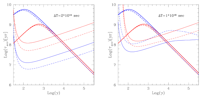
Figure 13: Acceleration time–scales (thin lines) and losses time–scales (thick lines) for relativistic electrons as a function of the Lorentz factor for $2\times 10^{14}$sec (Left Panel) and $10^{16}$sec (Right Panel) from the beginning of the acceleration. Calculations are shown for $n_{th}=3\times 10^{-3}$cm^-3 (red lines) and $n_{th}=10^{-4}$cm^-3 (blue lines), and for $B=0.1\mu$G (solid lines) and $B=1.5\mu$G (dashed lines). In the calculations we assumed: $d(\delta B)^{2}/dt=3.3\times 10^{-15}(\mu{\rm G})^{2}$/s, $T=10^{8}$K, ${\cal E}_{e}=0.001\times{\cal E}_{th}$, ${\cal E}_{p}=0.01\times{\cal E}_{th}$, and $s=2.2$, not specified parameters being those in Fig. 12.

Figure 14: Time evolution of the spectrum of cosmic ray protons as a function of $p$. From bottom to top, the curves are obtained at times $2\times 10^{15}$, $5\times 10^{15}$, $8\times 10^{15}$, $10^{16}$, and $1.5\times 10^{16}$ sec after the beginning of acceleration. The initial proton spectrum is plotted as a dashed line. The values of the parameters are as in Fig. 11.

5 Quasi Stationary Solutions

For a given model for the injection of the waves in the ICM, the spectra of electrons, protons and waves can be calculated using Eqs. (32) with $Q_{e}=0$, (37) and (44). A few comments are in order:

• In this paper we confine our attention to the case of Alfvén waves, that resonate predominantly with relativistic particles. Moreover, we do not consider situations in which the amount of energy injected in the form of turbulence becomes comparable with the thermal energy of the ICM. As a consequence, we can safely assume that the thermal distributions of electrons and protons in the ICM are not appreciably affected by the acceleration processes discussed above.

• The spectra of electrons, protons and waves, as discussed above, result from a coupling between all these components: the spectrum of the waves develops in time due to the turbulent cascade until damping becomes efficient and particle acceleration occurs. It is worth noticing that the time scales for the processes of damping and cascading are quite different from those related to particle losses and transport. While the wave spectrum develops over $\sim 10^{7}$ sec, particle acceleration occurs on time scales of $\geq 10^{14}$sec, and we are interested in following the particle evolution for a typical time of $\geq 10^{15}$sec.

  The clear difference among these time scales suggests that we use a quasi stationary approach, in which it is assumed that at each time-step the spectrum of the waves approaches a stationary solution (obtained by solving Eq. (44) with $\partial W/\partial t=0$) and that this solution changes with time due to the evolution of the spectrum of the accelerated electrons and protons. In other words, at any time-step we solve a set of three differential equations: Eq. (44) (with $\partial W/\partial t=0$), Eq. (37) and Eq. (32). Intermittent injection of turbulence in the ICM may occur on time–scales $\geq 10^{7}-10^{8}$ yrs which are much longer than the time–scales of damping and cascading, and thus the quasi–stationary approach discussed above remains applicable.

5.1 The spectrum of Alfvén Waves

The shape of the spectrum of waves at any time is determined by the damping of these waves, mainly on protons. The proton spectrum in turn changes because of acceleration, and backreacts upon the spectrum of waves: this implies that even for a time-independent rate of injection of waves, the strength of the damping rates and the spectrum of the MHD waves are expected to change with time.

In Fig. 10 we plot an example of the evolution of the time scale for the damping due to relativistic protons: it is clear how the damping rate increases with time, as a consequence of the fact that most of the energy injected in MHD waves is channelled into relativistic protons.

A relevant example of the time evolution of the spectrum of waves is illustrated in Fig. 11: as expected, the energy associated with MHD waves which contribute to the acceleration of the bulk of the relativistic electrons ($k/k_{max}\sim 10^{-1}-10^{-3}$) decreases with time. In addition to the general finding that the spectrum of the Alfvén waves evolves with time, here we also point out that :

• the spectrum is not a simple power law: it has a different slope at different $k$ and the curvature of the spectrum also changes with time;

• the spectrum has a low-$k$ cutoff due to the maximum injection scale, close to the Taylor scale;

• the spectrum has a high-$k$ cutoff generated by the damping with the thermal particles.

5.2 Electron acceleration

The process of electron acceleration via Alfvén waves has been extensively investigated in the literature. Eilek & Henriksen (1984) showed that a self-similar solution for the spectra of electrons and waves can be found if these spectra are both required to be power laws in energy and wavenumber respectively. In this case, the slopes of the electron ($\delta$) and of the waves ($\omega$) spectrum are related by $\delta=6-\omega$.

As pointed out above, the assumption of power law spectra is usually not fulfilled. In fact, more often a stationary solution is found in the form of a pile up spectrum $N(p)\propto p^{2}\exp\{-p/p_{c}\}$ (e.g., Borowsky & Eilek, 1986).

In the general case considered here, the electron spectrum may be even more complex due to the fact that the spectrum of the waves is not a power law and the whole evolution is time-dependent. Note that the initial stage of reacceleration of relic relativistic electrons (i.e. $\gamma\sim 100-1000$ electrons) is mainly affected by the competition between Coulomb losses and acceleration due to the Alfvén waves, while later stages, of further acceleration to the highest allowed energies, are limited by radiative losses.

In Fig. 12 we plot the time scale for electron acceleration, $\sim p^{2}/2D_{pp}$, and compare it with the time scale of the energy losses of electrons for different proton spectra injected in the ICM (see caption). For steep proton spectra, the electron acceleration is more efficient because less energy gets channelled into the proton component. In general, hard proton spectra make the acceleration of electrons to Lorentz factors $\gamma>10^{3}$ relatively difficult.

If this is true in the initial stage of evolution of the system, it becomes increasingly less so at later times: after about $\sim 0.5-0.7$ Gyr, relativistic protons have accumulated enough of the waves energy that the damping of the waves becomes even more efficient and further acceleration of electrons is prevented.

In Fig. 13 we plot the acceleration and cooling time scales of electrons as computed for different values of the density of the ICM and of the magnetic field strength.

It is clear that at the beginning of the reacceleration phase (Fig. 13a) the electron acceleration is enhanced by increasing the magnetic field strength and by decreasing the density of the ICM. On the other hand, at later times in the reacceleration phase, the situation can be much more complicated. In particular, when the reacceleration efficiency is very high (for instance for large values of the magnetic field strength and for low values of $n_{th}$), the energy stored in relativistic protons after few reacceleration times may become sufficiently high to increase the damping rate of the Alfvén waves and thus decrease the efficiency of electron acceleration (Fig. 13b): in this case, higher values of the magnetic field strength produce a lower acceleration efficiency compared with the case of low magnetic field.

The continuous backreaction between waves and protons creates a sort of wave-proton boiler that in a way is self-regulated.

If the injection of fluid turbulence is intermittent on time scales of the order of the cooling time of electrons with Lorentz factors $\gamma\sim 10^{3}-10^{4}$, then the effect of the wave-proton boiler on the electron acceleration may be reduced. The reason for this is that for a given reacceleration rate, the accumulation of energy in the form of relativistic protons requires longer times and the electron acceleration remains efficient for $\sim 1$ Gyr.

5.3 Proton acceleration

Alfvénic acceleration of thermal and relativistic protons is extensively studied in the literature, in particular as applied to the case of solar flares (e.g., Miller, Guessoum, Ramaty 1990; Miller & Roberts 1995).

We consider here the extension of these calculations to the case of Alfvénic acceleration in clusters of galaxies.

If the energy injected in Alfvén waves is significantly larger than that stored by the relativistic protons at the beginning of the acceleration phase, then the spectrum of protons is expected to be considerably modified. Under these conditions, we illustrate, in Fig. 14, the evolution of the spectrum of the relativistic protons. The figure clearly shows that the spectrum flattens and develops a bump.

The prominence of this bump increases with time as the energy absorbed by relativistic protons also increases. Moreover, the bump moves toward larger momenta of the particles during the acceleration time.

The presence of a bump in the proton spectrum may be of some importance in the calculation of the spectrum of the high energy secondary electrons which are expected to be produced during hadronic collisions. We find that, under typical conditions in the ICM and assuming an energetics of the Alfvén waves considerably larger than that of the initial proton population, relevant bumps are produced at energies in excess of $200$ GeV which should be visible in the spectrum of secondary electrons at $\gamma>10^{5}$. We also point out that proton acceleration is strongly reduced at some momentum $p_{max}$ (Fig. 14) which corresponds to the momentum at which the resonance condition [Eq. (15)] is satisfied for wavenumber corresponding to the maximum injection scale of the Alfvén waves [Eq. (39)]. A maximum energy of the injected secondary electrons is expected as well. A detailed discussion of the production of secondary electrons by reaccelerated protons and of their further acceleration will be presented in a forthcoming paper.

A relevant point to make for the process of proton acceleration is to quantify the fraction of the energy injected in Alfvén waves which is absorbed by the relativistic protons and the time needed for relativistic protons to react to the injection of this energy. In Fig. 15, we compare the energy injected in waves with that converted to relativistic protons, for different values of the rates of energy injection in the form of Alfvén waves. After some time, it can be seen that the energy of the protons asymptotically converges to the energy of the waves. It is also clear that there is a delay time between the injection of waves and the proton acceleration, as it is expected due to the finite acceleration time.

5.4 The Wave-Proton Boiler

One of the most important results of our investigation is the quantitative treatment of the backreaction of the accelerated protons on the waves and in turn on the electrons. Qualitatively, given typical conditions in the ICM, we can identify three main temporal stages of the acceleration process:

• Cascading stage:

  For a non negligible rate of energy injection in the form of Alfvén waves, the cascade time is shorter than the damping time. This remains true up to some critical wavenumber, which depends on energetics and spectrum of protons, where damping starts to be relevant. If such a wavenumber is larger than about $10^{-2}k_{max}$, then enough energy is left in the form of waves at the scales which may resonate with relic relativistic electrons. In this case electrons are effectively re-energized.

• Stage of proton backreaction:

  Once the Alfvén waves start to accelerate electrons and protons to higher energies, the spectrum of protons and electrons becomes harder and the fraction of the energy stored in non-thermal particles starts to be large enough to make damping more severe. As a consequence, the rate of electron acceleration is reduced.

• End of acceleration:

  At the beginning of the acceleration phase, the bulk of protons is located at supra-thermal or trans-relativistic energies. It takes a few $10^{8}$yrs, however, for these protons to be energized to higher energies, as illustrated in Fig. 16, where we plot the acceleration time scale of relativistic protons (we chose a relatively steep injection spectrum). From Fig. 16 we see that after about $0.5-0.7$ Gyr the acceleration time scale has increased by about one order of magnitude. At this point the acceleration stage of protons and electrons can be considered as concluded, unless the injection of turbulence occurs intermittently (see Sect.5.2).

  After the end of the third stage, the electrons cool due to radiative and Coulomb losses, while the Alfvén acceleration is only able to prevent the thermalization of these particles maintaining their Lorentz factor around $\gamma\sim 100-1000$.

Figure 15: Evolution of the energy density stored in the form of cosmic ray protons ($p>0.1\,m_{p}c$) as a function of time from the beginning of the acceleration stage for three different injection rates of Alfvén waves: $d(\delta B)^{2}/dt=3.3\times 10^{-15}$ (points-solid line), $1.9\times 10^{-15}$ (points-dotted line), and $8.2\times 10^{-16}(\mu{\rm G})^{2}$/s (points-dashed line). For comparison the energy density injected in Alfvén waves is aslo plotted. In the calculations we assume the following values of the parameters: $B=0.5\mu$G, $T=10^{8}$K, $n_{th}=10^{-3}$cm^-3, ${\cal E}_{e}=0.001\times{\cal E}_{th}$, ${\cal E}_{p}=0.01\times{\cal E}_{th}$, $s=2.2$ and $z_{i}=1.0$.

Figure 16: Evolution of the proton acceleration time–scale during the acceleration phase as a function of $p$. From bottom to top the curves refer to $2\times 10^{15}$, $5\times 10^{15}$, $10^{16}$, and $2\times 10^{16}$ sec after the beginning of the acceleration stage. The following values of the parameters have been adopted: $d(\delta B)^{2}/dt=3.3\times 10^{-15}(\mu{\rm G})^{2}$/2, $B=0.5\mu$G, $T=10^{8}$K, $n_{th}=10^{-3}$cm^-3, ${\cal E}_{e}=0.001\times{\cal E}_{th}$, ${\cal E}_{p}=0.0025\times{\cal E}_{th}$ and $s=3.0$.

6 Non-thermal emission from galaxy clusters

6.1 Cluster mergers and turbulence

Major mergers are among the most energetic events in the Universe. Cluster mergers involve a collision of at least two subclusters with relative velocity of $\sim 1000-2000$ km s^-1. During these events, a gravitational energy in excess of $10^{63}$ erg is released through the formation of shock waves. Numerical simulations show that cluster mergers can generate relatively strong turbulence in the ICM (Norman & Bryan 1999; Roettiger et al., 1999; Ricker & Sarazin 2001). The bulk of the turbulence is most likely injected on scales $\geq 100$ kpc during the motion of the subclusters. Afterwards this turbulence eventually cascades toward smaller scales. As discussed in Sect.3.1, when the turbulent cascade reaches scales close to the Taylor scale, a fraction of the energy flux of the fluid turbulence can be transferred to MHD waves which in turn can accelerate fast particles.

For simplicity, we assume here that the bulk of the fluid turbulence in a given point of the cluster volume is injected at the scale $l_{o}$, for a time $\tau_{i}$, of the order of the time necessary for the subclump to cross the scale $l_{o}$:

$$\tau_{i}({\rm Gyr})\sim 0.3\xi\Big{(}{{l_{o}}\over{300}}\Big{)}\Big{(}{{v_{c}}\over{10^{3}}}\Big{)}^{-1},$$ (63)

where $v_{c}$ is the velocity of the subclump in the host cluster and $\xi$ is a parameter of the order of a few. Within these assumptions, the injection rate of energy in the form of fluid turbulence is given by :

$$F_{f}\sim{{2.3\times 10^{-27}}\over{\xi}}\Big{(}{{n_{\rm th}}\over{10^{-3}}}\Big{)}\Big{(}{{T}\over{10^{8}}}\Big{)}\Big{(}{{l_{o}}\over{300}}\Big{)}^{-1}\Big{(}{{v_{c}}\over{10^{3}}}\Big{)}{{{\cal E}_{t}}\over{{\cal E}_{th}}},$$ (64)

where ${\cal E}_{\rm th}$ is the local energy density of the ICM in the form of thermal gas and ${\cal E}_{\rm t}$ is that in the form of turbulence. The bulk of the fluid turbulence at the scale $l_{o}$ then cascades toward smaller scales producing a spectrum of the fluid turbulence that we write as $W_{f}(x)\propto x^{-m}$ (Sect. 3.1). Assuming a Kolmogorov phenomenology for the wave-wave diffusion in $k-$space, the time scale for the cascade can be estimated from Eq. (62) with $I_{x_{o}}\sim x_{o}^{-1}F_{f}$:

$$\tau_{s}({\rm Gyr})\sim 0.2\Big{(}{{l_{o}}\over{300}}\Big{)}\Big{(}{{10^{8}}\over{T}}\Big{)}^{1/3}\Big{(}{{10^{3}}\over{v_{c}}}\Big{)}^{1/3}\xi^{1/3}\Big{(}{{0.1}\over{{\cal E}_{t}/{\cal E}_{th}}}\Big{)}^{1/3}.$$ (65)

In our simple approach, this is the time delay between the merger event and the development of the turbulence at small scales (and thus the production of MHD waves). In the case of Alfvén waves in the framework of a Kolmogorov phenomenology, the power injected in waves is [Eq. (49)]:

$$P_{A}=\int I(k)dk\simeq\,\,\,\,\,\,\,\,\,\,\,\,\,\,\,\,\,\,\,\,\,\,\,\,\,\,\,\,\,\,\,\,\,\,\,\,\,\,\,\,\,\,\,\,\,\,\,\,\,\,\,\,\,\,\,\,\,\,\,\,\,\,\,\,\,\,\,\,\,\,\,\,\,\,\,\,\,\,\,\,\,\,\,\,\,\,\,\,\,\,$$

$${{1.5\times 10^{-29}}\over{{{\cal R}_{16}}^{{1\over 6}}}}\Big{(}{{v_{\rm f}}\over{400}}\Big{)}^{4}B_{\mu G}^{-1}\Big{(}{{n_{\rm th}}\over{10^{-3}}}\Big{)}^{{3\over 2}}\Big{(}{{l_{o}}\over{300}}\Big{)}^{-1}$$ (66)

All the quantities involved in the calculation of the power radiated in the form of Alfvén waves can be relatively well modelled. The only parameter which is very difficult to estimate is the value of the Reynolds number, ${\cal R}=l_{o}v_{f}/\nu_{K}$, due to the large uncertainties in the value of the kinetic viscosity $\nu_{K}=u_{p}\lambda_{eff}/3$ ($u_{p}$ is the thermal velocity and $\lambda_{eff}$ the effective mean free path of protons). For transverse drift of protons in a magnetic field $B$, the mean free path is given by $\lambda_{eff}\sim\lambda_{g}^{2}/\lambda_{c}$ (e.g., Spitzer 1962) with $\lambda_{g}$ and $\lambda_{c}$ being the proton gyroradius and the mean free path due to Coulomb collisions respectively. In this case the kinetic viscosity is given by (Fujita et al. 2003, and references therein):

$$\nu_{K}=1.3\times 10^{5}\Big{(}{{n_{th}}\over{10^{-3}}}\Big{)}\Big{(}{{T}\over{10^{8}}}\Big{)}^{-1/2}\Big{(}{{\ln\Lambda}\over{40}}\Big{)}B_{\mu G}^{-2}.$$ (67)

The resulting Reynolds number is:

$${\cal R}\sim 2.8\times 10^{26}\Big{(}{{l_{o}}\over{300}}\Big{)}\Big{(}{{v_{f}}\over{400}}\Big{)}\Big{(}{{10^{-3}}\over{n_{th}}}\Big{)}\Big{(}{{T}\over{10^{8}}}\Big{)}^{{1\over 2}}B_{\mu G}^{2}\Big{(}{{40}\over{\ln\Lambda}}\Big{)},$$ (68)

which is extremely large and, most likely, should be considered as an upper limit, due to the assumption of transverse drift of protons on the magnetic field lines. In general, diffusion of the protons along the magnetic field lines can substantially increase the value of $\lambda_{eff}$ and thus reduce ${\cal R}$. The Reynolds number has been roughly estimated in a number of astrophysical situations, being $\sim 10^{7}$ in the solar wind (e.g., Grappin et al 1982), $\sim 10^{11}$ in the extragalactic radio jets imaged with the VLA (e.g., Henriksen, Bridle, Chan 1982), $\sim 10^{14}$ in the solar corona (e.g., Ofman & Aschwanden, 2002) and $\sim 10^{16}$ for the hot phase of the local interstellar medium (e.g., Armstrong, Rickett, Cordes 1981). Following this last estimate, in our modelling we take ${\cal R}\sim 10^{16}$ but also stress that, due to the poor dependence of $P_{A}$ on ${\cal R}$, an uncertainty in ${\cal R}$ by six orders of magnitude implies only one order of magnitude change in $P_{A}$.

In our simple model for the merger, it is easy to show that the condition $P_{A}<<F_{f}$ is satisfied, therefore the application of the Lightill scheme in our calculations appears to be self-consistent.

The power radiated in the form of Alfvén waves strongly depends on the velocity of the eddies in the fluid turbulence. In addition, assuming that the energy of the fluid turbulence is a fraction of the local thermal energy (i.e., ${\cal E}_{t}\sim\rho v_{f}^{2}$, and $v_{f}$=const) and that the largest scale of the spectrum of turbulence, $l_{o}$, does not depend on the position in the cluster volume, we notice that the injected power in Alfvén waves increases with increasing the number density of the ICM and with decreasing the strength of the local magnetic field. For instance, assuming a typical scaling law for the magnetic field in the cluster $B\propto n_{\rm th}^{2/3}$, it would be $P_{A}\propto n_{\rm th}^{5/6}$, namely the power injected in the form of Alfvén waves is expected to be slightly larger in the central regions of the cluster.

A second important quantity in our calculations is the largest scale of the spectrum of the Alfvén waves, $k_{T}\sim x_{T}v_{f}(x_{T})/v_{A}$. It is convenient to parametrize this quantity in terms of the wavenumber corresponding to the minimum scale of the MHD waves, $k_{max}\sim\Omega_{p}/v_{M}$, namely:

$${{k_{T}}\over{k_{\rm max}}}\simeq{{{{\cal R}_{16}}^{{1\over 3}}}\over{2.4\cdot 10^{7}}}\Big{(}{{n_{\rm th}}\over{10^{-3}}}\Big{)}^{{1\over 2}}\Big{(}{{300}\over{l_{o}}}\Big{)}B_{\mu G}^{-2}\Big{(}{{v_{\rm f}}\over{400}}\Big{)}\Big{(}{{T}\over{10^{8}}}\Big{)}^{{1\over 2}}.$$ (69)

Given the resonance condition [Eqs.(27) and (35)], the presence of a maximum scale in the wave spectrum, $l_{T}\sim 2\pi/k_{T}$, implies a limit for the energy of the particles that can be efficiently accelerated:

$${\cal E}_{res}({\rm TeV})\leq 24\times\Big{(}{{k_{max}/k_{T}}\over{6\cdot 10^{6}}}\Big{)}\Big{(}{{T}\over{10^{8}}}\Big{)}^{1/2}$$

$$\propto{\cal R}^{-1/3}n_{th}^{-1/2}l_{o}B^{2}{v_{f}}^{-1}.$$ (70)

This limit provides a relatively good estimate in the case of relativistic protons, which are basically loss-free particles, while the maximum energy of the electrons is driven by the competition between acceleration and loss terms.

Figure 17: Maximum energy attainable for relativistic electrons during the acceleration (only systematic terms are considered here) plotted as a function of $\Psi$. Left Panel: $\gamma_{\rm max}$ at $3\times 10^{15}$ (dashed line) and $10^{16}$sec (solid line) after the beginning of the acceleration stage. The values of the parameters are: $B=1\mu$G, $n_{th}=10^{-3}$cm^-3, ${\cal E}_{e}=0.001\times{\cal E}_{th}$, ${\cal E}_{p}=0.003\times{\cal E}_{th}$, $s=2.2$, and $z_{i}=1.0$. Right Panel: $\gamma_{\rm max}$ at $10^{16}$sec from the beginning of the acceleration stage for ${\cal E}_{p}=0.003\times{\cal E}_{th}$ (solid line) and ${\cal E}_{p}=0.03\times{\cal E}_{th}$ (dashed line). Other parameters are as in the Left Panel case.

6.2 Constraining the model parameters

In this Section we derive some constraints on the physical conditions in the ICM in order to obtain the reacceleration efficiency necessary to allow the production of the observed non–thermal emission.

From Eq. (66) it is clear that a key parameter in the calculation of the efficiency of particle acceleration in our approach is given by :

$$\Psi=\Big{(}{{v_{f}}\over{400}}\Big{)}^{4}\Big{(}{{{\cal R}}\over{10^{16}}}\Big{)}^{-1/6}\Big{(}{{l_{o}}\over{300}}\Big{)}^{-1},$$ (71)

which is very sensitive to the velocity of the eddies in the fluid turbulence. A constraint on this velocity can be obtained by requiring that the energy injected in the form of fluid turbulence (${\cal E}_{t}\sim x_{o}W(x_{o})\sim m_{p}n_{th}v_{f}^{2}$) does not exceed the thermal energy. From Eqs. (63) and (64) we obtain:

$$\Big{(}{{v_{f}}\over{400}}\Big{)}\leq 3\Big{(}{{T}\over{10^{8}}}\Big{)}^{1/2}\Big{(}{{{\cal E}_{t}}\over{{\cal E}_{th}}}\Big{)}^{1/2}.$$ (72)

An additional constraint to the parameter $\Psi$ comes from requiring that the energy stored in the form of relativistic protons is small enough to allow for efficient electron acceleration.

As pointed out above, after an acceleration time of the order of 0.5-0.7 Gyr, relativistic protons get a large fraction of the energy previously in the form of Alfvén waves. We limit ourselves to cases in which $P_{A}\cdot\tau_{i}<0.1\,{\cal E}_{th}$. From Eqs. (63) and (66) one has:

$$\Psi\leq{{16}\over{\xi}}B_{\mu G}\Big{(}{{n_{th}}\over{10^{-3}}}\Big{)}^{-{1\over 2}}\Big{(}{{T}\over{10^{8}}}\Big{)}\Big{(}{{l_{o}}\over{300}}\Big{)}^{-1}.$$ (73)

Finally, we are interested in the production of relatively long-living (e.g., for $>0.3$ Gyr) non-thermal phenomena, in order to have a chance of observing them in some clusters. From Eq. (63) we can set a limit on the parameter $\xi$:

$$\xi>\Big{(}{{v_{c}}\over{1000}}\Big{)}\Big{(}{{l_{o}}\over{300}}\Big{)}^{-1}.$$ (74)

The maximum energy, $\gamma_{max}$, of the accelerated electrons is obtained by balancing energy losses and energy gains.

In Fig. 17a we plot $\gamma_{max}$ as a function of $\Psi$, for different acceleration times, $\Delta T$, for a given set of values of the parameters defining the environment of cluster cores. In Fig. 17b we plot the same quantity for different values of the energy density in the form of relativistic protons, ${\cal E}_{p}$. The injection spectrum of protons is taken as a power law with slope 2.2.

In order to obtain $\gamma_{max}>>1000$, needed to explain the synchrotron emission at GHz frequency as well as the IC hard X–ray photons, we are forced to require that $\Psi\geq 1$ and ${\cal E}_{p}\leq 3\%\,{\cal E}_{th}$.

Such a stringent limit is the consequence of the effective damping of Alfvén waves upon the relativistic proton component, which inhibits the acceleration of electrons.

In the periphery of the cluster, where the magnetic field is expected to be lower, the conditions to obtain high energy electrons are less stringent. It remains true however that no more than a few percent of the thermal energy of the cluster can be in the form of relativistic protons if we want to interpret the observed non-thermal phenomena as the result of radiative processes of high energy electrons accelerated via Alfvén waves.

A steeper injection spectrum of protons, containing the same energy density, makes the constraints found above even more stringent; however this would imply a very large energy injected in relativistic protons in the ICM.

On the other hand, at given proton number density, a steeper spectrum contains less relativistic particles, which would allow for more efficient electron acceleration.

Figure 18: Synchrotron cut–off frequency as a function of the magnetic field strength in the case of $n_{\rm th}=10^{-3}cm^{-3}$ (empty symbols) and $n_{\rm th}=2\times 10^{-4}cm^{-3}$ (filled symbols). The results are reported after $7\times 10^{15}$sec of reacceleration. In the calculations the following values of the parameters have been used: $d(\delta B)^{2}/dt=3.3\times 10^{-15}(\mu{\rm G})^{2}$/s, $T=10^{8}$K, ${\cal E}_{e}=0.001\times{\cal E}_{th}$, ${\cal E}_{p}=0.01\times{\cal E}_{th}$, $s=2.2$ and $z_{i}=1.0$.

Clearly, a crucial parameter in the modeling of the non–thermal phenomena in galaxy clusters is the strength of the magnetic field in the ICM. There is still debate on whether this field is of several $\mu G$ or rather fractions of $\mu G$: on one hand, if the hard X–ray excess is interpreted as a result of IC emission of relativistic electrons, the required volume averaged field is $\leq 0.2-0.4\mu$G (e.g. Fusco–Femiano et al. 2002). On the other hand, Faraday rotation measurements (RM) of the radiation coming from cluster radio sources seem to require a magnetic field strength of $\sim 4-8\mu$G (e.g., Clarke et al. 2001). A number of possibilities to reconcile these two predictions have been proposed in the literature, based on either choosing more realistic spectra of the radiating particles or introducing a spatial distribution of non-thermal particles and magnetic fields (Goldshmidt & Rephaeli 1993; Brunetti et al. 2001a; Petrosian 2001; Kuo et al. 2003).

It is also worth recalling that Faraday RM do not provide a direct measurement of the magnetic field, but rather an estimate of a quantity which is a (not necessarily trivial, e.g. Clarke 2002) convolution of the component of the magnetic field parallel to the line of sight, of the electron density and that accounts for the topology of the magnetic field: Newman et al. (2002) showed how the assumption of a single–scale magnetic field leads to an overestimate of the field strength extracted from RM. Other authors have further discussed the influence of the power spectrum of the magnetic field topology in the ICM on the RM (Ensslin & Vogt 2003; Vogt & Ensslin 2003; Govoni et al. 2003).

In order to illustrate the effect of these uncertainties on the conclusions inferred from our calculations, we evaluated the so-called synchrotron cut–off frequency for a cluster with temperature $T=10^{8}$ K and with a relic electron and proton energy densities chosen as ${\cal E}_{e}=0.001\times{\cal E}_{th}$, ${\cal E}_{p}=0.01\times{\cal E}_{th}$ (protons have a spectrum with power index $s=2.2$; see caption of Fig. 18 for additional information). The calculation is carried out for a dense region ($n_{\rm th}=10^{-3}cm^{-3}$ [empty symbols]) and for a low density region ($n_{\rm th}=2\times 10^{-4}cm^{-3}$ [filled symbols]). Given the shape of the spectrum of the accelerated electrons, a synchrotron cut–off at $\geq 300$ MHz is required to account for the synchrotron radiation observed in the form of radio halos.

Our conclusion, based on Fig. 18, is that in high density regions ($n_{\rm th}\sim 10^{-3}$cm^-3) Alfvénic reacceleration of relic electrons cannot be an efficient process for $B\gg 4\mu$G and for $B\ll 0.5\mu$G. These constraints become less stringent in the case of low density regions.

6.3 A simplified models for Radio Halos and Hard X–ray emission

The best evidence for the diffuse non-thermal activity in clusters of galaxies is provided by the extended synchrotron radio emission observed in about $\sim 30$ massive clusters of galaxies (e.g., Feretti, 2002). A recent additional evidence supporting the existence of relativistic electrons is given by the hard X–ray tails in excess to the thermal emission discovered by BeppoSAX and RXTE in the case of a few galaxy clusters (e.g., Fusco-Femiano et al. 2002). The possibility that hard X–ray tails are due to IC scattering of the CMB photons is intriguing as, in this case, radio and HXR radiations would be emitted by roughly the same electron population and thus the combination of radio and HXR data would allow us to infer an estimate of the volume-averaged magnetic field strength and of the energy density of relativistic electrons. Additional pieces of evidence for non–thermal phenomena are the so called radio Relics and the EUV excesses whose origin may however be not directly connected to that of radio halos and HXR. Therefore these phenomena will not be modelled in the present paper. For a recent review on these arguments the reader is referred to Ensslin (2002, and ref. therein) and Bowyer (2002, and ref. therein).

In this section we apply the formalism described in previous sections in order to show that for the conditions realized in the ICM, Alfvénic reacceleration of relic electrons may generate the observed radiation, provided the energy content in the form of relativistic protons is not too large. For simplicity we neglect here the production and reacceleration of secondary products of proton interactions.

Figure 19: Temporal evolution of the accelerated electron spectra after 0, $10^{14}$, …, $5\times 10^{15}$, $7\times 10^{15}$, $10^{16}$, and $1.2\times 10^{16}$sec from the beginning of the acceleration stage. The following values of the parameters have been used: $d(\delta B)^{2}/dt=1.6\times 10^{-15}(\mu{\rm G})^{2}$/s, $B=0.5\mu$G, $T=10^{8}$K, $n_{th}=10^{-3}$cm^-3, ${\cal E}_{e}=0.001\times{\cal E}_{th}$, ${\cal E}_{p}=0.01\times{\cal E}_{th}$, $s=2.2$ and $z_{i}=1.0$.

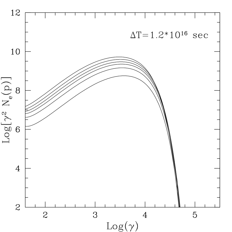
Figure 20: Spectra of electrons accelerated for $1.2\times 10^{16}$sec at different distances from the cluster center: $r=$0.3, 0.6, 0.9, 1.2, 1.4, 2.1$r_{\rm c}$ (from top of the diagram). The central values assumed in the calculations are : $n_{th}(0)=1.5\times 10^{-3}$cm^-3, $B(0)=1.5\mu$G, $d(\delta B(0))^{2}/dt=2.2\times 10^{-15}(\mu{\rm G})^{2}$/s with the scaling laws given in Sect. 6.3, $r_{\rm c}=400$ kpc.

Figure 21: Temporal evolution of the synchrotron (Left Panel) and ICS (Right Panel) spectra from the cluster model given in Sect. 6.3 (integrating the emissivities up to $5\times r_{c}$). Spectra are shown at $5\times 10^{15}$, $1.2\times 10^{16}$ and $1.7\times 10^{16}$sec from the beginning of the acceleration (from bottom to top). In the calculations ${\cal E}_{e}=5\times 10^{-5}{\cal E}_{th}$ has been adopted. Radio data are taken from Thierbach et al. (2003), EUV from Bowyer et al. (1999; here reported as an upper limit, see text), XHR from Fusco–Femiano et al. (2004).

Our simple model for the ICM assumes a $\beta$-model (Cavaliere & Fusco-Femiano, 1976) for the radial density profile of the thermal gas in the ICM, in the form

$$n_{th}(r)=n_{th}(r=0)\Big{(}1+({{r}\over{r_{c}}})^{2}\Big{)}^{-3\beta/2},$$ (75)

where $r_{c}$ is the core radius and we adopted $\beta=0.8$. The magnetic field is assumed to scale with density according with flux conservation:

$$B(r)=B(r=0)\Big{(}{{n_{th}(r)}\over{n_{th}(r=0)}}\Big{)}^{2/3}.$$ (76)

Based on the constraints given in Sect. 6.2 we adopt $B(r=0)\sim 0.5-4\mu$G.

Finally, we assume that the ratio between the energy density of the relic relativistic particles (at the beginning of the acceleration phase) and that of the thermal plasma is constant with distance throughout the cluster volume:

$${\cal E}_{p[e]}={\cal E}_{th}\eta_{p[e]},$$ (77)

where $\eta_{p[e]}$ is a free parameter ($\eta<0.1$).

For simplicity we also assume that the maximum injection scale of the turbulence, the Reynolds number and the velocity of the turbulent eddies are independent of the location within the cluster volume.

Using the scaling relationship for the magnetic field, Eq. (76), and the expression for the injection power in the form of Alfvén waves, Eq. (66), we obtain:

$$P_{A}(r)=P_{A}(r=0)\Big{(}{{n_{th}(r)}\over{n_{th}(r=0)}}\Big{)}^{5/6}.$$ (78)

The spectrum of the relativistic electrons in the core region is plotted in Fig. 19. We can see that the bulk of relativistic electrons, initially at $\gamma\sim 10^{2}$, can be energized up to $\gamma\sim 10^{4}$ for a relatively long time.

Eq. (78) indicates that, in our simple approach, the power injected in the form of Alfvén waves decreases with increasing distance from the cluster center. Since radio halos have a considerable size, it is needed to check that our model provides enough energy in the outskirts of clusters.

In Fig. 20 we plot the electron spectra at different distances from the cluster center (see caption). What emerges from this figure is that at large distances the effect of acceleration is even stronger than in the central region and the electron spectra peak at slightly higher energies than in the core. This is due to the fact that in the outskirts the damping rate is reduced more than the rate of injection of turbulence.

The synchrotron emissivity roughly scales as $J_{syn}\propto N_{e}\gamma_{max}(r)^{2}B^{2}\propto n_{th}^{7/3}\gamma_{max}(r)^{2}$. Such a relatively soft dependence of the emissivity on the radius allows for a relatively broad synchrotron brightness profile.

More specifically, the synchrotron emissivity can be written as:

$$J_{syn}(\nu,t)={{\sqrt{3}e^{3}B}\over{mc^{2}}}\int_{p}\int_{0}^{{\pi}\over 2}dpd\theta\sin^{2}\theta N(p,t)F\Big{(}{{\nu}\over{\nu_{c}}}\Big{)},$$ (79)

where the synchrotron Kernel is given by (e.g., Rybicki & Lightman, 1979):

$$F\Big{(}{{\nu}\over{\nu_{c}}}\Big{)}={{\nu}\over{\nu_{c}}}\int_{\nu/\nu_{c}}^{\infty}K_{5\over 3}(y)dy,$$ (80)

and $\nu_{c}=(3/4\pi)p^{2}eB\sin\theta/(mc)^{3}$.

The emissivity due to inverse Compton scattering off the CMB photons is given by (Blumenthal & Gould, 1970):

$$J_{ic}(\nu_{1},t)=\Big{(}2\pi r_{o}m^{2}c\Big{)}^{2}h\nu_{1}^{2}\int_{\nu}\int_{p}d\nu dp{{N(p,t)p^{-4}}\over{\exp({{h\nu}\over{k_{B}T_{z}}})-1}}\times$$

$$\Big{(}1+2\ln\Big{(}{{\nu_{1}m^{2}c^{2}}\over{4p^{2}\nu}}\Big{)}+{{4p^{2}\nu}\over{m^{2}c^{2}\nu_{1}}}-{{m^{2}c^{2}\nu_{1}}\over{2p^{2}\nu}}\Big{)},$$ (81)

where $T_{z}=2.73(1+z)$ is the temperature of the CMB photons.

The corresponding synchrotron and IC spectra are plotted in Fig. 21 at different times, for a central magnetic field $B(r=0)\simeq 1\mu G$. The spectra are compared with that observed for the radio halo in the Coma cluster : an initial energy density in the relic relativistic electrons of the order of $5\times 10^{-5}{\cal E}_{th}$ is required to account for the data. In Fig. 21 we also report the luminosity of the EUV excess in the Coma cluster as an upper limit since it is commonly accepted that the origin of the EUV excess is not directly related to the same electron population responsible for the radio and possibly for the HXR emission (Bowyer & Berghöfer 1998; Ensslin et al. 1999; Atoyan & Völk 2000; Brunetti et al. 2001b; Tsay et al. 2002). Here we stress that Fig. 21 does not show the best fit to the data but just a comparison between data and time evolution of the emitted spectra resulting from the very simple scaling of the parameters described above. On the other hand, it should also be stressed that the time evolution of the synchrotron and IC spectra reported in Fig. 21 is generated via the first fully self-consistent calculation of particle acceleration in galaxy clusters. Thus provided that the energy of relativistic protons in galaxy clusters is not larger than a few percent of the thermal energy, Fig. 21 proves, the possibility to obtain the observed magnitude of the non–thermal emission in these objects via Alfvénic acceleration.

In passing we note that the integrated radio spectrum at $\sim$ GHz frequencies is steeper than the IC spectrum in the hard X–ray band independently of the time slice. This seems in nice agreement with some temptative evidences published in some recent literature (Fusco-Femiano et al., 2000; 2002).

7 Conclusions

The origin of the extended non-thermal emission in galaxy clusters is still a subject of active investigation. Despite the numerous models put forward to explain the observed features of this diffuse emission, only some of them appear to be able to describe the observations in detail. One of the approaches that has definitely produced the most promising results consists in the continuous reacceleration of relic relativistic electrons leftover of the past activity occurred within the ICM. The reacceleration is likely to occur through resonant interaction of electrons and MHD waves.

In this paper we presented a full account of the time-dependent injection of fluid turbulence, its cascade to smaller scales, the radiation of Alfvén waves through the Lighthill mechanism, the resonant interaction of these waves with electrons and protons (namely their acceleration) and the backreaction of the accelerated particles on the waves.

The solution of the coupled evolution equations for the electrons, protons and waves revealed several new interesting effects resulting from the interaction among all these components:

i) Alfvén waves are radiated by the fluid turbulence through the Lighthill mechanism. This allows us to establish a direct connection between the fluid turbulence likely to be excited during cluster mergers, and the MHD turbulence that may resonate with particles in the ICM.

ii) Previous calculations looked for self-similar solutions for the spectra of electrons and MHD waves in the form of power laws. The solutions obtained in the present paper show that in Nature these self-similar solutions are not necessarily achieved. In general the system evolves toward complex spectra of electrons and MHD waves with a bump in the electron spectrum, that moves in time toward an increasingly large particle momentum.

iii) We limit ourselves here with the case of Alfvén waves, which couple efficiently with both thermal and relativistic protons, but only with relativistic electrons. The main damping of Alfvén waves occurs on relativistic protons, if there are enough of them. The spectrum of the waves is cutoff at small scales due to the damping of these waves. The damping moves energy from the waves to the particles, determining their acceleration/heating.

iv) The importance of the presence of the relativistic protons for the acceleration of electrons is one of the most relevant new results of this work. A large fraction of the thermal energy in the form of relativistic protons enhances the damping rates of Alfvén waves, suppressing the possibility of resonant interaction of these waves with electrons. Since electrons are the particles that radiate the most, a too large fraction of relativistic protons suppresses non-thermal phenomena directly related to electron reacceleration via Alfvén resonance. It is worth reminding that in principle the secondary electrons and positrons resulting from hadronic interactions may also be re-energized by waves. We neglect this effect here. Our results show that no more than a few percent of the thermal energy density of the cluster can be in the form of relativistic protons if we want to interpret the diffuse radio and hard X-ray emissions as the result of synchrotron and ICS radiation of relic electrons reaccelerated through Alfvén waves. This appears as a stringent constraint on the combination of proton number and spectrum since the accumulation of large number of protons in the ICM is predicted by both analytical calculations (Berezinsky, Blasi & Ptuskin 1997) and numerical simulations (Ryu et al. 2003). The amount of energy piled up in the form of protons in the ICM depends strongly upon the history of cosmic ray injection: the ICM is polluted with cosmic ray protons both due to single sources such as galaxies, radio galaxies and active galaxies, but also due to diffuse acceleration events, such as mergers of clusters of galaxies and accretion of cosmological gas onto a gravitational potential well of a cluster which has already been formed. The spectrum of the cosmic rays diffusively trapped in the ICM depends upon their origin. It is expected that mergers may contribute a major fraction of these cosmic rays, but the spectrum has been calculated to be relatively steep because of the weakness of the merger related shocks. Accretion on the other hand, contributes spectra which are as flat as $E^{-2}$. Both the energy and spectrum of the cosmic rays stored in the ICM affect the temporal evolution of Alfvén waves and their ability to reaccelerate relic electrons. If future observations will unveil the presence of a population of relativistic protons in the ICM with $>5-10$% of the thermal energy, then Alfvénic reacceleration of relativistic electrons in galaxy clusters will be discarded as a possible explanation of non-thermal phenomena in the ICM. On the other hand, similar reacceleration phenomena can be driven by MHD waves other than Alfvén waves (e.g., MS, LH), for which the energy transfer does not occur preferentially toward protons. In this case, the bounds presented here on the allowed energy density in the form of relativistic protons in the ICM could be substantially relaxed.

v) By assuming that protons have a relatively flat spectrum ($s\sim 2.2$) and that they contain up to a few percent of the thermal energy, we used a simple but phenomenologically well motivated model for the density and magnetic field in a cluster of galaxies in order to calculate the expected non-thermal radio and hard X-ray activity of the cluster as a function of time. For the first time we performed a fully self consistent calculation and showed that the reacceleration of relic electrons through resonant interaction with Alfvén waves can explain very well the observed phenomena, including the extended diffuse appearance of this emission. In passing, without considering the case of the HXR emission, we also showed that a magnetic field strength in the range $0.5-4\mu$G in the cluster cores allow electron acceleration efficient enough to produce GHz synchrotron emission. These conditions are less stringent in the outermost regions of the clusters.

vi) In our calculations we adopted a constant injection rate of turbulence during particle acceleration. In this case, even assuming ${\cal E}_{p}<0.1\times{\cal E}_{th}$, we find that after a few $10^{8}$yrs of acceleration the backreaction of protons on MHD waves can suppress the acceleration of energetic electrons : this provides a limit on the duration of the non-thermal phenomena in galaxy clusters. It is possible to extend the duration of non-thermal activity assuming that injection of turbulence occurs in relatively short bursts of duration comparable with the life–time of electrons. On the other hand, independently on the assumptions, our results show that if particle acceleration is mainly due to Alfvén waves, then the existence of radio halos and HXR tails in massive clusters should be limited to achieve periods of $<10$% of the Hubble time.

vii) The temporal duration of the process of turbulent cascade, and the acceleration time scale of electrons are estimated to be about one order of magnitude shorter than the dynamical time-scale of a merger event. This implies that a temporal correlation is still expected between merging processes and the rise of the non-thermal phenomena in galaxy clusters.

8 Acknowledgements

We thank L. Feretti and G. Setti for useful discussions and an anonymous referee for useful comments on the manuscript. G.B. and R.C. acknowledge partial support from CNR grant CNRG00CF0A. The research activity of P.B. and S.G. is partially funded through grants Cofin-2002 and Cofin-2003.

References

- [1] Armstrong J.W., Rickett B.J., Cordes J.M., 1981, Nature 291, 561
- [2] Atoyan A.M., Völk H.J., 2000, ApJ 535, 45
- [3] Barnes A., Scargle J.D., 1973, ApJ 184, 251
- [4] Berezinsky V.S., Blasi P., Ptuskin V.S., 1997, ApJ 487, 529
- [5] Berghöfer T.W., Bowyer S., Korpela E., 2000, ApJ 535, 615
- [6] Berrington R.C., Dermer C.D., 2003, ApJ 594, 709
- [7] Biermann P.L., Ensslin T.A., Kang H., Lee H., Ryu D., 2002, in ’Matter and Energy in Clusters of Galaxis’, ASP Conf. Series, 301, p.293, eds. S. Bowyer and C.-Y. Hwang
- [8] Blandford R., Eichler D., 1987, PhR 154, 1B
- [9] Blasi P., 2000, ApJ 532, L9
- [10] Blasi P., 2001, APh 15, 223
- [11] Blasi P., Colafrancesco S., 1999, APh 12, 169
- [12] Blumenthal G.R.; Gould R.J., Rev of Mod Phys. 42, 237
- [13] Bonamente M., Lieu R, Mittaz J, 2001, ApJ 547, L7
- [14] Borovsky J.E., Eilek J.A., 1986, ApJ 308, 929
- [15] Bowyer S., 2002, in ’Matter and Energy in Clusters of Galaxis’, ASP Conf. Series, 301, p.125, eds. S. Bowyer and C.-Y. Hwang
- [16] Bowyer S., Lampton M., Lieu R., 1996, Science 274, 1338
- [17] Bowyer S., Berghöfer T., 1998, ApJ 506, 502
- [18] Bowyer S., Berghöfer T., Korpela E., 1999, ApJ 526, 592
- [19] Brunetti G., 2002, in ’Matter and Energy in Clusters of Galaxis’, ASP Conf. Series, 301, p.349, eds. S. Bowyer and C.-Y. Hwang
- [20] Brunetti G., Setti G., Feretti L., Giovannini G., 2001a, MNRAS 320, 365
- [21] Brunetti G., Setti G., Feretti L., Giovannini G., 2001b, New Astronomy 6, 1
- [22] Carilli C.L., Taylor G.B., 2002, A&AR 40, 319
- [23] Cavaliere A., Fusco-Femiano R., 1976, A&A 49, 137
- [24] Clarke T.E., 2002, in ’Matter and Energy in Clusters of Galaxis’, ASP Conf. Series, 301, p.185, eds. S. Bowyer and C.-Y. Hwang
- [25] Clarke T.E., Kronberg P.P., Böhringer H., 2001 ApJ 547, L111
- [26] Dennison B., 1980, ApJ 239, L93
- [27] De Young D.S., 1980, ApJ 241, 81
- [28] Dogiel V.A., 2000, A&A 357, 66
- [29] Drury L., 1983, RPPh 46, 973
- [30] Eilek J.A., 1979, ApJ 230, 373
- [31] Eilek J.A., Henriksen R.N., 1984, ApJ 277, 820
- [32] Eilek J.A., Weatherall J.C., 1999, in ’Diffuse Thermal and Relativistic Plasma in Galaxy Clusters’, MPE Report 271, eds. H. Böhringer, L. Feretti, P. Schuecker
- [33] Ensslin, T.A., 2002, in ’Matter and Energy in Clusters of Galaxis’, ASP Conf. Series, 301, p.159, eds. S. Bowyer and C.-Y. Hwang
- [34] Ensslin T.A., Biermann P.L., Kronberg P.P., Wu X.-P., 1997, ApJ 477, 560
- [35] Ensslin T.A., Lieu R., Biermann P.L., 1999, A&A 344, 409
- [36] Ensslin T.A., Vogt C., 2003, A&A 401, 835
- [37] Feretti L., 2002, in ’Matter and Energy in Clusters of Galaxis’, ASP Conf. Series, 301, p.143, eds. S. Bowyer and C.-Y. Hwang
- [38] Fujita Y., Sarazin C.L., 2001, ApJ 563, 660
- [39] Fujita Y., Takizawa M., Sarazin C.L., 2003, ApJ 584, 190
- [40] Fusco–Femiano R., Dal Fiume D., Feretti L., et al., 1999, ApJ 513, L197
- [41] Fusco-Femiano R., Dal Fiume D., De Grandi S., 2000, ApJ 534, L7
- [42] Fusco-Femiano, R., Dal Fiume, D., Orlandini, et al., 2002, in ’Matter and Energy in Clusters of Galaxis’, ASP Conf. Series, 301, p.109, eds. S. Bowyer and C.-Y. Hwang
- [43] Fusco-Femiano, R., Orlandini, M., De Grandi, S., et al., 2003, A&A 398, 441
- [44] Fusco-Femiano, R., Orlandini, M., Brunetti, G., Feretti, L., Giovannini, G., Grandi, P., Setti, G., 2004, ApJ L, in press; astro-ph/0312625
- [45] Gabici S., Blasi P., 2003, ApJ 583, 695
- [46] Giovannini G., Tordi M., Feretti L., 1999, NewA 4, 141
- [47] Goldshmidt O., Rephaeli Y., 1993, ApJ 411, 518
- [48] Govoni F., Feretti L., Murgia M., Taylor G., Giovannini G., Dallacasa D., 2003, in ’Matter and Energy in Clusters of Galaxis’, ASP Conf. Series, 301, p.501, eds. S. Bowyer and C.-Y. Hwang
- [49] Grappin R., Frisch V., Leorat J., Pouquet A., 1982, A&A 105, 6
- [50] Hamilton, R.J., Petrosian V., 1992, ApJ 398, 350
- [51] Harris D.E., Kapahi V.K., Ekers R.D., 1980, ApJ 39, 215
- [52] Henriksen R.N., Bridle A.H., Chan K.L., 1982, ApJ 257, 63
- [53] Jaffe W.J., 1977, ApJ 212, 1
- [54] Jones T.W., Miniati F., Ryu D., Kang H., Hellman E.J., 2002, in ’Matter and Energy in Clusters of Galaxis’, ASP Conf. Series, 301, p.313, eds. S. Bowyer and C.-Y. Hwang
- [55] Kang H., Jones T.W., 1995, ApJ 447, 944
- [56] Kardashev N.S., 1962, Sov. Ast. 6, 317
- [57] Kato S., 1968, PASJ 20, 59
- [58] Kraichnan R.H., 1965, Phys. Fluids 8, 1385
- [59] Kronberg P.P., 2002, in ’Matter and Energy in Clusters of Galaxis’, ASP Conf. Series, 301, p.169, eds. S. Bowyer and C.-Y. Hwang
- [60] Kulsrud R.M., Ferrari A., 1971, Ap&SS 12, 302
- [61] Kuo P-H., Hwang C-Y., Ip W-H., 2003, ApJ 594, 732
- [62] Lacombe C., 1977, A&A 54, 1
- [63] Landau L.D., Lifshitz E.M., 1959, Fluid Mechanics, Pergamon Press, Oxford
- [64] Lieu R., Mittaz J.P.D., Bowyer S., et al., 1996, Science 274, 1335
- [65] Markevictch M., Vikhlinin A., Forman W.R., 2003, in ’Matter and Energy in Clusters of Galaxis’, ASP Conf. Series, 301, p.37, eds. S. Bowyer and C.-Y. Hwang
- [66] Melrose D.B., 1968, ApSS 2, 171
- [67] Miller J.A., Guessoum N., Ramaty R., 1990, ApJ 361, 701
- [68] Miller J.A., Roberts D.A., 1995, ApJ 452, 912
- [69] Miniati F., Ryu D., Kang H., et al., 2000, ApJ 542, 608
- [70] Miniati F., Jones T.W., Kang H., Ryu D., 2001, ApJ 562, 233
- [71] Newman W.I., Newman A.L., Rephaeli Y., 2002, ApJ 575, 755
- [72] Norman M.L., Bryan G.L., 1999, in ’The radio galaxy Messier 87’, Lecture notes in physics 530, p.106, Röser H-J., Meisenheimer K., eds.
- [73] Ofman L., Aschwanden M.J., 2002, ApJ 576, L153
- [74] Ohno H., Takizawa M., Shibata S., 2002, ApJ 577, 658
- [75] Petrosian V., 2001, ApJ 557, 560
- [76] Reimer, O., Pohl, M., Sreekumar, P., Mattox, J.R., 2003, ApJ 588, 155
- [77] Rephaeli Y., Gruber D., Blanco P., 1999, ApJ 511, L21
- [78] Rephaeli Y., Gruber D., 2002, ApJ 579, 587
- [79] Rephaeli Y., Gruber D., 2003, ApJ 595, 137
- [80] Roettiger K., Burns J.O., Stone J.M., 1999, ApJ 518, 603
- [81] Rossetti, M., Molendi, S., 2004, A&A Letters, in press; astro-ph/0312447
- [82] Ryu D., Kang H., Hallman E., Jones T.W., 2003, ApJ 593, 599
- [83] Sarazin C.L., 1999, ApJ 520, 529
- [84] Sarazin C.L., 2002, in Merging Porcesses of Galaxy Clusters, Eds. L.Feretti, I.M.Gioia, G.Giovannini, ASSL, Kluwer Ac. Publish., p. 1
- [85] Sarazin C.L., Kempner J., 2000, ApJ 553, 73
- [86] Schlickeiser R., 2002, Cosmic Ray Astrophysics, Springer-Verlag, Berlin Heidelberg
- [87] Schlickeiser R., Sievers A., Thiemann H., 1987, A&A 182, 21
- [88] Spitzer L., 1962, Physics of Fully Ionized Gases, Interscience Publ: New York
- [89] Takizawa M., Naito T., 2000, ApJ 535, 586
- [90] Thierbach M., Klein U., Wielebinski R., 2003, A&A 397, 53
- [91] Tsay M., Hwang C.-Y., Bowyer S., 2002, ApJ 566, 794
- [92] Tsytovich V.N., 1966, Soviet Phys. Uspekhi 9, 370
- [93] Vogt C., Ensslin T.A., 2003, A&A 412, 373
- [94] Völk H.J., Aharonian F.A., Breitschwerdt D., 1996, SSRv 75, 279
- [95] Völk H.J., Atoyan A.M., 1999, APh 11, 73
- [96] Zhou Y., Matthaeus W.H., 1990, J.Geophys.Res. 95, 14881