WFI J2026$-$4536 and WFI J2033$-$4723:
Two New Quadruple Gravitational Lenses

Abstract

We report the discovery of two new gravitationally lensed quasars, WFI J2026$-$4536 and WFI J2033$-$4723, at respective source redshifts of $z=2.23$ and $z=1.66$. Both systems are quadruply imaged and have similar PG1115-like image configurations. WFI J2026$-$4536 has a maximum image separation of 1$\farcs$4, a total brightness of $g=16.5$, and a relatively simple lensing environment, while WFI J2033$-$4723 has a maximum image separation of 2$\farcs$5, an estimated total brightness of $g\approx 17.9$, and a more complicated environment of at least six galaxies within 20″. The primary lensing galaxies are detected for both systems after PSF subtraction. Several of the broadband flux ratios in these systems show a strong ($0.1-0.4$ mags) trend with wavelength, suggesting either microlensing or differential extinction through the lensing galaxy. For WFI J2026$-$4536, the total quasar flux has dimmed by 0.1 mag in the blue but only half as much in the red over three months, suggestive of microlensing-induced variations. For WFI J2033$-$4723, resolved spectra of some of the quasar components reveal emission line flux ratios that agree better with the macromodel predictions than either the broadband or continuum ratios, also indicative of microlensing. The predicted differential time delays for WFI J2026$-$4536 are short, ranging from 1-2 weeks for the long delay, but are longer for WFI J2033$-$4723, ranging from 1-2 months. Both systems hold promise for future monitoring campaigns aimed at microlensing or time delay studies.

1 Introduction

Gravitationally lensed quasars are useful laboratories for a number of cosmological studies, such as measuring the Hubble constant Koopmans et al. (2001), estimating the surface density of intermediate-redshift galaxies Kochanek et al. (2002), and constraining the composition and structure of lensing dark matter halos Schechter & Wambsganss (2002); Dalal & Kochanek (2002). In many of these studies, particularly those focusing on the properties of the lensing galaxies, quadruply imaged quasars are more valuable than their doubly imaged counterparts because they probe several lines of sight through the lens and provide additional constraints when constructing potential models. From this perspective, the relatively high number of quads among the inventory of known lenses (1 out of every 3-4 systems) is a welcome abundance.

In this paper, we report the discovery of two new quads in the Southern hemisphere, the lensed quasars WFI J2026$-$4536 and WFI J2033$-$4723. These systems are the first two gravitationally lensed quasars discovered as part of an optical survey for lenses using the MPG/ESO 2.2 m telescope operated by the European Southern Observatory (ESO) at La Silla, Chile. A brief outline of the survey along with the discovery observations for the two systems are presented in §2 below. Follow-up optical and IR imaging of the two quads is presented in §3 (WFI J2026$-$4536) and §4 (WFI J2033$-$4723), and we describe spectroscopic observations of both systems in §5. The data leave no doubt that the systems are gravitationally lensed quasars, and we comment on archival multi-wavelength properties in §6, present models of the lensing potentials in §7, and discuss the evidence for microlensing in §8. Finally, we summarize our findings and outline possible directions for future work in §9. Unless noted otherwise, we assume $H_{\rm{o}}=75$ km s^-1 Mpc^-1 and an ($\Omega_{m},\Omega_{\Lambda}$) = (0.3,0.7) universe.

2 Survey Overview and ESO 2.2m Discovery

The two systems reported here were discovered from a wide-field imaging survey for lensed quasars in the Southern hemisphere using the MPG/ESO 2.2 m telescope. Our strategy is to identify gravitational lens candidates by searching for objects that appear multiply imaged on scales of $\sim$1″ and that also possess quasar-like colors using standard UVX color selection. In contrast to traditional “targeted” optical surveys for lenses, we do not re-image known quasars but instead search a wide region of sky for any objects that meet our morphology and color criteria. This affords two advantages over searches built on existing quasar catalogs. First, a multiply imaged quasar can appear as a single, extended source in the mediocre seeing (2″-3″ FWHM) characteristic of Schmidt photographic plates (Kochanek 1991). Such lenses may evade quasar-finding algorithms programmed to find point-like objects, and may never make it into quasar catalogs culled from the Schmidt-telescope surveys of the last two decades. Second, the pool of bright quasars that have fueled previous targeted lensed quasar surveys in the South is mostly exhausted. The Calan-Tololo (Maza et al. 1996) and Hamburg-ESO (Wisotzki et al. 2000) quasar surveys have accounted for eight of the nine bright (total flux of $I\lesssim 18$) lensed quasars discovered south of $\delta=-10\arcdeg$. The large majority of bright quasars from these surveys have already been re-imaged as part of targeted lens surveys from the ground (Wisotzki et al. 1993, 1996, 1999, 2003; Claeskens et al. 1996; Morgan et al. 1999) and with the Hubble Space Telescope (HST; Gregg et al. 2001; Morgan et al. 2003). Thus the bulk of new, optically-bright lensed quasars in the South will likely have to come from outside of current quasar catalogs.

The wide-field survey described here consists of $UBR$ broadband images obtained with the Wide-Field Imager (WFI) CCD, an 8k$\times$8k mosaic camera on the MPG/ESO 2.2 m telescope with a field of view of 33′ $\times$ 34′. We obtain $UBR$ images at each telescope pointing and essentially treat each triplet of images as a free-standing dataset. Approximately 1000 square degrees of overlapping $UBR$ data have been obtained to date. Exposure times are typically 60 s in $U$ and 30 s in $B$ and $R$, which corresponds to a limiting magnitude of $B\approx 22$. Our survey areas lie outside the Galactic plane ($|b|>30\arcdeg$) and mostly in the South Galactic Cap between $\delta=-20\arcdeg$ to $-60\arcdeg$ and $\alpha=20^{\rm{h}}$ to $6^{\rm{h}}$, and also a smaller region in the North Galactic Cap south of $\delta=-5\arcdeg$. The fairly-good seeing from La Silla (median $R$-band FWHM of 1$\farcs$0 for our survey data) and CCD sampling (0$\farcs$24 pixel^-1) facilitate the identification of double and quadruple image configurations with separations as small as 0$\farcs$7. Roughly speaking, since there is $\sim$1 bright ($B\lesssim 18$) quasar per square degree (Boyle et al. 1988), and the lensing probability is $\sim 1\%$ for $B\sim 18$ magnitude quasars (Kochanek 1991), we expect to find on the order of 10 bright gravitationally lensed quasars.

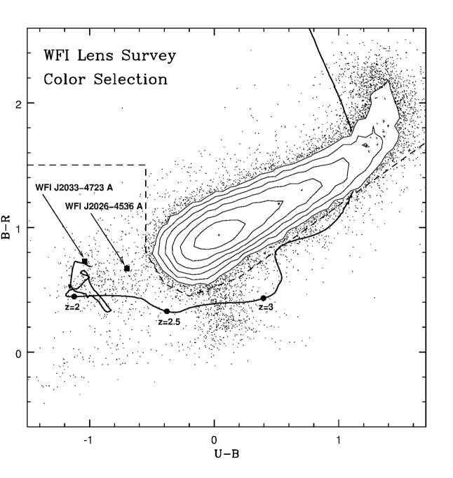
Figure 1: Color-color diagram for $\sim$300 square degrees of WFI survey data. Contours trace the stellar main sequence, and the curved solid line is the quasar color-color track as a function of redshift determined using the FBQS composite quasar spectrum. The dashed line is the color boundary used when selecting gravitationally lensed quasar candidates as described in the text. The positions of the combined A1+A2 components (denoted simply by A) for WFI J2026$-$4536 and WFI J2033$-$4723 are marked by the black squares.

All survey data are processed using a customized pipeline. Source detections and instrumental magnitudes are obtained using a variant of DoPHOT (Schechter, Mateo & Saha 1993), modified to use an empirical point spread function (PSF) for point source photometry. Each WFI image typically contains between 500-1000 objects, which is a sufficient number such that color zeropoints can be obtained from the instrumental colors alone. For example, the $B-R$ colors for each mosaic are calibrated using the “backbone” of the $B$ vs. $B-R$ color-magnitude diagram (e.g., Caldwell & Schechter 1996, their Figure 5), which corresponds to the main sequence turnoff for high Galactic latitude stars. The $U-B$ colors are calibrated by aligning the instrumental main sequence in color-color space to the calibrated stellar main sequence for each mosaic. This yields a well-calibrated color-color diagram for each WFI pointing and allows us to separate quasar candidates from main-sequence stars using a straightforward color cut. This is illustrated in Figure 1, which shows a sample $U-B$ vs. $B-R$ color-color plot of about 300 square degrees (970 mosaic pointings) of survey data. The contours trace the stellar main sequence, and the solid curve is a synthetic quasar track as a function of redshift computed using the FIRST Bright Quasar Survey (FBQS) composite quasar spectrum (Brotherton et al. 2001). Objects that can be decomposed into multiple point sources with at least one component’s colors or the group’s ensemble colors blueward (below) the dashed line in Figure 1 are flagged as gravitational lens candidates.

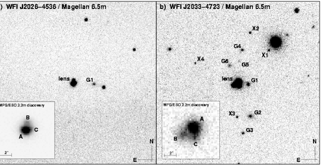
Figure 2: Panel a: Stacked $i$-band observations of WFI J2026$-$4536 taken with the Clay 6.5 m. The lensed quasar and nearby galaxy (G1) are labeled. Panel b: Stacked $i$-band observations of WFI J2033$-$4723 taken with the Clay 6.5 m. Several nearby galaxies (G1-G6) and point-like objects (X1-X4) are labeled. Chart sizes are 1′ square. Insets for both panels show the $R$-band discovery images from the MPG/ESO 2.2 m.

Both WFI J2026$-$4536 (20${}^{\scriptsize{\mbox{h}}}$ 26${}^{\scriptsize\mbox{m}}$ 10$\fs$43, $-45\arcdeg$ 36$\arcmin$ 27$\farcs$1; J2000.0; hereafter J2026) and WFI J2033$-$4723 (20${}^{\scriptsize{\mbox{h}}}$ 33${}^{\scriptsize\mbox{m}}$ 42$\fs$08, $-47\arcdeg$ 23$\arcmin$ 43$\farcs$0; J2000.0; hereafter J2033) were identified as candidate gravitational lenses from the above procedure. The original survey data for J2026 were obtained over a two-week period during April and May 2002, and the data for J2033 were obtained during September 2001. Postage stamps of the $R$-band discovery images for both systems are shown in Figure 2 (insets). DoPHOT resolved both targets into three components in the $B$ and $R$ filters (components A, B and C in Figure 2) and two components (A and B) in the $U$ filter. The AB image separation is 1$\farcs$4 for J2026 and 2$\farcs$5 for J2033. Both systems were also flagged as color-selected quasar candidates (see Figure 1). For J2026, the internally calibrated ($U-B$, $B-R$) colors of components A and B were (-0.7, 0.7) and (-0.6, 0.5), respectively. For J2033, bluer colors of (-1.0, 0.7) and (-0.9, 0.7) were obtained. The multiple image morphology and quasar-like colors provided the initial suspicion that the objects might be gravitationally lensed quasars, and motivated the follow-up observations discussed below.

Figure 2 shows 1′$\times$1′ finder charts centered on both systems. The environment for J2026 (Figure 2a) is relatively clean, with only one other prominent galaxy (G1) in the nearby field. In contrast, the environment for J2033 (Figure 2b) is densely populated, with at least 6 galaxies (G1-G6) within 20″, and several other relatively faint objects (X1-X4) whose profiles are point-like but have yet to be spectroscopically identified.

3 WFI J2026$-$4536 – Follow-up Imaging and Analysis

Follow-up observations of J2026 were obtained on several occasions, with the primary goals of resolving the system’s image morphology, judging the amount of quasar variability, and searching for the foreground lensing galaxy. The quadruple nature of the system was first confirmed during optical re-imaging with the Magellan 6.5 m Clay telescope in April 2003. The lensing galaxy was first detected from IR imaging with the Magellan 6.5 m Baade telescope in September 2003. Second epoch optical data were obtained with the Clay telescope in August, providing a handle on the system variability over a three-month baseline. The system was also imaged with HST in October 2003 yielding precise relative astrometry between the system components and a magnitude estimate of the lensing galaxy. We describe each of these observations below, beginning with the HST data.

3.1 HST/NICMOS – Image Morphology and the Lensing Galaxy

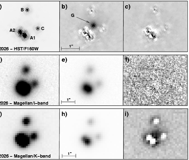
Figure 3: Panel a: Drizzled HST/F160W image of WFI J2026$-$4536. Panel b: Same as (a), but after subtracting the best four-component PSF model. Panel c: Same as (a), but after subtracting the best five-component model including a circularly-symmetric deVaucouleurs profile for the lensing galaxy. The contrast in panels (b) and (c) is the same, stretching from $\pm$1 count second^-1 or equivalently $\pm$2% of A1’s peak. Panel d: Stacked Magellan $i$-band image of WFI J2026$-$4536 taken in 0$\farcs$55 FWHM seeing. Panel e: Same as (d), but at a higher contrast to reveal the A1 and A2 components. Panel f: Same as (d), but after subtracting the best four-component PSF model. Panels g-i: Same as (d)-(f), but for the stacked Magellan $Ks$-band images. All panels have North up and East left.

We observed J2026 with the HST/NICMOS NIC2 camera (plate scale of 0$\farcs$07565 pixel^-1) on 21 October 2003 under the Cycle 12 HST Imaging of Gravitational Lenses program (PI: C. Kochanek; PID 9744). Observations consisted of four dithered MULTIACCUM exposures through the F160W filter ($\approx$ H-band) for a total on-source integration of about 46 minutes. After standard CALNICA processing, bad pixel masks were created for each dithered exposure using the drizzle software of Fruchter & Hook (1997), which were used during the multi-component fitting described below. A drizzled image of the four exposures is shown in Figure 3a and clearly reveals a quadruple image morphology. One can identify the three components detected in the WFI discovery image as the unresolved A1 and A2 components, along with components B and C to the North and West respectively. The system configuration, particularly the bright and closely-separated A1 and A2 images, is a classic inclined-quad lensing configuration (see Saha & Williams 2003), similar to the Northern hemisphere quad PG 1115+080 Weymann et al. (1980), and leaves no doubt that the system is a gravitational lens.

For each dithered image, we have modeled the system’s light distribution using four PSFs generated with the TinyTim v6.1a software of Krist & Hook (2003). The PSFs were generated on a 10$\times$10 oversampled grid to allow for accurate subpixel shifts, taking into account the system’s position on the NICMOS chip and the PAM focus position. Minimization was performed using a Powell (Press et al. 1992) routine. Figure 3b shows the drizzled residuals after subtracting the best-fit models. A fifth component is clearly revealed interior to the four point sources. The object has a peak countrate of $\sim$1% of component A1 and is extended with respect to the NICMOS PSF (gaussian FWHM of 0$\farcs$27 compared to 0$\farcs$13 for point sources). Its position and extent readily identify it as the foreground lensing galaxy (hereafter component G).

We repeated the fit including a circularly-symmetric deVaucoulers profile (convolved with the NICMOS PSF) to account for the lensing galaxy, and solved for the relative positions and intensities of the five components along with the effective radius of the galaxy profile. The averages of the best-fit parameters among the four exposures are listed in Table 1. The separation between the brightest two components is small, only 0$\farcs$33, while the largest separation (A1-B) is 1$\farcs$44. The average effective radius of the galaxy model was 0$\farcs$51 $\pm$ 0$\farcs$18, where the error is from the standard deviation among the four frames.

To compute the galaxy magnitude, we first used an aperture radius of 0$\farcs$38 (5 NICMOS pixels) to sum the galaxy flux in the residual images after the four-component subtraction. The galaxy light in this region is clearly discernible from background and is mostly unaffected by the subtraction residuals, yielding $H=19.56\pm 0.05$. We then computed an aperture correction to large radii ($\sim$11 $R_{\mbox{eff}}$) of 1.13 magnitudes using a synthetic deVaucouleur’s profile (convolved with the PSF) defined by the average $R_{\mbox{eff}}$ of the lensing galaxy. The largest source of systematic error for the final galaxy magnitude given in Table 1 is the effective radius used to compute the aperture correction. Varying $R_{\mbox{eff}}$ by 50% changes the final galaxy magnitude by $\pm$0.4 mags, which is not included in the rms error listed in Table 1. Figure 3c shows the drizzled residuals after subtracting the best-fit five component model, and shows a relatively clean subtraction apart from residuals in the A1 and A2 cores.

3.2 Magellan 6.5 m – Optical Variability

To examine the system’s variability, we obtained first and second epoch observations of J2026 on 24 and 25 April 2003 and 1 and 4 August 2003 at the Las Campanas Magellan Observatories. Data were obtained using the Clay telescope equipped with the Magellan Instant Camera (MagIC), a 2k$\times$2k CCD array with a plate scale of 0$\farcs$06926 pixel^-1. A summary of the observations is given in Table 2.

The April data were bias-subtracted, sky-flattened, and trimmed using standard procedures. Stacked subrasters of the $i$-band exposures are shown at different contrast levels in Figures 3d and 3e. The same image morphology is seen as from the HST data, although the A1 and A2 images are only marginally separated in $i$-band. For the $ugr$-band images, components A1 and A2 appear as a single source because of the poorer seeing.

To obtain the broadband photometric properties of the system, we simultaneously fit four empirical PSFs to each Magellan frame. For the $i$-band data, we allow the position and flux of all four components to vary, but we fix the relative positions for the remaining frames at the averaged $i$-band results. The final relative quasar positions agreed with the NICMOS values to within the rms scatter among the $i$-band frames, and the final $ugri$ quasar magnitudes are listed in Table 1. The proximity of A1 to A2 gives rise to a $\sim 6\%$ scatter in their fluxes, but the sum is tightly constrained with a scatter in $i$ of only 2 millimag. Because of the poorer seeing in the $ugr$ data, only the combined A1 and A2 fluxes are given for these filters. The C/B ratio is constant to within 0.02 mag across $ugri$ and agrees with the NICMOS F160W value, but the (A1+A2)/B ratio shows a significant increase (becoming less equal) of 0.35 mag from $u$ to $i$ and 0.44 mag from $u$ to F160W. Components B and C are also systematically bluer than the combined A1+A2 flux by about 0.2, 0.1 and 0.05 mags across $u-g$, $g-r$, and $r-i$ colors, respectively. This trend is consistent with a color-dependent dimming of either A1 or A2. Unfortunately, the Magellan exposures are not deep enough to provide broadband colors of the lensing galaxy, as seen by the absence of significant structure in the stacked $i$-band residuals (Figure 3f).

For photometric calibration, the Magellan photometry was placed onto the standard Sloan magnitude system using zeropoints derived from the Landolt (1992) standard SA 110-232 and the synthetic Johnson-Kron-Cousins/Sloan magnitude conversions of Fukugita et al. (1996). To help calibrate future observations, Table 1 also lists relative photometry obtained from empirical PSF fitting for eight field stars within 2′ of the lens.

The August $ugri$ data were all taken in non-photometric conditions. The seeing was worse than for the April observations, ranging from 1$\farcs$3 to 1$\farcs$9 in $ugr$ and 0$\farcs$7 to 1$\farcs$0 in $i$, and the four components were resolvable in only two of the $i$-band frames. To measure the total system variability, we have modeled the light profile using fixed relative offsets from the April $i$-band data and calibrated the fluxes using the local standards in Table 1. The total flux from the local standards, measured with respect to each filter’s PSF star, agreed with the April measurements to better than 0.005 mag in $ugi$ and to $0.016$ mag in $r$. We found that the total flux from J2026 has dimmed with respect to the April values by 0.10, 0.08, 0.06, and 0.05 magnitudes in $ugri$, respectively.

3.3 Magellan 6.5 m – IR Field Standards

The lensing galaxy for J2026 was first detected from IR imaging with the Magellan Baade telescope on 14 September 2003 using the Persson’s Auxiliary Nasmyth Infrared Camera (PANIC), which has a 2.2′ square field of view and a plate scale of 0$\farcs$1267 pixel^-1. Dithered 15 second observations were obtained through $H$ and $Ks$ filters with average seeing of 0$\farcs$34 FWHM. The cumulative exposure times were 14 minutes in $H$ and 18 minutes in $Ks$. The stacked $Ks$-band images of J2026 are shown in Figures 3g and 3h, and the corresponding residuals after subtracting a four-component empirical PSF model are shown in Figure 3i. Although the galaxy is visible in the residual panel, the quality of the fit is somewhat poor with significant systematic residuals from each quasar subtraction arising from PSF variations across the chip. The residuals from the over-subtracted cores and under-subtracted wings are stronger than the peak galaxy signal in both the $H$ and $Ks$ images, which makes it difficult to derive an accurate galaxy color. However, the PANIC observations do give a sense for the quality of observations that can be expected from future ground-based IR monitoring of this system. To facilitate detecting future IR variability, we give $H$- and $Ks$-band magnitudes of the four quasar components and nearby field stars intended for use as local standards in Table 1. Magnitudes are again from empirical PSF fitting, with the PSF star placed onto the standard system using Persson et al. (1998) standards #9115 and #9172.

4 WFI J2033$-$4723 – Follow-up Imaging and Analysis

The Magellan follow-up observations for J2033 proceeded along similar lines as for J2026. We obtained follow-up images with the Clay telescope on 1 August 2003 using the same instrumental setup described in §3.2. Single exposures in $ugr$ and several exposures in $i$ were obtained, all in non-photometric conditions. The seeing FWHM ranged between 1$\farcs$0 to 1$\farcs$3 in $ugr$ and between 0$\farcs$5 and 0$\farcs$6 in $i$. A summary of the observations is given in Table 2.

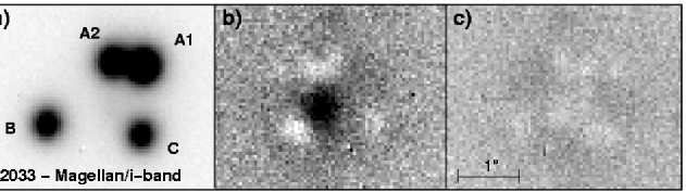
Figure 4: Panel a: Stacked Magellan $i$-band image of WFI J2033$-$4723. Panel b: Same as (a), but after subtracting the best four-component PSF model. Panel c: Same as (a), but after subtracting the best five-component model including a circularly symmetric gaussian profile for the lensing galaxy. The contrast for panels (b) and (c) stretch from -2$\sigma$ to +5$\sigma$, where $\sigma$ is the expected rms per pixel from Poisson and readnoise statistics. All panels have North up and East left.

The data were reduced in the same manner as for J2026. Figure 4a shows the stacked $i$-band image of J2033 and clearly shows four point sources, with component A from the discovery image resolved into components A1 and A2. The image geometry is another inclined-quad, similar to J2026 and again conclusively identifying it as a gravitational lens. To search for the lensing galaxy, we simultaneously fit and subtracted four empirical PSFs to each $i$-band frame. The averaged residuals from the six frames are shown in Figure 4b. A fifth object is now visible in the residual panel, with a peak flux of $\sim$3% that of A1. The object is also extended with a gaussian FWHM of 0$\farcs$81 compared to 0$\farcs$56 for point sources, making its identification as the lensing galaxy certain (hereafter component G). We attempted to model the galaxy with a circularly symmetric deVaucouleurs profile, but the effective radius was poorly constrained. Instead, we use a circularly symmetric gaussian profile and solve for the positions and relative fluxes of the five components for each of the $i$-band frames. The model results are listed in Table 3. To estimate the lensing galaxy magnitude, we used a large (4$\farcs$1) aperture radius on the stacked residuals for the four-component models. No significant residual structure remains after the five-component subtraction, as shown by the stacked residuals in Figure 4c.

Components A1 and A2 were marginally separable by eye in $r$, but appeared as one source in the $u$ and $g$ images because of the poorer seeing. To model the $ugr$ data, we fixed the relative separations at the average $i$-band results and solved for the relative fluxes and the system’s overall position. The galaxy flux in these filters is negligible, so only the four-component model was used. The solutions are again listed in Table 3. As seen for J2026, the flux ratios vary with filter, with the C/B ratio systematically increasing (becoming more equal) by 0.23 mags from $u$ to $i$ and the (A1+A2)/B ratio systematically increasing (becoming less equal) by 0.10 mag from $u$ to $i$. In $r$, where the A1 and A2 fluxes are separable, the (A1+A2)/B change is mostly attributable to a 0.05 mag drop in component A2’s flux from $i$ to $r$.

For future photometric reference, Table 3 also presents photometry from empirical PSF fitting for 7 field stars within 2′ of J2033. The magnitudes have been calibrated using the Landolt (1992) standard Feige 22. Since conditions were nonphotometric during the night, there may be unknown systematic errors in the magnitudes. The $i$-band PSF star had an rms scatter in its aperture magnitude of 0.09 mags over the course of the six consecutive $i$-band exposures, so zeropoint uncertainties of $\sim 0.1$ mag may be present in each filter. Regardless, since magnitudes were determined from relative PSF fitting, the field stars will provide a local set of standards to gauge future variability. The colors from Table 3 are consistent with the known stellar and quasar locus in the Sloan filter system (e.g., Smith et al. 2002, Richards et al. 2001), so zeropoint errors are mostly grey.

5 Spectroscopy

5.1 CTIO 1.5 m Observations

To identify the quasar redshifts, we obtained unresolved spectral observations of both systems on 31 July 2003 using the R-C spectrograph on the CTIO 1.5 m telescope. The low-dispersion grating #13 was used, providing an effective wavelength coverage of 3600 Å to 8000 Å and a dispersion of 5.73 Å pixel^-1. Three 20 minute exposures of each target were taken through a 2″ slit width. Several comparison exposures of He-Ar lamps were also obtained for wavelength calibration. The spectra for each object were reduced using standard IRAF routines and flux calibrated using the spectrophotometric standard Fiege 110.

The unresolved spectra of the two systems are shown in Figures 5a and 5b. Both show typical quasar broad emission lines and underlying continuum. For J2026, a gaussian fit to the peak (top 25% of flux) of the CIV line gives an emission redshift of $z=2.223\pm 0.001$. The CIV feature in quasar spectra is typically blueshifted with respect to the systemic redshift, and indeed we do find a higher redshift estimate of $z=2.237\pm 0.001$ from the Ly$\alpha$, CII and OI/SiIII blended emission lines, but the shift is an order of magnitude larger than that typically found for quasars Vanden Berk et al. (2001). For J2033, we find a systemic redshift of $z=1.661\pm 0.003$ based on a gaussian fit to the peak of the MgII profile.

5.2 Magellan 6.5 m Observations

We also obtained resolved spectral observations of the four quasar images for J2033 on 15 September 2003 using the Inamori Magellan Areal Camera and Spectrograph (IMACS; Bigelow & Dressler 2003) on the Baade telescope. The resolved spectra are valuable for studying effects that depend on position in the lensing galaxy, such as from differential extinction or microlensing. The spectrograph was operated in the long camera mode and read out with 2$\times$2 binning, providing a final pixel scale of 0$\farcs$22 pixel^-1. The 300 lines mm^-1 grating was used, yielding a dispersion of 1.5 Å for each binned pixel and an effective wavelength coverage of 3800 to 8500 Å. We obtained a 300 second exposure of components A1 and A2 and a 600 second exposure of components B and C with the 0$\farcs$75 wide slit held parallel to the respective components in each integration. Exposures of He-Ar lamp lines were also obtained for wavelength calibration.

The spectra were bias-subtracted and flattened using standard procedures. As can be seen in the insets to Figure 6, components B and C are well-resolved along the spatial direction but components A1 and A2 overlap by a fair amount. We used an iterative routine to disentangle the components during the extraction. Each dispersion row was modeled as two overlapping gaussian profiles plus a constant offset for the background sky. For the B and C spectra, the centers, FWHMs, and heights of the gaussians were allowed to vary as a function of wavelength on the initial pass but the two centers and FWHMs were replaced by smoothly varying polynomials as a function of wavelength on subsequent passes. On the final pass, only the heights of the profiles were free to vary. The procedure was similar for the A1 and A2 spectra except that their relative separation was fixed using the Magellan astrometry and the IMACS plate scale derived from the B & C exposure. The best-fit gaussian FWHMs from the extraction ranged from 0$\farcs$5 to 0$\farcs$7, systematically decreasing toward the red. The extracted spectra were then flux calibrated using observations of the spectrophotometric standard LTT7987 Hamuy et al. (1994). The extracted and flux-calibrated spectra for the four components are shown in Figure 6. The gap at 6100 Å is from the physical gap between CCDs in the IMACS camera.

As expected, the individual spectra reveal similarly-redshifted quasars consistent with the CTIO spectrum from §5.1, with appropriately redshifted CIV, CIII], and MgII emission lines for each component. We are primarily interested in the component flux ratios for the broad emission lines and the surrounding continuum for what follows. The line fluxes were determined by fitting a line to the underlying continuum using $\Delta\lambda=200$ Å windows bracketing each emission profile and then summing the continuum-subtracted flux inside a $\Delta\lambda=200$ Å window centered on each profile. Table 4 lists the resulting line fluxes and corresponding wavelength windows. The reported errors bars are based on the uncertainty in the underlying continuum, computed by shifting the continuum up and down by its zeropoint uncertainty. We compare the emission line flux ratios to the broadband values and model predictions in §8 below.

6 Multi-Wavelength Properties

The multi-wavelength properties of the systems were explored by querying the NASA/IPAC Extragalactic Database around each target’s coordinates. No objects were uncovered within 2′ from J2033, but the search did identify a coincident X-ray source from the ROSAT Bright Source Catalog Voges et al. (1999) within 20″ from J2026. The offset is consistent with the 1-2 $\sigma$ positional accuracy of the catalog, so the match is plausible. The quoted ROSAT count rate is 6.8$\pm$2.1 $\times$ 10^-2 cts s^-1 and is several times brighter than other lensed quasars also detected by ROSAT (e.g., PG 1115+080, 1.9$\pm$0.8 10^-2 cts s^-1; RXJ 0911+0551, 2.0$\pm$0.9 10^-2 cts s^-1; Voges et al. 2000).

7 The Lensing Potentials

7.1 WFI J2026$-$4536

The inclined-quad configuration for J2026 implies that the lensed source is located close the diamond caustic but away from the caustic cusps, which produces the two bright and nearly merging components straddling the outer critical curve. If we zero our coordinate system at the lensing galaxy, then the shear axis should point somewhere between the two merging components and the outer critical image. This is roughly East-West for J2026 and toward galaxy G1, the only other prominent galaxy in the field.

We modeled the image positions using the fiducial singular isothermal sphere embedded in an external shear (model ISx). This model has an effective projected potential given by

$$\phi(r,\theta)=br-\frac{\gamma}{2}r^{2}\cos 2(\theta-\theta_{\gamma}),$$ (1)

where $b$ is the potential strength (measured in arcseconds), $\gamma$ is the shear strength, and the adopted sign convection is for $\theta_{\gamma}$ to point toward (or away) from the perturbing mass responsible for the shear. We used the F160W relative positions from Table 1 as constraints and solved for the strengths of the potential and shear, the shear orientation, and the galaxy position using the gravlens software of Keeton (2003). The measured galaxy position was not used as a constraint (denoted by model ISx+). Along with the source position, this gave seven model parameters for the eight position constraints. The best-fit model gave $b=0\farcs 6536$, $\gamma=0.120$ and $\theta_{\gamma}=-90\fdg 5$ East of North. The galaxy center was placed at ($\Delta\alpha$, $\Delta\delta$) = (0$\farcs$0753, -0$\farcs$8168) with respect to image B, which is between 2-3 standard deviations from its measured position. Overall, the model-predicted and observed quasar positions differed by an rms of 0$\farcs$0096. Even though this is formally some five times larger than the scatter in the measured quasar positions, the accuracy is fairly good when compared to other quad lenses with comparable astrometric precision and ISx potential models, which can give rms residuals in the 0$\farcs$02-0$\farcs$04 range. As can be seen in Figure 7a, the source position is indeed close to the inner caustic and gives rise to a net magnification over the unlensed source of about a factor of 30.

The gravitational time delay $\tau$ as a function of the image position $\vec{\theta}$ is given by

$$\tau=\frac{1+z_{l}}{c^{2}}\frac{D_{l}D_{s}}{D_{ls}}\frac{\left[\frac{1}{2}\left(\vec{\theta}-\vec{\beta}\right)^{2}-\phi\right]}{206265},$$ (2)

where $\vec{\beta}$ is the source position and $D_{l},D_{s}$, and $D_{ls}$ are angular diameter distances between the observer and lens, observer and source, and lens and source, respectively. Since the lens redshift for J2026 is unknown, we give time delay estimates using the quantity in square brackets which can be computed using the observed image positions and ISx model parameters alone. In Table 5 we give the predicted image positions for the four images and lensing galaxy, the image magnifications and the time delays. A negative magnification denotes a parity flip in the lensed image, arising from a saddlepoint in the time delay surface. Images A2 and C are saddlepoints, which can also be seen from the time delay contours in Figure 7b. The leading image for the lens is B, followed by A1, A2, and C.

Lacking a spectroscopic redshift for the lensing galaxy, we can estimate its redshift using the potential model and the IR magnitude of the lensing galaxy from §3.1. The potential strength $b$ is related to the halo velocity dispersion $\sigma$ by

$$b=\frac{D_{ls}}{D_{s}}\frac{4\pi\sigma^{2}}{c^{2}}$$ (3)

(Narayan & Bartlemann 1999). Knowing $\sigma$, the galaxy’s $B$-band luminosity can be estimated from the Faber-Jackson (1976) relationship $L/L_{\star}=\left(\sigma/\sigma_{\star}\right)^{\gamma}$, where $L_{\star}$ corresponds to a $B$-band absolute magnitude of $M_{B,\star}=-19.7+5\log h$ (assuming $H_{\rm{o}}=100h$ km s^-1 Mpc^-1) and we adopt $\gamma=4.0$ and $\sigma_{\star}=220$ km s^-1 appropriate for elliptical galaxies. Given $M_{B}$, the galaxy’s observed F160W magnitude then follows from

$$m_{F160W}=M_{B}+DM(z_{l})+K_{B,F160W}(z_{l}),$$ (4)

where $DM$ is the cosmological distance modulus and $K_{B,F160W}$ is the generalized K-correction from the galaxy’s rest-frame $B$-band magnitude to the observed-frame F160W magnitude (e.g., Hogg et al. 2002). The K-corrections are computed using the Bruzual & Charlot (2003) spectral evolution code. We use a solar-metallicity, passively-evolving instantaneous burst model where all stars form at $z_{f}=3.0$, which is consistent with the observed colors of most other lensing galaxies (Kochanek et al. 2000). Figure 8a shows the predicted $m_{F160W}$ magnitudes as a function of the lens redshift (curved solid line) and the observed F160W galaxy magnitude from §3.1 (horizontal line). In principle, the matching redshifts are around $z_{l}\sim 0.4$ and $z_{l}\sim 1.9$, although the higher redshift is ruled out since a velocity dispersion of 520 km s^-1 would be required to produce the observed image separations. At $z_{l}=0.4$, the required lens velocity dispersion is reasonable, 180 km s^-1 (0.4 $L_{\star}$), and the ISx model predicts a long time delay (B-C) of 7.5 days and a short delay (A1-A2) of 2.4 hours. Placing the lens at $z_{l}=0.3$ or $z_{l}=0.6$ yields B-C delays of 5.3 or 12.8 days, respectively.

The shear PA points within 8° of galaxy G1 and identifies it as the likely source of the perturbation. At a distance of 7$\farcs$4 from the position of the lensing galaxy, the shear strength implies a potential strength for G1 of $b=1\farcs 78$, or 2.7 times larger than for the primary lens. This compares well with the relative fluxes of the two galaxies. The galaxy’s potential strength $b$ should scale with the square root of its luminosity for a $\gamma=4$ Faber-Jackson exponent, so we expect a G/G1 flux ratio of 7.4 based on the ISx+ model. The observed F160W flux ratio inside a 0$\farcs$38 aperture radius is 6.0, roughly consistent with the prediction.

7.2 WFI J2033$-$4723

The image configuration for J2033 is qualitatively similar to J2026, so we started with the ISx model with the lens galaxy first fixed at the observed $i$-band position. This gave five parameters for the eight position constraints. The best-fit model yielded an rms between predicted and observed positions of 0$\farcs$085, almost an order of magnitude worse compared to the ISx+ model for J2026. Allowing the center of the potential to float (model ISx+) improved the situation somewhat, with a final rms of 0$\farcs$056, but is still poor with respect to the J2026 model results.

One way to improve the model is to allow more angular freedom in the potential. Figure 2b shows that two shear axes may be needed: the galaxy G1 due West of the lens and the G4-G5-G6 and G2-G3-X3 groups to the North and South. We again adopted a ISx model for the main lensing galaxy but also placed a SIS potential at the position of G1 (model ISISx). The position of both the lensing galaxy and G1 were fixed at their measured positions in Table 3, giving six parameters for the eight position constraints. This gave a final rms between observed and predicted positions of 0$\farcs$029 and is roughly a factor of two improvement over the ISx+ model with only one additional free parameter. The potential strength of G1 is larger than for the main lensing galaxy, $b=1\farcs 24$ compared to $b=0\farcs 94$, and the shear strength is $\gamma=0.253$ and points at a PA of 10$\fdg$5 East of North. This roughly coincides with the location of the G4-G5-G6 and G2-G3-X3 groups.

One final improvement is to allow the center of the lensing galaxy’s potential to float (ISISx+). This leaves no degrees of freedom and we expect a perfect fit to the observations. The best-fit model reproduced the observed image positions precisely, but the final lensing galaxy position shifted only 0$\farcs$041 from the average $i$-band position. This is well within our measurement errors for component G. The potential strength of the lensing galaxy was $b=0\farcs 98$ and the shear direction was $\theta_{\gamma}$ = 12$\fdg$5 East of North. This is mostly unchanged from the ISISx model, but the strengths of G1 and the shear dropped to $b=0\farcs 95$ and $\gamma=0.225$, suggesting that this may be a more realistic model.

In Table 6 we give the observed and predicted positions for the four images from the ISISx+ model, as well as the image magnifications and predicted time delays. Figure 7c shows the source position near the inner edge of the diamond caustic and that the inner caustic is shifted by some 2″ westward of the lensing galaxy center because of the G1 perturbation. The net amplification of the background quasar is about a factor of 20 over its unlensed flux.

One can see from the time delay contours in Figure 7d that images A2 and C are saddlepoints and images A1 and B are minima. The time delay order is the same as for J2026, namely B, A1, A2, and C. Figure 8b shows the estimated $i$-band magnitude of the lensing galaxy as a function of redshift as constrained by the system’s image separation and source redshift, using the same method described in §7.1. The predicted magnitudes suggest a lens redshift in the vicinity of $z_{l}\sim 0.4$ or $z_{l}\sim 1.5$, but the higher redshift is again ruled out by the implied velocity dispersion (990 km s^-1). The required velocity dispersion at $z_{l}=0.4$ is 220 km s^-1, or roughly an $L_{\star}$ galaxy. Assuming a lens redshift of $z_{l}=0.4$, the largest differential time delay (B-C) is 26.0 days and the shortest (A1-A2) is 1.0 days, although the long delay ranges from 18.0 to 47.0 days for respective lens redshifts of $z_{l}=0.3$ or $z_{l}=0.6$.

8 Anomalous Flux Ratios and Evidence for Microlensing

Several of the observed flux ratios for J2026 and J2033 vary with wavelength and differ significantly from the model predictions. For example, the (A1+A2)/B flux ratios for both systems drop by 0.1-0.3 mags from $i$ to $u$, while the C/B $i$-band ratios differ by 0.2-0.3 mags from the model values. Both trends are much larger than the photometric accuracy. Such anomalous flux ratios are found in other lensed quasars as well, and several theories have emerged to explain the differences. Metcalf & Zhao (2002) argue that unmodeled substructure near the lensing galaxy can significantly perturb the magnifications of the lensed images while leaving the image positions mostly unchanged. This produces a constant achromatic effect and essentially implies that the problem stems from the use of oversimplistic macromodels. Schechter & Wambsganss (2002) argue that microlensing by stars in the lensing galaxy can significantly perturb the observed flux ratios, particularly by demagnifying the flux from saddlepoint images, leading to a time-varying chromatic effect. Of course, more mundane explanations like dust extinction are also possible (e.g., Falco et al. 1999) when working with optical fluxes, leading to a constant chromatic effect that can be difficult to disentangle from microlensing-induced variations.

While a combination of these factors might be at work for any given system, microlensing is perhaps the easiest to identify because of the time and color dependence. In particular, the microlensing-induced variations ought to depend on the intrinsic source size: larger sources will cover more of the caustic network, which will wash out the microlensing signal and leave flux ratios that approach the macromodel values. For quasar accretion disks, this leads to stronger and more frequent continuum variations in the blue. At the other extreme, the quasar’s broad line region, which is at least an order of magnitude larger than the continuum-emitting disk (Kaspi et al. 2000, Kochanek 2003), ought to be much less affected by microlensing. An example of the latter can be found in the quadruple quasar HE 0435-1223 (Wisotzki et al. 2003), which shows emission line ratios that agree better with the model predictions than do the broadband flux ratios, although the match is still not perfect.

For J2026, we find evidence for microlensing from the system’s broadband flux ratios and time variability. The combined (A1+A2)/B flux ratio shows a strong wavelength dependence, systematically increasing from 4.29 in $u$ to 5.90 in $i$, a difference of 0.35 mags. The trend is likely due to varying A1+A2 flux rather than from component B, since the C/B ratio is constant to within 0.02 mag from $u$ to $i$ and thus each component is probably not significantly affected by microlensing or dust. This implies that there is less A1+A2 flux at bluer wavelengths than expected from the overall shape of the B and C quasar spectra. The likely causes are either dust extinction or microlensing demagnification of one of the A components. Patchy dust has an even chance of obscuring either A1 or A2, but a significant microlensing demagnification should preferentially occur in the saddlepoint image A2 according to Schechter & Wambsganss (2002). Although the poor seeing prevents us from determining which component is responsible for the trend, the second epoch observations do suggest that microlensing is present. The three-month variability is larger in the blue ($\Delta m=0.10$ mag) than in the red ($\Delta m=0.05$ mag), consistent enhanced microlensing fluctuations expected from smaller source sizes.

It is also interesting that the C/B flux ratio, although mostly constant from $u$ to $Ks$ and thus probably not significantly affected by microlensing or dust, still differs by 0.2 mags from the model prediction. In this case, the discrepancy may reflect a shortcoming in the model which used only the image positions as constraints. To check this, we repeated the ISx+ model using the observed $i$-band C/B ratio as a constraint, but we had to tighten the B and C flux uncertainties to 0.1% before the model successfully reproduced the obseved ratio. The final rms between the observed and predicted quasar positions was 0$\farcs$015, still typical of other quadruple lenses, but the required shear increased by 25% and the final galaxy position shifted by 0$\farcs$032, or about 4$\sigma$ from its measured position. So the model can be forced to fit C/B ratio, although the stronger shear and misaligned center suggests it is less realistic. More complicated models, perhaps taking into account asymmetries or substructure in the galaxy potential, are probably required to give a satisfying result.

For J2033, we find evidence for microlensing mostly from the C/B flux ratio. The ratio increases from 0.75 in $u$ to 0.93 in $i$, a difference of 0.23 mags, again suggesting either dust extinction or microlensing. However, even the $i$-band ratio differs by 0.3 mags from the model prediction of 1.22. Yet the agreement is strikingly improved when the model is compared to the IMACS emission line flux ratios. Figure 9a shows the $m_{C}-m_{B}$ magnitude differences obtained from the emission line fluxes and bracketing continuum. Each emission feature has three measurements: the line ratio from Table 4 and the flanking continuum ratios from the IMACS spectra. The continuum ratios systematically tend toward the model prediction (horizontal line) as one moves from blue to red, as do the broadband flux ratios (open circles). However, the emission line ratios are systematically larger than the bracketing continuum for each emission feature, and are mostly in agreement with the macromodel predictions. The effect is most noticeable for CIV and CIII], yielding C/B ratios clearly greater than unity, a feature not found in either the continuum or broadband ratios. The different emission line and continuum ratios rule out significant dust extinction, which ought to affect both measurements equally, leaving microlensing as the likely explanation for the flux ratio trend. There is also evidence for 0.2 mag variability in the C/B flux ratio between the Magellan broadband measurements and the continuum ratios, suggesting some combination of microlensing and intrinsic quasar variability over the 1 month baseline.

A smaller color trend is found for the (A1+A2)/B broadband ratios, which increase from 2.72 in $u$ to 2.99 in $i$, a 0.10 mag difference. Figure 9b shows the A2/A1 IMACS ratios similar to the C/B plot described above, but the noise from the extraction masks any trend that might be present in the emission line or continuum ratios. At best, one can say that the line ratios are consistent with the model predictions and broadband flux ratios.

9 Summary and Conclusions

We have reported the discovery of two bright gravitationally lensed quasars found during a wide-field optical survey for lenses in the Southern hemisphere. WFI J2026$-$4536 ($g=16.5$, source redshift of $z_{s}=2.23$) and WFI J2033$-$4723 ($g\approx 17.9$, $z_{s}=1.66$) are both quadruple systems that share similar inclined-quad image configurations with maximum image separations of 1$\farcs$4 and 2$\farcs$5, respectively. The lensing galaxies are detected for both systems.

For J2026, the small image separation leads to relatively short differential time delays ranging from 1-2 weeks for the long delay (B-C) to several hours for the short delay (A1-A2), depending on the lensing galaxy’s redshift. Even the long delay will be difficult to measure from optical monitoring campaigns unless the quasar is uncharacteristically variable on such timescales. This may limit the usefulness of J2026 for cosmological applications but makes it an attractive target for microlensing studies since intrinsic variability will not be easily confused with microlensing-induced signals. The (A1+A2)/B flux ratio varies by 0.37 mags from $u$ to $Ks$, strongly suggesting either microlensing or dust extinction, while the enhanced variability observed in the blue over three months suggests at least some microlensing-induced variability. Ground-based monitoring will help to gauge the presence of microlensing, but will be a challenge for the A1 and A2 components given the small image separation.

The ROSAT detection of J2026 also opens the prospect of measuring an X-ray time delay between the short-delay components. The A1-A2 delay is on the order of hours and could be measured during a single Chandra observations if significant X-ray variability is present. Since Chandra would be unable to spatially separate the A1 and A2 components, the approach would require autocorrelating their unresolved lightcurve as originally suggested by Chartas et al. (2001).

For J2033, the larger image separations yield longer differential time delays and will also make ground-based monitoring an easier task. The longest time delay (B-C) is predicted to be 1-2 months, again depending on the lens redshift. However, the lensing potential is more complicated than for J2026, with a group of at least six galaxies within 20″ that require two separate perturbation axes for effective modeling. The complex potential may complicate the interpretation of any measured delay. This system is also an attractive target for microlensing studies. The system’s C/B flux ratio varies by 0.23 mags from $u$ to $i$, while the C/B emission line ratios agree much better with the macromodel predictions than either the continuum or broadband values, as expected from microlensing magnifications that ought to depend on the source size. The emission line ratios suggest that the anomalous C/B flux ratio in the blue is caused primarily by microlensing-induced perturbations rather than unmodeled substructure in the lensing potential, as might be expected given the ratio’s strong color trend.

The redshifts of both lensing galaxies are still needed to yield a precise time delay prediction, and spectroscopic identification of nearby field objects, particularly the nearby G1 galaxies and the galaxy group surrounding J2033, will help to construct more accurate lensing models. In view of the two systems’ optical brightness, demonstrated variability, and evidence for microlensing, it is clear that future monitoring will be a worthwhile undertaking.

Table 1: Relative Astrometry and Photometry for WFI J2026$-$4536 and Field

ID	$\Delta\alpha$ (″)	$\Delta\delta$ (″)	$u$	$g$	$r$	$i$	$H$	$F160W$	$Ks$
A1	+0.1621(0014)	-1.4281(0009)	—	—	—	17.109(059)	15.585	15.252(013)	14.978
A2	+0.4149(0014)	-1.2133(0009)	—	—	—	17.363(073)	16.107	15.673(008)	15.371
A1+A2	—	—	17.336	16.816	16.557	16.475(003)	15.062	14.690(008)	14.404
B	$\equiv 0$	$\equiv 0$	18.916	18.581	18.450	18.402(012)	17.054	16.709(009)	16.359
C	-0.5722(0015)	-1.0436(0004)	19.145	18.814	18.666	18.625(011)	17.208	16.916(010)	16.559
G	-0.0813(0031)	-0.7967(0068)	—	—	—	—	—	18.43(05)	—
G1	-7.398(026)	-1.940(006)	22.948	21.931	20.863	20.160(011)	17.493	—	16.848
7	16.5	41.9	23.500	20.774	19.519	18.597(050)	—	—	—
10	-50.8	40.8	18.336	16.947	16.463	16.311(001)	15.080	—	15.094
12	49.9	36.3	17.145	15.462	14.850	14.644(035)	—	—	—
15	-6.0	21.9	21.088	19.510	18.921	18.656(059)	17.122	—	17.161
18	-23.1	9.8	20.517	19.628	19.332	19.215(123)	18.116	—	18.266
19	31.0	1.8	21.084	20.145	19.753	19.562(031)	—	—	—
25	41.0	-36.6	21.885	19.479	18.528	18.134(028)	—	—	—
28	24.7	-55.0	21.918	19.761	18.961	18.630(075)	—	—	—

Note. — Relative photometry and astrometry results for WFI J2026$-$4536 and field. Error bars, when present, are from the rms scatter among frames. The $ugri$ data are from the April Magellan run. The G1 position is measured from the Magellan $i$-band frames. Relative positions for the quasar components and the lensing galaxy are from the HST/F160W frames. Galaxy G1 $ugri$ photometry was computed using a circular aperture with radius of 0$\farcs$7, while the F160W magnitude for component G was computed as described in the text. For the Magellan data, the psf star was #10 for the the $r,i,H,Ks$ filters, and #12 for the $u$,$g$ filters.

Table 2: Summary of Magellan Optical Observations

Target	filter	Date (UT)	$N_{im}$	$<$Exp$>$ (s)	$<$FWHM$>$ (″)
WFI J2026$-$4536	$u$	24 Apr 03	1	360	1.07
	$g$	24 Apr 03	1	120	0.98
	$r$	24 Apr 03	1	120	0.90
	$i$	25 Apr 03	3	120	0.55
	$u$	1 Aug 03	1	240	1.87
	$g$	4 Aug 03	1	120	1.52
	$r$	4 Aug 03	1	120	1.34
	$i$	4 Aug 03	5	120	0.86
WFI J2033$-$4723	$u$	1 Aug 03	1	240	0.96
	$g$	1 Aug 03	1	120	1.31
	$r$	1 Aug 03	1	120	0.94
	$i$	1 Aug 03	6	120	0.56

Table 3: Relative Astrometry and Photometry for WFI J2033$-$4723 and Field

ID	$\Delta\alpha$ (″)	$\Delta\delta$ (″)	$u$	$g$	$r$	$i$
A1	-2.193(03)	1.258(02)	—	—	18.839	18.682(005)
A2	-1.477(03)	1.368(02)	—	—	19.346	19.144(005)
A1+A2	—	—	18.749	18.473	18.311	18.136(004)
B	$\equiv$0	$\equiv 0$	19.836	19.606	19.478	19.327(006)
C	-2.108(03)	-0.282(03)	20.151	19.760	19.600	19.409(012)
G	-1.412(33)	0.277(20)	—	—	—	19.713
G1	-5.397(10)	0.247(10)	—	—	—	—
32	-5.7	69.7	20.715	19.659	19.221	19.130(006)
33	57.9	69.2	20.386	18.256	17.482	17.214(001)
36	-32.5	62.1	20.495	19.588	19.195	19.127(005)
38	-0.9	61.6	19.625	17.169	16.211	15.844(004)
55	-15.7	15.6	17.726	16.613	16.220	16.149(003)
61	60.4	-2.4	—	19.252	18.210	17.884(000)
76	-40.8	-43.5	—	21.425	20.163	18.871(003)

Note. — Relative photometry and astrometry results for WFI J2033$-$4723 and field. Error bars, when present, are from the rms scatter among frames. The psf stars were #55, 38, and 61 for the $u$, $g$, and $r,i$ filters, respectively. Galaxy photometry for component G was computed as described in the text. Note that the data were obtained under nonphotometric conditions, with possible zeropoint errors of $\sim 0.1$ mag in each filter.

Table 4: Emission Line Fluxes for WFI J2033$-$4723

Feature	$\Delta\lambda$ (Å)	A1	A2	B	C
CIV	[4000,4200]	63.3(23.6)	47.2(21.0)	49.1(11.5)	72.5(13.0)
CIII]	[4950,5150]	43.8(8.1)	33.0(7.0)	27.6(3.7)	39.7(3.9)
MgII	[7350,7550]	36.2(7.9)	22.5(6.2)	23.0(3.7)	29.1(3.4)

Note. — $\Delta\lambda$ defines the wavelength window used to measure each emission line flux. Fluxes are in units of 10^-16 ergs s^-1 cm^-2.

Table 5: ISx+ Model Results for WFI J2026$-$4536

ID	$\Delta\alpha$ (″)	$\Delta\delta$ (″)	$\mu$	$t$
A1	0.1653	-1.4295	12.27	-0.1944
A2	0.4069	-1.2033	-10.27	-0.1927
B	0.0091	0.0010	3.53	-0.2956
C	-0.5764	-1.0533	-3.50	-0.1627
G	0.0753	-0.8168	—	—

Note. — Listed are the predicted image and galaxy positions, the model magnifications ($\mu$), and dimensionless time delays ($t$) as described in the text. The coordinate system is centered on the observed position of image B.

Table 6: ISISx+ Model Results for WFI J2033$-$4723

ID	$\Delta\alpha$ (″)	$\Delta\delta$ (″)	$\mu$	$t$
A1	-2.192	1.257	7.70	-3.997
A2	-1.476	1.366	-5.90	-3.981
B	0.000	0.000	3.42	-4.274
C	-2.103	-0.278	-4.18	-3.846
G	-1.419	0.326	—	—

Note. — Listed are the predicted image and galaxy positions, the model magnifications ($\mu$), and dimensionless time delays ($t$) as described in the text. The coordinate system is centered on the observed position of image B.

Figure 5: Unresolved long-slit spectra of WFI J2026$-$4536 (panel a) and WFI J2033$-$4723 (panel b) obtained with the CTIO 1.5 m. Prominent emission lines are labeled for both quasars.

Figure 6: Resolved spectra of the four WFI J2033$-$4723 quasar components obtained with the Magellan/IMACS spectrograph. For clarity, the A1, B, and C spectra have been shifted by 0.3, -0.6, and -1.1 dex, respectively. Bin sizes are 13.5 Å (9 pixels) for the A1 and A2 spectra and 7.5 Å (5 pixels) for the B and C spectra. Insets show a slice along the dispersion direction (as a function of pixel number) in the vicinity of the MgII emission profile for A1 and A2 (left histogram) and for B and C (right histogram), along with the double gaussian solutions for the respective slices (A1 and C: solid lines; A2 and B: dashed lines).

Figure 7: Panel a: ISx+ model results for WFI J2026$-$4536 showing the inner diamond caustic and outer critical line, the predicted image positions (squares), the observed image positions (triangles), and the model source position (open circle). Panel b: Contour plot of WFI J2026$-$4536 time delay function. Panels c and d: Same as (a) and (b), but showing ISISx+ model results for WFI J2033$-$4723.

Figure 8: Predicted lensing galaxy magnitudes for WFI J2026$-$4536 (panel a) and WFI J2033$-$4723 (panel b) as a function of the lens redshift (solid curve), along with $\pm 1\sigma$ errors (dashed curves) expected from the scatter in the Faber-Jackson relationship (Dressler et al. 1987). The horizontal lines are the measured galaxy magnitudes.

Figure 9: Panel a: Magnitude differences for WFI J2033$-$4723 components B and C as a function of observed wavelength. Solid points are from IMACS spectra and are grouped in three’s for each emission feature, consisting of the central emission line ratio and the two bracketing continuum ratios. Open circles are the Magellan broadband $ugri$ flux ratios obtained one month earlier. Panel b: Same as (a), but for WFI J2033$-$4723 components A1 and A2.

References

- Bigelow & Dressler (2003) Bigelow, B. C. & Dressler, A. M. 2003, Proc. SPIE, 4841, 1727
- Boyle et al. (1988) Boyle, B. J., Shanks, T. & Peterson, B. A. 1988, MNRAS, 235, 935
- Brotherton et al. (2001) Brotherton, M. S., Tran, H. D., Becker, R. H., Gregg, M. D., Laurent-Muehleisen, S. A. & White, R. L. 2001, ApJ, 546, 775
- Bruzual & Charlot (2003) Bruzual, G. & Charlot, S. 2003, MNRAS, 344, 1000
- Caldwell & Schechter (1996) Caldwell, J. A. R. & Schechter, P. L. 1996, AJ, 112, 772
- Chartas et al. (2001) Chartas, G., Dai, X., Gallagher, S. C., Garmire, G. P., Bautz, M. W., Schechter, P. L., Morgan, N. D. 2001, ApJ, 558, 119
- Claeskens et al. (1996) Claeskens, J.-F., Surdej, J. & Remy, M. 1996, A&A, 305, 9
- Dalal & Kochanek (2002) Dalal, N. & Kochanek, C. S. 2002, ApJ, 572, 25
- Dressler et al. (1987) Dressler, A., Lynden-Bell, D., Burstein, D., Davies, R. L., Faber, S. M., Terlevich, R. & Wegner, G. 1987, ApJ, 313, 42
- Faber & Jackson (1976) Faber, S. M. & Jackson, R. E. 1976 ApJ, 204, 668
- Falco et al. (1999) Falco, E. E., Impey, C. D., Kochanek, C. S., Lehár, J., McLeod, B. A., Rix, H.-W., Keeton, C. R., Muñoz, J. A. & Peng, C. Y. 1999, ApJ, 523, 617
- Fruchter & Hook (1997) Fruchter, A. & Hook, R. N. 1997, Proc. SPIE, 3164, 120
- Fukugita et al. (1996) Fukugita, M., Ichikawa, T., Gunn, J. E., Doi, M., Shimasaku, K. & Schneider, D. P. 1996, AJ, 111, 1748
- Gregg et al. (2001) Gregg, M. D., Becker, R. H., Schechter, P. L., White, R. L. & Wisotzki, L. 2000, AJ, 119, 2535
- Hamuy et al. (1994) Hamuy, M., Suntzeff, N. B., Heathcote, S. R., Walker, A. R., Gigoux, P. & Phillips, M. M. 1994, PASP, 106, 566
- Hogg et al. (2002) Hogg, D. W., Baldry, I. K., Blanton, M. R. & Eisenstein, D. J. 2002, astro-ph/0210394
- Kaspi et al. (2000) Kaspi, S., Smith, P. S., Netzer, H., Maoz, D., Jannuzi, B. T. & Giveon, U. 2000, ApJ, 533, 631
- Keeton (2003) Keeton, C. 2003, astro-ph/0102340
- Kochanek (1991) Kochanek, C. S. 1991, ApJ, 379, 517
- Kochanek et al. (2000) Kochanek, C. S., Falco, E. E., Impey, C. D., Lehár, J., McLeod, B. A., Rix, H.-W., Keeton, C. R., Muñoz, J. A. Peng & C. Y. 2000, ApJ, 543, 131
- Kochanek et al. (2002) Kochanek, C. S. 2002, ApJ, 578, 25
- Kochanek (2003) Kochanek, C. S. 2003, submitted to ApJ, astro-ph/0307422
- Koopmans et al. (2001) Koopmans, L. V. E. & the CLASS collaboration 2001, Publ. Astron. Soc. Australia, 18, 179
- Krist & Hook (2003) Krist, J. E. & Hook, R. N. 2003, The Tiny Tim User’s Guide, version 6.1a (Baltimore: STScI)
- Landolt (1992) Landolt, A. U. 1992, AJ, 104, 340
- Maza et al. (1996) Maza, J., Wischnjewsky, M. & Antezana, R. 1996, RMxAA, 32, 35
- Metcalf & Zhao (2002) Metcalf, R. B. & Zhao, H. 2002, ApJ, 567, L5
- Morgan et al. (1999) Morgan, N. D., Dressler, A., Maza, J., Schechter, P. L. & Winn, J. N. 1999, 118, 1444
- Morgan et al. (2003) Morgan, N. D., Gregg, M. D., Wisotzki, L., Becker, R., Maza, J., Schechter, P. L. & White, R. L. 2003, AJ, 126, 696