Supernova Properties from Shock Breakout X-rays

Abstract

We investigate the potential of the upcoming LOBSTER space observatory (due circa 2009) to detect soft X-ray flashes from shock breakout in supernovae, primarily from Type II events. LOBSTER should discover many SN breakout flashes, although the number is sensitive to the uncertain distribution of extragalactic gas columns. X-ray data will constrain the radii of their progenitor stars far more tightly than can be accomplished with optical observations of the SN light curve. We anticipate the appearance of blue supergiant explosions (SN 1987A analogs), which will uncover a population of these underluminous events. We consider also how the mass, explosion energy, and absorbing column can be constrained from X-ray observables alone and with the assistance of optically-determined distances. These conclusions are drawn using known scaling relations to extrapolate, from previous numerical calculations, the LOBSTER response to explosions with a broad range of parameters. We comment on a small population of flashes with $0.2<z<0.8$ that should exist as transient background events in XMM, Chandra, and ROSAT integrations.

1 Introduction and Motivation

A core collapse supernova produces no electromagnetic radiation until its envelope is completely consumed by the explosion fireball. This phase ends, however, with a brilliant flash of X-ray or extreme ultraviolet photons heralding the arrival of the fireball shock at the stellar surface. The “breakout” flash is delayed in time, and vastly reduced in energy, relative to the neutrino and gravity-wave transients produced by core collapse. However, it conveys useful information about the explosion and the star that gave rise to it.

We are motivated to explore the detection and interpretation of such flashes by several points. First, breakout flashes provide strong constraints on some properties of their presupernova stars that are poorly determined from the optical light curve. Second, whereas previous searches for these flashes have failed, the planned LOBSTER experiment should routinely discover them. Third, this experiment will report (within minutes) the location of almost any core-collapse supernova (some flashes are extincted) within its field of view to a distance of many megaparsecs. Data will be downlinked to Earth every 90 minutes and analysed via an automated process. This allows rapid optical follow-up and, in the unlikely case of a very nearby explosion, correlation with neutrino and gravity-wave signals. Early warning and the precise timing of explosion are valuable for the interpretation of the optical light curve: for instance, in calibration of the Expanding Photospheres Method for distance determination. Fourth, flash-selected surveys of Type II supernovae are less biased by competition with light from galactic nuclei than are optical surveys. Finally, there exists the possibility that LOBSTER or a subsequent instrument could detect the signature of asymmetry in the supernova explosion through its effects on the breakout flash.

In this paper we consider primarily what can be determined about the stellar progenitor from the X-ray flash alone, from the flash and an optical distance, or from the delay separating the flash from the core collapse. Our investigation is based on previous numerical calculations of the breakout flash spectrum, primarily by Klein & Chevalier (1978), Ensman & Burrows (1992), Blinnikov et al. (1998), and Blinnikov et al. (2000), and on the analytical approximations and scalings derived by Matzner & McKee (1999). Our consideration of observational points relies on technical details kindly provided by Nigel Bannister and the LOBSTER science team.

1.1 Limitations of Optical Light Curves for Constraining SN Properties

Supernova properties provide a datum at the end of stellar evolution. Collectively, such data from many stars reveal how the intrinsic properties (e.g., initial mass, rotation, metallicity) and extrinsic properties (e.g., binary membership and separation) of massive stars affect their evolution. It is currently uncertain, for instance, how many supernovae come from relatively compact blue supergiant progenitors and therefore produce underluminous light curves like that of SN 1987A (Schmitz & Gaskel, 1988; Fillipenko, 1988; Young & Branch, 1988; van den Bergh & McClure, 1989; Schaefer, 1996). This arises both from a bias against detecting small progenitors, and a bias to overestimate the radius, as discussed below. X-ray observations have the potential to mitigate the former bias (Table 4) and eliminate the latter (§3).

Using the scaling relations of Litvinova & Nadëzhin (1985), Hamuy (2003) estimated progenitor properties from the plateau properties of the 13 best-measured Type IIP SNe (the only ones for which sufficient observations exist; prior to his work, only SN 1969C had been analyzed in this fashion). Based on measurement error, he assigned $1\sigma$ uncertainties of roughly 0.26 dex (a factor of 1.8) to the derived radii (and similar uncertainties to mass and explosion energy). Several additional sources of uncertainty degrade the determination of progenitor radius derived from optical data.

For one, there is an uncertainty in the underlying distribution of ejecta density and opacity. The scaling relations of Litvinova & Nadëzhin (1985) are derived from a suite of numerical simulations involving an explosion in a simplified version of a red supergiant (RSG) model, in which the progenitor density scales with radius as $\rho_{0}\propto(1-r/R_{\star})^{1/8}$, where $R_{\star}$ is the size of the star. Popov (1993), in comparison, developed analytical formulae for plateau-type light curves, assuming a constant density distribution in the ejecta. Although Litvinova & Nadëzhin’s results are nominally more precise, being derived from a hydrodynamical calculation of a model star, neither set of formulae account in detail for the presupernova structure of the progenitor – which depends, for instance, on the mass ratio between the star’s mantle and its hydrogen envelope. (Simple formulae for the ejecta distributions from supergiants have been presented by Matzner & McKee (1999), but have not yet been used to predict light curves). For a typical plateau light curve (absolute V magnitude peaking at -17.5^mag at 70 days; early photospheric velocity 7000 km/s; Popov, 1993), the Litvinova & Nadëzhin and Popov determinations of $R_{\star}$ differ by 0.28 dex or a factor of 1.9, which is comparable to the observational uncertainties. This serves as an estimate (although probably an overestimate) for the errors due to an unknown ejecta distribution.

Additionally, there is a bias toward large values of $R_{\star}$ due to the contamination of the plateau peak by the radioactive decay of ⁵⁶Co produced in the explosion. The formulae of Litvinova & Nadëzhin (1985) and Popov (1993) assume the light curve to be powered by heat deposited in the ejecta by the explosion shock itself. At the time that photons can diffuse out of the ejecta, this heat supply has been adiabatically degraded during expansion; the fraction remaining is inversely proportional to the initial stellar radius. In contrast, ⁵⁶Co, with a half-life of 77.3 days, releases its energy during the plateau. If the initial radius is small enough, cobalt decay will compete with or even dominate shock-deposited heat. To detect this effect, one must monitor the late-time decay of the light curve to estimate the cobalt contribution. Nevertheless, the derived progenitor radii are easily corrupted, because there is no simple way to subtract the radioactive contribution from the light curve; nor is this possible, if the ⁵⁶Co luminosity exceeds that from shock heating. Using the Popov (1993) formulae, we find that radioactivity dominates when

$$\frac{M_{{}^{56}\rm Co}}{0.12M_{\sun}}>\frac{E_{51}^{5/6}R_{500}^{2/3}}{\kappa_{0.34}^{1/3}M_{\rm ej,10}}\exp\left(\frac{0.56\kappa_{0.34}^{1/6}M_{\rm ej,10}^{1/2}R_{500}^{1/6}}{E_{51}^{1/6}}\right),$$ (1)

where $R\equiv 500R_{500}R_{\sun}$ (an alternate, $R\equiv 50R_{50}R_{\sun}$, will be used later for blue supergiants); the ejecta mass is $M_{\rm ej}\equiv 10M_{\rm ej,10}M_{\sun}$; the ejecta opacity is $\kappa\equiv 0.34\kappa_{0.34}$ cm² g^-1; and the explosion energy is $E_{\rm in}\equiv 10^{51}E_{51}$ erg.

For the fiducial red supergiant ($R_{500}=E_{51}=M_{10}=\kappa_{0.34}=1$), equation (1) indicates that $0.21M_{\sun}$ or more of ⁵⁶Co would be required to dominate the plateau luminosity. (This is a large but not impossible amount: see Hamuy [2003]’s Table 4). In contrast, reducing the initial radius to $50\,R_{\sun}$, only $0.038\,M_{\sun}$ of ⁵⁶Co is needed to dominate the luminosity. Clearly, one cannot detect the existence of blue supergiant (BSG) progenitors from light curve plateaus if there is even a minute amount of radioactive cobalt. This can also be seen by solving equation (1) for the value of $R$ below which ⁵⁶Co dominates:

$$R_{\star}<180\frac{M_{10}^{0.35}\kappa_{0.34}^{0.34}}{E_{51}^{1.0}}\left(\frac{M_{{}^{56}\rm Co}}{0.1\,M_{\sun}}\right)^{1.34}R_{\sun}.$$ (2)

This local, power-law solution to the implicit equation (1) is reasonably accurate for typical doses of ⁵⁶Co. The scaling $M_{{}^{56}\rm Co}\propto R_{\star}^{0.75}$ indicates that ⁵⁶Co contamination is an issue even for red supergiants.

These difficulties prohibit the use of a catalogue of plateau-phase SN light curves to derive the population of red versus blue supergiant progenitors. Further, such a catalogue would necessarily be biased by the fact that larger stars and those with more ⁵⁶Co have intrinsically brighter optical displays.

There are other means for placing constraints on $R_{\star}$ optically. One possibility is to locate the progenitor star in previous optical observations and to estimate $R_{\star}$ from the observed luminosity and spectral type (see, for example, van Dyk et al. 2003). Of course, this method hinges on whether the progenitor identity can be established from archival data.

Alternatively, sufficiently early observations may catch the SN light curve in the phase of self-similar spherical diffusion, during which the light curve is powered by shock-deposited heat escaping from the highest-velocity ejecta (Chevalier, 1992). This theory constrains the combination $R_{\star}E_{\rm in}^{0.91}M_{\rm ej}^{-0.40}$ rather than $R_{\star}$ alone. For instance, an application to the early observations of the Type Ib/c SN 1999ex (Stritzinger et al., 2002) yields an estimate $R_{\star}\simeq 7.0E_{51}^{0.91}M_{\rm ej,\,10}^{-0.40}R_{\sun}$. To yield $R_{\star}$, this method requires a knowledge of the time of explosion, observations of the SN in its first days, and estimates of the distance, explosion energy, and ejected mass.

As we shall show, $R_{\star}$ is the parameter most tightly constrained by the breakout flash. X-ray observations are thus independent of and complementary to optical follow-up, and provide the early warning needed for Chevalier (1992)’s method. Indeed, X-ray and optical constraints can be merged to provide a more complete picture of the discovered SNe.

1.2 Previous work

Shock breakout flashes were predicted by Colgate (1968) as a source for (the then undetected) $\gamma$-ray bursts.

Klein & Chevalier (1978) carried out radiation hydrodynamical calculations for the explosions of red giant stars, predicting breakout flashes detectable by the soft X-ray telescope HEAO-1. Unfortunately, the field of view of HEAO-1 was insufficient to detect any breakout flashes in the limited duration of the experiment (Klein et al., 1979).

The explosion of SN 1987A, and the realization that archival images of its progenitor indicated a blue rather than a red supergiant star, stimulated a reanalysis of supernova breakout flashes by Ensman & Burrows (1992) and, most recently, by Blinnikov et al. (1998) and Blinnikov et al. (2000). These studies represent an increase in sophistication toward the full numerical treatment of this complicated, radiation-hydrodynamic problem. They are consistent with the observed ionization state of circumstellar gas around the SN 1987A remnant (Ensman & Burrows, 1992).

The physics of shock breakout and the accompanied flash have also been treated more generally with analytical approximations for many years. The hydrodynamical problem – that of a shock wave accelerating down a density ramp – was solved in a self-similar idealization by Gandel’man & Frank-Kamenetsky (1956), Sakurai (1960) and Grover & Hardy (1966) and used by Colgate & White (1966) in their study of supernova hydrodynamics. After Colgate (1968)’s initial suggestion, the physics of the breakout flash was reexamined analytically by Imshennik & Nadëzhin (1989) and Matzner & McKee (1999); see §2.

We wish to tie together the numerical and analytical work on breakout flashes to predict the detectability by LOBSTER of SNe of a wide variety of characteristics. This requires a method of scaling the results of a numerical simulation to a different progenitor mass, radius, or explosion energy (or, less importantly, envelope structure). This is made possible by the work of Matzner & McKee (1999; hereafter MM 99), who developed a general analytical approximation that accurately predicts the speed of the explosion shock front. Evaluated at the stellar surface, and combined with Imshennik & Nadëzhin (1989)’s theory, this gives an estimate of the onset, duration, luminosity, and spectrum in the flash. Although numerical studies predict the spectrum, for instance, more accurately, MM 99’s formulae provide the scaling laws required to generalize them.

1.3 This Work

In this paper we examine the ability of sensitive, wide-field X-ray detectors (in particular, the forthcoming LOBSTER instrument) to constrain the properties of supernovae through observation of the shock breakout flash. We begin, in §2, with a brief overview of the physical processes which generate the breakout flash. Section 3 describes, in detail, how the intrinsic properties of a supernova and its progenitor star can be gleaned from the characteristics of the X-ray flash. We attempt to account for the distribution of Galactic and extragalactic interstellar X-ray absorption by employing Cappellaro et al. (1997)’s estimate of the distribution of optical extinctions toward supernovae; however this distribution is quite uncertain. A brief discussion of the shock travel time and its usefulness in constraining parameters is included (§4); unfortunately, LOBSTER is very unlikely to observe a supernova near enough for gravity waves and neutrinos to be detected. We include a short discussion on the use of instruments other than LOBSTER for detecting breakout flashes (§5); we conclude that there may be unnoticed breakout flash detections in the archived images of the XMM, Chandra, and ROSAT X-ray telescopes. In §6, we summarize how shock breakout observation can be used as a powerful tool for understanding the end stages of stellar evolution and underline some caveats. In the Appendix, we discuss, in greater detail, the significance of the outer density distribution of the progenitor and show how it can be characterized by other stellar parameters. We model stellar luminosity as a function of stellar mass for presupernova stars and use this relation to estimate the outer density coefficients for blue supergiants.

Our analysis improves upon previous work by dealing more generally with breakout flash properties and by modelling more specifically the observation of bursts. Previous work has concentrated on the prediction of the breakout flash from a single star; the method of scaling used in this work allows for us to describe flashes from a broad range of progenitors (albeit in less detail). We concentrate on the observation of these events by LOBSTER and the reconstruction of the supernova properties from the data.

2 Physics of breakout flashes

We briefly review here some of the physics relevant to breakout flashes here; however, we refer the reader to Imshennik & Nadëzhin (1989) and MM 99, and references therein for a more thorough discussion.

MM 99’s theory for the speed of the explosion shock front (their Eq. [19]) reads

$$v_{s}(r)=0.794\left[\frac{E_{\rm in}}{m(r)}\right]^{1/2}\left[\frac{m(r)}{r^{3}\rho_{0}(r)}\right]^{0.19}$$ (3)

where $E_{\rm in}$ is the explosion energy, $r$ labels position within the progenitor, and $\rho_{0}(r)$ and $m(r)$ are the progenitor’s density and ejected mass interior to $r$. This formula accounts in a simple manner for two effects: deceleration as the shock sweeps up new material (the first bracket), and acceleration in regions of sharply declining density (the second bracket). The prefactor is matched to a self-similar solution; Tan, Matzner, & McKee (2001) have given a slightly more accurate form in which this coefficient depends on the shape of the density distribution. Likewise, the exponent 0.19 on the second term can be adjusted (very slightly) depending on the slope of the density profile near the stellar surface. Nevertheless, equation (3) is accurate within $10\%$, often $3\%$, as it stands.

The breakout flash itself occurs because supernova shocks are regions of radiation diffusion, and when they get too close to the stellar surface, photons diffuse out into space. Such shocks are driven predominantly by radiation rather than gas pressure, and this is increasingly true as they accelerate through the diffuse subsurface layers. The shock thickness ($l_{s}$) is therefore determined by the requirement that photons must diffuse upstream across the shock (in a time $\sim\tau_{s}l_{s}/c$, where $\tau_{s}$ is the optical depth across $l_{s}$) as fast as fluid moves downstream across it (in a time $l_{s}/v_{s}$). Equating these,

$$\tau_{s}=\frac{c}{f\,v_{s}}.$$ (4)

We have included a factor $f\sim 1-3$ which is uncertain at this level of approximation because the shock is a smooth structure; MM 99 assume $f=1$, arguing its effect is unimportant. We retain $f$ to show its effect, but note that it always appears below as a coefficient modifying the X-ray opacity $\kappa$.

The quantity $\tau_{s}$ decreases as the shock accelerates, but the optical depth to the surface ($\tau$) decreases more rapidly. Once $\tau<\tau_{s}$, there is insufficient material to contain the shock, and the photons that constitute it will escape and produce the flash.

To specify the flash’s properties, one requires a formula for the subsurface density profile; MM 99 motivate

$$\rho(r)=\rho_{1}\left(\frac{R_{\star}-r}{r}\right)^{n},$$ (5)

where $n$ is related to the polytropic index $\gamma_{p}\equiv d\ln p/d\ln\rho$ via $\gamma_{p}=1+1/n$. Hence $n\simeq 3/2$ in an efficiently convecting atmosphere (i.e., in red supergiants) and $n\simeq 3$ in a radiative atmosphere of uniform opacity (blue supergiants). Evaluating equation (5) at $r=R_{\star}/2$ results in $\rho_{1}=\rho(R_{\star}/2)$; thus, $\rho_{1}$ represents the half-radius density. The outer density distribution of a star can be described by the ratio $\rho_{1}/\rho_{\star}$, where $\rho_{\star}$ is the characteristic density $M_{\rm ej}/R_{\star}^{3}$ (see §A for more detail).

Finally, one requires the relevant opacity $\kappa$ in the expression $\tau=\int\rho\kappa\ dr$. Since the post-shock temperature is $\sim 10^{5}$ – $10^{6}$ K, MM 99 assumed $\kappa$ would be dominated by electron scattering — hence, $\kappa\simeq 0.34$ cm² g^-1 for solar metallicity. We have investigated this assumption for the relevant densities and temperatures using the OPAL tables (Iglesias & Rogers, 1996), and find it perfectly valid.

The results of setting $\tau_{s}=\tau$ are given by MM 99 in their §5.3.3; we will not repeat them here. Their formulae (36), (37), and (38) give the characteristic temperature $T_{\rm se}$ (hence, photon energy $\sim 2.7k_{B}T_{\rm se}$), flash energy $E_{\rm se}$, and radiation diffusion time $t_{\rm se}$, respectively (the latter sets a lower limit for the observed flash duration). We do, however, wish to note several important features of these formulae (Table 1).

Table 1: Scaling equations from MM 99. These should be read as exponents in formulae, e.g., $t_{\rm se}=10^{0.74}[f\kappa/(0.34$ cm² g${}^{-1})]^{-0.58}$… cgs units.

	RSG				BSG
Parameter	$T_{\rm se}$	$E_{\rm se}$	$t_{\rm se}$		$T_{\rm se}$	$E_{\rm se}$	$t_{\rm se}$
$10$	$6.28$	$46.49$	$0.74$		$6.12$	$46.88$	$1.60$
$f\kappa/0.34$ cm2 g-1	$-0.10$	$-0.87$	$-0.58$		$-0.14$	$-0.84$	$-0.45$
$\rho_{1}/\rho_{\star}$	$0.070$	$-0.086$	$-0.28$		$0.046$	$-0.054$	$-0.18$
$E_{\rm in}/10^{51}$ erg	$0.20$	$0.56$	$-0.79$		$0.18$	$0.58$	$-0.72$
$M_{\rm ej}/10M_{\sun}$	$-0.052$	$-0.44$	$0.21$		$-0.068$	$-0.42$	$0.27$
$R_{\star}/50R_{\sun}$	$-0.54$	$1.74$	$2.16$		$-0.48$	$1.68$	$1.90$

First, these quantities depend most strongly on the progenitor radius $R_{\star}$, then, decreasingly, on $E_{\rm in}$, the total mass of ejecta ($M_{\rm ej}$), $\kappa$, and finally, quite weakly on the outer density coefficient $\rho_{1}/\rho_{\star}$. For this reason, we will ignore variations of the structural parameter $\rho_{1}/\rho_{\star}$ in the current paper, and instead concentrate our attention on $R_{\star}$, the parameter to which flashes are most sensitive. We caution, however, that the effect of $\rho_{1}/\rho_{\star}$ should be considered in cases where the outer density profile can be determined. An example would be a radiative envelope of known luminosity; as discussed by Tan, Matzner, & McKee (2001), $\rho_{1}/\rho_{\star}$ becomes very small if the star’s luminosity approaches its Eddington limit. In the Appendix we present alternative breakout scaling relations that incorporate analytical approximations for $\rho_{1}/\rho_{\star}$.

Second, there is a correlation between the photon temperature $T_{\rm se}$ and diffusion time $t_{\rm se}$ induced by the physics of shock breakout. Since photon pressure dominates, $T_{\rm se}$ must satisfy $aT_{\rm se}^{4}/3=(6/7)\rho v_{s}^{2}$ at the point of breakout. And, since the diffusion time of the shock equals its crossing time, $t_{\rm se}=l_{s}/v_{s}$. These expressions, combined with $\tau=\int\kappa\rho\ dr=l_{s}\rho\kappa/(n+1)$ and $\tau=c/(fv_{s})$, give

$$T_{\rm se}^{4}t_{\rm se}=\frac{18(n+1)c}{7fa\kappa}.$$ (6)

As we have noted, $\kappa\simeq 0.34$ cm² g^-1 for envelopes of roughly solar composition. Insofar as $t_{\rm se}$ and $T_{\rm se}$ can be measured, equation (6) provides a means to determine observationally whether the duration of an observed flash is dominated by diffusion across the shock front.

Alternatively, the flash duration may be dominated by the finite difference in light travel time between the centre and the limb of the stellar disk (Ensman & Burrows, 1992). We estimate this as

$$t_{c}\simeq\frac{R_{\star}}{c},$$ (7)

although one should keep in mind that the emission pattern at each point on the stellar surface (i.e., limb darkening) will make the effective value of $t_{c}$ slightly smaller. In general, the observed flash is a convolution of the diffusion and propagation profiles; hence the total duration is

$$t\simeq(t_{\rm se}^{2}+t_{c}^{2})^{1/2},$$ (8)

although neither profile is actually Gaussian.

Returning to equation (6), one sees that $\kappa$ will be underestimated if one substitutes $t$ for $t_{\rm se}$, provided $t_{c}>t$. Likewise, the characteristic photon temperature can be increased relative to $T_{\rm se}$ by selective absorption along the line of sight. If one derives $\kappa\ll 0.34$ by substituting observed quantities in Eq. (6), then either $t_{c}>t_{\rm se}$, or extinction is significant, or (quite likely) both. Unfortunately, LOBSTER will not view bursts long enough (§3.1) to apply this test in the cases where it would be useful. We concentrate below on other means for constraining SN progenitors.

3 Supernova Parameters from X-ray Constraints

There are five explosion parameters one would wish to know: the intrinsic parameters $R_{\star}$, $E_{\rm in}$, and $M_{\rm ej}$; the distance $D$; and the obscuring column $N_{\rm H}$. In addition, the structural parameter $\rho_{1}/\rho_{\star}$ plays a minor role. As we shall see in the Appendix, $\rho_{1}/\rho_{\star}$ is determined approximately by the stellar luminosity (in BSGs) or the mass fraction in the outer envelope (in RSGs). In each case, however, $\rho_{1}/\rho_{\star}$ is roughly constant at a characteristic value.

As described in §2, the intrinsic parameters of the explosion determine the characteristic properties of the breakout flash: its colour temperature $T_{\rm se}$, its total energy $E_{\rm se}$, and its duration $t$. In theory, the full breakout spectrum provides a large number of parameters. However, we take the view that only these three are independent. If so, then it is not possible to reconstruct $R_{\star}$, $E_{\rm in}$, and $M_{\rm ej}$ unless $\rho_{1}/\rho_{\star}$ is held constant. Variations of $\rho_{1}/\rho_{\star}$ around its characteristic value leads to some uncertainty in the other parameters.

The X-ray observables depend on $D$ and $N_{\rm H}$ in addition to $t$, $T_{\rm se}$, and $E_{\rm se}$. Since there is negligible redshift at the distances in question, $D$ affects only the X-ray fluence ($\propto E_{\rm se}/D^{2}$ for given $T_{\rm se}$). For this reason, $E_{\rm se}$ cannot be known unless $D$ can be ascertained from optical followup observations.

Given the $\sim 20\%$ uncertainty in LOBSTER’s determination of photon energies (Bannister, 2003), it provides roughly nineteen independent energy channels (§3.1); with the burst duration, this makes twenty observables per flash. However, we use only four parameters in our analysis: three channels (defined in §3.2), plus the burst duration $t$.

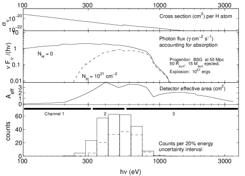
Figure 1: Construction of the LOBSTER instrument response to a blue supergiant SN at a distance of $2D_{\rm min}=$ 50 Mpc. Eight events are expected at this distance (Eq. [9]). Top panel: interstellar cross section per H atom (Wilms et al., 2000). Second panel: Blinnikov et al. (2000)’s model for the breakout flash of SN 1987A, scaled with MM 99’s scaling relations (solid) and extincted by a typical column (dashed). Third panel: LOBSTER effective area. Bottom panel: counts for the unextincted (solid) and extincted (dashed) flash, binned in 20% bins (the energy uncertainty of the detector). Also shown are the three energy channels we use to characterize colour.

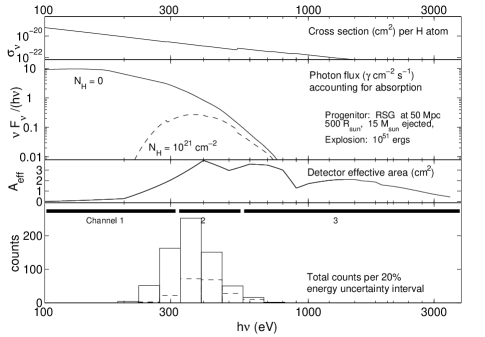
Figure 2: As in Figure 1, but for a red supergiant model. The breakout flash was calculated by Blinnikov et al. (1998) for SN 1993J; see §3.2.

The motivation for this choice is twofold. First, there are five desired intrinsic parameters, two of which ($E_{\rm se}$ and $D$) cannot be disentangled without optical followup; therefore only four X-ray observables need be used. Second, if supernovae occur homogeneously within the detection volume, the number of bursts observed scales as the limiting fluence according to $N\propto$(fluence)^-3/2. The median burst fluence is therefore only $60\%$ above the detection threshold, and cannot be described in fine detail.

After describing the LOBSTER instrument (§3.1), we describe our method for simulating X-ray observables (§3.2) and our strategy for constraining supernova parameters with these four observables (§§3.3–3.5).

3.1 Model of the LOBSTER instrument response

Table 2: SN detection distance and rate versus model type. The factor $f_{\rm obs}$ represents the unknown population of each subclass (Eq. [9]). In each model, $M_{\rm ej}=15M_{\sun}$, $E_{\rm in}=10^{51}$ erg, and $\kappa=0.34$ cm² g^-1, unless otherwise noted.

Progenitor	$N_{\rm H}$	$R_{\star}$	$D_{\rm max}$	Detections	Note
Type	($10^{21}$ cm-2)	($R_{\sun}$)	(Mpc)	per year
BSG	1	50	260	$\sim 320f_{\rm obs}$	SN 1987A analogue
BSG	5	50	86	$\sim 12f_{\rm obs}$	SN 1987A analogue
RSG	1	500	420	$\sim 1400f_{\rm obs}$
RSG	5	500	66	$\sim 6f_{\rm obs}$
RSG	1	500	800	$\sim 10000f_{\rm obs}$	SN 1993J analogue; $M_{\rm ej}=2M_{\sun}$
Wolf-Rayet core	1	5	58	$\sim 1f_{\rm obs}$	BSG scaled to SN Type Ib/c analogue;
					$M_{\rm ej}=3M_{\sun}$, $\kappa=0.2$ cm2 g-1, $\rho_{1}/\rho_{\star}=0.1$

LOBSTER is a proposed wide-field soft X-ray detector, currently envisioned to be deployed on the International Space Station in 2009. LOBSTER has a field of view of 162$\times$22.6 degrees and would continually scan the sky as it orbits the Earth every 90 minutes. Doing this, it would image $\;\buildrel>\over{\sim}\;$95% of the sky once every orbit. LOBSTER has a spatial resolution of approximately 4 arcmin, and is sensitive to soft X-rays of energy 0.1 – 3.5 keV from sources with fluxes of order $10^{-12}$ erg cm^-2 s^-1 (Priedhorsky et al., 1996). Incident photon energies are recorded with an accuracy of roughly $20\%$, implying $\sim 19$ effective spectral channels.

LOBSTER focuses X-rays through grazing angle reflections by an array of microchannels. This arrangement produces a cruciform focal spot on the detector, with a bright central focus spot at the intersection of two dimmer, orthogonal arms; there is also a diffuse background of unfocused photons. The instrument’s effective area is a complicated function of incident photon energy, being limited at low energies by detector window absorption and at higher energies by decreased reflectivity. Shown in the third panel of Figure 1 is the effective area for the central focus, from data provided by Nigel Bannister (2003, private communication). For a full discussion, see Priedhorsky et al. (1996).

The instrument’s field of view should allow for successful detection of numerous shock breakouts. One can define the instantaneous volume of view

$$V_{\rm view}=\frac{1}{3}\Omega D_{\rm max}^{3}$$

where $D_{\rm max}$ is the maximum distance at which a certain flash can be detected. The field of view, $\Omega$, is a narrow swath of the celestial sphere: $\Omega=2(162^{\circ})\sin(22.6^{\circ}/2)=1.11$ sr.

The instantaneous volume of view is appropriate for events that are shorter than the dwell time $t_{\rm dwell}$ of the experiment. The dwell time for LOBSTER has a minimum value of roughly (90 min)(22.6^∘ /360^∘) = 340 s, with longer times occurring near the poles of the orbit, to a maximum of $t_{\rm dwell}=1800$ s (Bannister, 2003). We will adopt the typical value of 400 s for $t_{\rm dwell}$. Longer events can be found even if their beginnings are not observed, leading to a larger effective solid angle $\Omega_{\rm eff}\simeq(1+t/t_{\rm dwell})\Omega$, until the event is viewed in more than one scan of the sky (although this is not expected for breakout flashes). This increase in sensitivity for long events comes at a cost: the burst duration $t$ is no longer directly observable, and can only be constrained.

Note that Klein & Chevalier (1978) assumed that breakout flashes would outlast the 30 s dwell time of HEAO 1, and calculated their detection rate accordingly. LOBSTER’s dwell time, in contrast, is an order of magnitude longer; only RSGs (with $R_{\star}>170R_{\sun}$) have $t>t_{\rm dwell}$ for this experiment.

Cappellaro et al. (1999) quote a rate of $0.71h^{2}$ Type II supernovae per century per $10^{10}$ solar luminosities in the B band. There are $2\times 10^{8}hL_{\odot}{\rm Mpc}^{-3}$ in the B band (Fukugita et al., 1998); from Spergel et al. (2003) we adopt $h=0.71$ (the Hubble constant in units $100\,\rm km\,s^{-1}\,Mpc^{-1}$).

If a fraction $f_{\rm obs}$ of Type II supernovae belong to a subclass of interest, and if this subclass is observable to distance $D_{\rm max}$, then the number of flashes of this type expected in the total integration time of the instrument’s life, $t_{\rm obs}$, is

$$N_{\rm obs}=f_{\rm obs}\left[\frac{D_{\rm max}}{D_{\rm min}(t_{\rm obs})}\right]^{3}.$$ (9)

The quantity $D_{\rm min}(t_{\rm obs})$, a function of the duration of the experiment, is the minimum distance at which one would expect, statistically, to observe one SN II of any progenitor type:

$$D_{\rm min}(t_{\rm obs})=26\left[\frac{3\,\rm yr}{t_{\rm obs}}\left(\frac{t_{\rm dwell}}{t+t_{\rm dwell}}\right)\right]^{1/3}{\rm Mpc}.$$ (10)

Although this is comparable to the distance to the Virgo cluster, the universe is reasonably homogeneous on scales $D>D_{\rm min}$. (The local overdensity may reduce the actual minimum distance by $\sim 25\%$ relative to $D_{\rm min}$; however we neglect this effect in its definition.)

For the LOBSTER mission, $t_{\rm obs}\approx 3$ years; Table 2 shows $D_{\rm max}$ and $N_{\rm obs}$ for various progenitor types, including the canonical SNe II (a RSG progenitor with $M_{\rm ej}=15M_{\sun}$, $R_{\star}=500R_{\sun}$, $E_{\rm in}=10^{51}$ erg, and a BSG progenitor with $M_{\rm ej}=15M_{\sun}$, $R_{\star}=50R_{\sun}$, $E_{\rm in}=10^{51}$ erg). Although the number of events observed depends strongly on parameters, LOBSTER should observe between $\sim 10^{2}$ and $10^{3}$ SNe II and of order one SN Ib/c over a three year lifespan. In §3.2.1 we refine these estimates by averaging over the distribution of absorbing columns $N_{\rm H}$; see Figure 3 and Table 4.

Note that in Table 2 we have included Type Ib/c supernovae, which occur five times less frequently than Type IIs (Cappellaro et al., 1999) and hence have $D_{\rm max}=44$ Mpc. Their observability is rather strongly dependent on the rather poorly known initial radius, ejected mass, and explosion energy: for these events, $N_{\rm obs}\propto(E_{\rm se}/T_{\rm se})^{3/2}\propto E_{\rm in}^{0.4}M_{\rm ej}^{-0.4}R_{\star}^{2}$ (quite approximately, because $A_{\rm eff}(h\nu)$ is not flat and extinction is not completely negligible). In the table, we denote by $f_{\rm obs}$ an unknown fraction with the properties given in Table 2.

3.2 Prediction of Breakout Flash Properties

We describe in this section the prediction of X-ray observables from the properties of a model explosion. We begin by calculating the intrinsic parameters $E_{\rm se}$, $T_{\rm se}$, and $t_{\rm se}$ using the equations presented by MM 99 as shown in Table 1. We choose from the literature a numerical calculation of the breakout spectrum as close as possible to the desired explosion, then shift the spectrum to make its total energy and mean photon energy conform to these model predictions.

Unfortunately, there are very few published calculations of breakout flashes. For red supergiants there is the calculation by Klein & Chevalier (1978), and the more recent model for SN 1993J (Blinnikov et al., 1998). Klein & Chevalier’s model includes a hard tail of higher-energy photons that is absent in Blinnikov et al.’s model, presumably due to the more sophisticated radiation transfer employed in the latter. Because Blinnikov et al. (1998) employ multi-group transfer calculations, we adopt this calculation as the fiducial RSG flash. However, there is insufficient information about the progenitor in the literature to calculate $T_{\rm se}$ for it using the MM 99 equations. When using it, therefore, we enforce that the mean photon energy agrees with the value $2.7kT_{\rm se}$ appropriate for a blackbody of that colour temperature.

For blue supergiants there are two potential sources of breakout spectra: Ensman & Burrows (1992) and Blinnikov et al. (2000), both of which were calculated for SN 1987A. We use the latter, again because the multigroup radiation transfer method employed therein is the more sophisticated. In this case the MM 99 formulae could be applied to the progenitor model, and predict, within 20%, the mean photon energy. We nevertheless enforce a mean energy of $2.7kT_{\rm se}$ when constructing model BSG flashes, to be consistent with the RSG case.

For all Type II supernovae we fixed $f\kappa$ at 0.34 cm² g^-1 (§2).

Table 3: Parameters used in scaling breakout spectra.

Progenitor	$M_{\rm ej}(M_{\sun})$	$R_{\star}(R_{\sun})$	$\rho_{1}/\rho_{\star}$
type
BSG	$1$ – $35$	$20$ – $100$	$0.2$
RSG	$1$ – $35$	$50$ – $1000$	$0.5$

Our three spectral channels were defined as follows: 0.10 – 0.33 keV (channel 1), 0.33 – 0.54 keV (channel 2), and 0.54 – 3.5 keV (channel 3). The chosen energy range matches the response of the LOBSTER instrument, 0.1 – 3.5 keV (§3.1, Figs. 1 and 2). The lower bound of channel 2 was chosen such that all flashes had sufficient channel 1 photons at $D=D_{\min}$ after suffering the expected amount of interstellar extinction ($N_{\rm H}\sim 10^{21}$ cm^-2); the upper bound was set so that all RSG flashes had at least some channel 3 photons prior to extinction.

If $C_{1,2,3}$ are the counts in the three channels, we may define colour parameters $C_{2-1}=\log_{10}(C_{2}/C_{1})$ and $C_{3-2}=\log_{10}(C_{3}/C_{2})$. In the absence of an independent distance determination (see the introduction to §3), these two colour parameters and the flash duration $t$ are the only constraints on the explosion itself. Unlike $t$, $C_{2-1}$ and $C_{3-2}$ are affected by absorption.

Figures 1 and 2 illustrate the prediction of the LOBSTER instrument response to typical blue and red supergiant explosions, respectively.

3.2.1 Interstellar X-Ray Absorption

Table 4: SN detection rate averaged over a distribution of extinctions. SN models from Table 2, the Galactic column density distribution (Schlegel, Finkbeiner, & Davis, 1998) and an estimate of the extragalactic column distribution (Fig. 4 of Cappellaro et al. 1997) are used to find the typical distance (Eq. 11) observable number, and column density (averaged over observable flashes, Eq. 12) toward each type; see Fig. 3. These are sensitive to the small-$N_{\rm H}$ tail of the extragalactic column distribution, which we reiterate is quite uncertain; see Figure 3.

Type	$R_{\star}$	$\left<D_{\rm max}^{3}\right>^{1/3}$	Detections	$\left<\log_{10}N_{\rm H}({\rm cm}^{-2})\right>$
	($R_{\sun}$)	(Mpc)	per year
BSG (87A analogue)	50	96	$17f_{\rm obs}$	21.40
RSG	500	113	$27f_{\rm obs}$	21.32
RSG (93J analogue)	500	223	$210f_{\rm obs}$	21.33
W-R core (Ib/c)	5	37	$0.2f_{\rm obs}$	21.68

In the X-ray, bound-free absorption by the interstellar medium (ISM) is greatest for the softest photons. This leads to a “bluening” of the X-ray spectrum as opposed to reddening in the optical. To account for the effects of absorption, we apply the X-ray opacities of Wilms et al. (2000) and consider a range of hydrogen column densities $N_{\rm H}$. Milky Way columns (Schlegel, Finkbeiner, & Davis, 1998) can roughly be described with a log-normal distribution: $\log_{10}(N_{\rm H}/{\rm cm}^{-2})\simeq 10^{20.72\pm 0.62}$ (1$\sigma$ error bars).

Host galaxy column densities toward Type II and Type Ib/c supernovae are quite uncertain; however there is evidence they are often significantly larger than typical Milky Way columns. Cappellaro et al. (1997) estimate blue magnitudes of extinction toward SNe of both types by searching for trends with galaxy inclination (after accounting for the type of the host and adopting a fiducial value for the face-on extinction). Adopting the model plotted in their Figure 4 leads to a range of $N_{\rm H}$ from $1.5\times 10^{21}$ cm^-2 to $1.3\times 10^{22}$ cm^-2, in a distribution strongly skewed toward higher values.

These are comparable to the columns through Galactic molecular clouds, which may reflect the interstellar context in which they explode. On the other hand, molecular gas is seen to disperse from OB associations on timescales shorter than the typical presupernova lifetime (Blaauw, 1991). Moreover, van den Bergh (1991) argues that chimneys around OB associations produce an observed bias toward face-on galaxies. In these two ways, energetic feedback from OB stars may reduce $N_{\rm H}$ in a fraction of the supernova population.

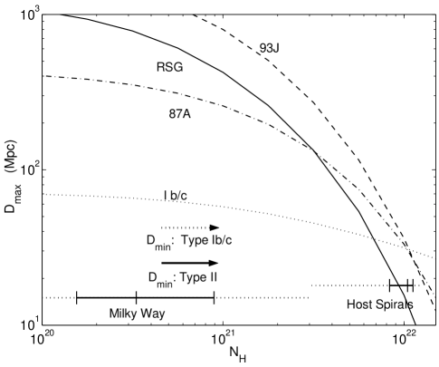
Figure 3: Maximum distance of observability, $D_{\rm max}$, versus absorbing column $N_{\rm H}$ for several progenitor models. Models with harder spectra are less sensitive to extinction. Also plotted are the distances $D_{\rm min}$ within which one supernova is expected in three years; one expects $\sim D_{\rm max}^{3}/D_{\rm min}^{3}$ events. The distribution of columns due to the Milky Way (Schlegel, Finkbeiner, & Davis, 1998) and inferred for host spiral galaxies Cappellaro et al. (1997) are shown (dotted lines: 10th to 90th percentiles; solid dashes: 25th, 50th, and 75th percentiles). Note that the host column distribution is very uncertain.

The Galactic and extragalactic column distributions are shown in Figure 3. Since $N_{\rm obs}\simeq D_{\rm max}^{3}/D_{\rm min}^{3}$, it is quite clear that the statistics of the LOBSTER breakout-flash catalogue will be sensitive to the low-$N_{\rm H}$ end of the host-galaxy column distribution. This is demonstrated in Table 4, which gives the effective value of $D_{\rm max}$ averaged over the extinction distribution:

$$\langle D_{\rm max}^{3}\rangle\equiv\int D_{\rm max}(N_{H})^{3}\frac{d{\cal P}(<N_{\rm H})}{dN_{\rm H}}dN_{\rm H},$$ (11)

where ${\cal P}(<N_{\rm H})$ is the probability that the column density is less than $N_{\rm H}$. The expected number is then $N_{\rm obs}=f_{\rm obs}\langle D_{\rm max}^{3}\rangle/D_{\rm min}^{3}$ as in Eq. (9).

Table 4 also gives the log-normal value of $N_{\rm H}$, averaged over the observed bursts:

$$\langle\log_{10}N_{\rm H}\rangle\equiv\frac{\int D_{\rm max}(N_{H})^{3}\frac{d{\cal P}(<N_{\rm H})}{dN_{\rm H}}\left(\log_{10}N_{\rm H}\right)dN_{\rm H}}{\int D_{\rm max}(N_{H})^{3}\frac{d{\cal P}(<N_{\rm H})}{dN_{\rm H}}dN_{\rm H}}.$$ (12)

Although these numbers are subject to our uncertainty of ${\cal P}(<N_{\rm H})$, they give a sense of what may realistically be observed in a survey. Both estimates strongly weight the low end of the $N_{\rm H}$ distribution, causing the ‘typical’ column to be only $\sim 2-2.5\times 10^{21}$ cm^-2.

The stellar wind of the progenitor star can have a column far in excess of the interstellar values: for a mass loss rate $\sim 10^{-5}M_{\sun}/$yr and a terminal velocity of order the escape velocity, it is $\sim 2\times 10^{23}(10M_{\sun}/M_{\star})^{1/2}(50R_{\sun}/R_{\star})^{1/2}{\rm cm^{-2}}$. However, this wind is fully ionized by a small fraction of the breakout photons (see Lundqvist & Fransson, 1988) and cannot significantly affect the X-ray spectrum.

The closest supernova expected in the LOBSTER catalogue is located $D_{\rm min}\approx 26$ Mpc away, as defined in equation (9) assuming three years of observation (RSGs with $t>t_{\rm dwell}$ should be detected at a shorter distance; §3.1). If the total number of counts detected from a supernova at $D_{\rm min}$ is less than 10 (a fiducial number), we consider the supernova unobservable. (Unobservable flashes have $D_{\rm max}<D_{\rm min}$.) Likewise, we consider the colour parameters $C_{2-1}$ and $C_{3-2}$ uncharacterized if there are not enough counts ($<5$ in a necessary channel) to construct them given a SN at $D_{\rm min}$. These definitions are employed in Figures 4, 5, 6, and 7 to identify excessive values of $N_{\rm H}$.

When the effective area of the LOBSTER instrument is taken into account, analysis reveals that all BSG and RSG progenitor models with $E_{\rm in}=10^{51}$ erg are unobservable when $N_{\rm H}>10^{22}$ cm^-2. The colour parameter $C_{2-1}$ is uncharacterized for all models when $N_{\rm H}>2\times 10^{21}$ cm^-2 and $C_{3-2}$ is uncharacterized when $N_{\rm H}>8\times 10^{21}$ cm^-2.

3.3 Constraints From Timing Alone

It is possible to place constraints on the progenitor radius simply by measuring the duration of the shock breakout burst and comparing the light travel time to the diffusion time for the given range of parameters in Table 3.

One can define a zone of transition from light travel time dominated flashes to those dominated by diffusion. By setting $t_{c}=t_{\rm se}$ and solving for $R_{\star}$, one obtains an expression for the radius of a RSG progenitor which is in the transition zone ($R_{\star\rm TZ}$):

$$R_{\star\rm TZ} = 697\left(\frac{f\kappa}{0.34{\rm cm}^{2}{\rm g}^{-1}}\right)^{0.50}\left(\frac{\rho_{1}}{\rho_{\star}}\right)^{0.24}$$ (13)

$$\times \left(\frac{E_{\rm in}}{10^{51}{\rm erg}}\right)^{0.68}\left(\frac{M_{\rm ej}}{10M_{\sun}}\right)^{-0.18}{R_{\sun}}.$$

The duration of a flash from a transition zone supernova ($t_{\rm TZ}$) is simply $R_{\star\rm TZ}/c$:

$$t_{\rm TZ} = 27.0\left(\frac{f\kappa}{0.34{\rm cm}^{2}{\rm g}^{-1}}\right)^{0.50}\left(\frac{\rho_{1}}{\rho_{\star}}\right)^{0.24}$$ (14)

$$\times \left(\frac{E_{\rm in}}{10^{51}{\rm erg}}\right)^{0.68}\left(\frac{M_{\rm ej}}{10M_{\sun}}\right)^{-0.18}{\rm min},$$

slightly longer than the LOBSTER dwell time.

Hence, for breakout bursts with duration $t<t_{\rm TZ}$, the progenitor radius is $ct$, and for those with longer duration, $R_{\star}$ can be constrained via the $t_{\rm se}$ definition of MM 99. Similar equations can be derived to define the transition zone for BSG progenitors, though it should be noted that, for the parameters considered (Table 3), the breakout flashes from BSGs are always light travel time dominated when $E_{\rm in}\lower 2.15277pt\hbox{$\;\buildrel>\over{\sim}\;$}10^{51}$ erg; hence, a transition zone exists only for BSG explosions with less than this canonical energy.

As an example, consider a supernova with $E_{\rm in}=10^{51}$ erg which produces a breakout flash with a well-measured duration $t$. Using the parameters given in Table 3 and equation 14, one can establish minimum and maximum values for the light travel and diffusion times of RSG and BSG progenitors and draw conclusions from how $t$ falls into these ranges. If $t<116$ s, the progenitor is a BSG and its radius is $ct$ (since no RSG progenitor has such a small light travel time). For a duration of 116 – 230 s, the colour of the flash could be used to distinguish between RSG and BSG (see §3.4), and the progenitor radius is $ct$ (since both RSGs and BSGs can have a $t_{c}$ of this magnitude). A flash $>230$ s long denotes a RSG (since no BSG is large enough to produce a flash this long); for 230 s $<t<$ 1100 s the radius is $ct$ (since the minimum value of $t_{\rm TZ}$ is 1100 s), and for $t>2080$ s restrictions can be placed on $R_{\star}$ using the equation for $t_{\rm se}$. Flashes with duration 1100 – 2080 s are RSG type and could be either $t_{c}$ or $t_{\rm se}$ dominated (since the maximum value of $t_{\rm TZ}$ is 2080 s). Note, however, that the duration of a flash is not well constrained by LOBSTER if it exceeds the $\sim 400$ s dwell time of the experiment.

These results are summarized in Table 5.

Table 5: Constraints on progenitor type and $R_{\star}$ from timing alone. An explosion energy $E_{\rm in}=10^{51}$ erg is assumed. Note that 1100 – 2080 s is the region spanned by the transition zone (TZ); hence, a breakout flash with this duration could be either $t_{c}$ or $t_{\rm se}$ dominated – more information is required.

$t$ (s)	Progenitor	$R_{\star}$
	type
$0$ – $116$	BSG	$ct$
$116$ – $230$	need colour info	$ct$
$230$ – $1100$	RSG	$ct$
$1100$ – $2080$	RSG	near TZ
$>2080$	RSG	can constrain using $t_{\rm se}$

3.4 Constraints From Timing and Colour

By considering the colour of a flash in addition to its duration, more information about the supernova can be deduced and certain degeneracies may be broken. For instance, a flash with duration 116 s $<t<$ 230 s (from a $10^{51}$ erg supernova) is light travel time dominated, but both large BSGs and small RSGs produce flashes of such duration. The colour of the flash may help to break this degeneracy and allow for an identification of the progenitor type.

$T_{\rm se}$ varies inversely with $R_{\star}$; hence, larger progenitors produce redder flashes of lower radiation temperature with more channel 1 photons than smaller progenitors do. As can be seen in Figure 4, a RSG produces a flash which is distinctly bluer in colour than that of a BSG of the same radius (same flash duration); however, RSG flashes in general are redder and brighter since RSGs typically have much larger radii than BSGs. The colour difference between BSG and RSG flashes of the same radius is enhanced by increasing the absorbing column density, as the redder BSG flashes lose proportionally more channel 3 counts than their RSG counterparts (this effect is evidenced by the divergence of the two types in $C_{3-2}$ space). Figure 5 shows that RSG and BSG flashes lose proportionally the same amount of counts in channels 1 and 2 as absorption increases (no divergence). It seems unlikely that the “type degeneracy” mentioned in §3.3 can be broken without an estimate for $N_{\rm H}$ and an accurate measure of the flash colour.

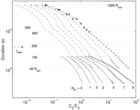
Figure 4: Duration and $C_{3-2}$ colour index for all progenitor models; the solid line indicates BSGs and the dashed line RSGs. Each curve corresponds to a value of $N_{\rm H}$, which increases to the right in units of $10^{21}$ cm^-2 as indicated. Dotted lines mark constant radius. Models marked with “x” are uncharacterized and those with “$\circ$” are unobservable (§3.2.1). The discontinuity in slope in the RSG plot denotes the transition from light travel time to diffusion time in the burst duration. Note that lines of constant radius for $t>t_{\rm TZ}$ are horizontal only because $M_{\rm ej}$ and $E_{\rm in}$ are held constant in each model at $15M_{\sun}$ and $10^{51}$ erg, respectively.

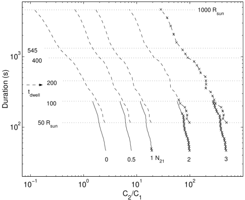
Figure 5: Duration and $C_{2-1}$ colour index for all progenitor models; the solid line indicates BSGs and the dashed line RSGs. Each curve corresponds to a value of $N_{\rm H}$, which increases to the right in units of $10^{21}$ cm^-2 as indicated. Dotted lines mark constant radius. Points marked with “x” indicate models which are uncharacterized (§3.2.1). The discontinuity in curvature of the RSG plot denotes the transition from $t_{c}$-dominated to $t_{\rm se}$-dominated duration. Note that lines of constant radius for $t>t_{\rm TZ}$ are horizontal only because $M_{\rm ej}$ and $E_{\rm in}$ are held constant in each model at $15M_{\sun}$ and $10^{51}$ erg, respectively.

As previously noted, increased absorption causes the values of $C_{2-1}$ and $C_{3-2}$ to increase as lower energy photons are preferentially absorbed. A greater $E_{\rm in}$ also leads to increased colour values due to its proportionality with $T_{\rm se}$, whereas $M_{\rm ej}$ is inversely proportional to the radiation temperature (c.f. Table 1). The effect of $E_{\rm in}$ on colour is very small ($\sim 0.2$ power-law dependence) compared to that of $N_{\rm H}$ (exponential dependence), and the effect of $M_{\rm ej}$ is minute ($\sim-0.05$ power law dependence); $E_{\rm in}$ and $M_{\rm ej}$ do have a significant effect on $t_{\rm se}$. In the case of bursts with $t>t_{\rm dwell}$, whose durations cannot be determined by LOBSTER , the SN properties are best constrained using flash luminosity and colour (§3.5).

Accurate observations of a flash’s duration and colour can pinpoint the location of the flash on a $t$ vs. $C_{3-2}$ or $t$ vs. $C_{2-1}$ plot (Fig. 4 or 5) and hence constrain the value of $N_{\rm H}$ in addition to $R$. If $N_{\rm H}$ is known from other observations, it can be used in tandem with LOBSTER colour observations to constrain $M_{\rm ej}$ and $E_{\rm in}$.

Potentially better constraints come from a colour-colour diagram. Figure 6 shows that the bluening effect of extinction can, to some extent, be disentangled from the intrinsic flash colour to provide an estimate of both $N_{\rm H}$ and $T_{\rm se}$. The latter can then be taken as a constraint on $E_{\rm in}$, $M_{\rm ej}$, and $R_{\star}$, which is significantly more illuminating if $R_{\star}$ is constrained by other means. If, in addition, $E_{\rm se}/t$ is determined by comparing the observed count rate to a value of $D$ (from optical followup; Figs. 7 and 8; §3.5), then all explosion parameters are constrained.

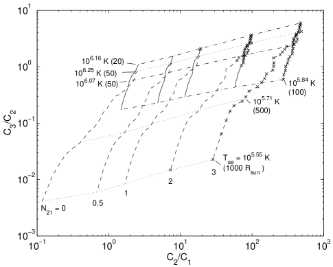
Figure 6: Colour-colour plot for all progenitor models; the solid line indicates BSGs and the dashed line RSGs. Each solid or dashed curve corresponds to a value of $N_{\rm H}$, which increases to the right in units of $10^{21}$ cm^-2 as indicated. Dash-dotted lines mark constant colour temperature $T_{\rm se}$ for BSG models, dotted lines mark constant $T_{\rm se}$ for RSG models. With each $T_{\rm se}$ is provided (in parentheses) the value of $R_{\star}$ at which this value is attained in the case $E_{\rm in}=10^{51}$ erg and $M_{\rm ej}=15M_{\sun}$. Points marked with “x” indicate models which are uncharacterized (§3.2.1).

3.5 Constraints from Luminosity and Colour

Flashes that outlast the LOBSTER dwell time have durations that can only be constrained rather than measured; this puts a lower limit of roughly 170 $R_{\sun}$ on the progenitor. Their durations may be either diffusion or light travel-time dominated (§2), but equation (6) is unlikely to discriminate between these possibilities with only a lower bound on $t_{\rm se}$.

The readily observable quantities for these long bursts are their X-ray colours and brightnesses. We will assume that optical follow-up allows a determination of flash distances: in that case, one can construct an X-ray Hertzsprung-Russell (H-R) diagram for them (Figure 7). In the H-R diagram, the rate of observable photon production ($4\pi D^{2}$ [Count rate]) is plotted versus a colour index. Specifying $T_{\rm se}$, $E_{\rm se}/t$, and $N_{\rm H}$ produces a point on the plot. We hold $E_{\rm se}/t$ constant and vary $T_{\rm se}$ and $N_{\rm H}$ to illustrate trends; varying $E_{\rm se}/t$ simply results in a vertical shift of the curves.

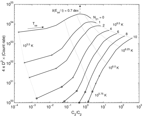
Figure 7: A theoretical X-ray Hertzsprung-Russell diagram of breakout flashes, in which luminosity (measured via the rate of observable photon production) and colour (here $C_{3-2}$) are compared for RSG models. These quantities are observable even if the burst is not viewed for its entire duration, and thus are useful for flashes with $t>t_{\rm dwell}$. Each curve corresponds to a value of $N_{\rm H}$, which increases in units of $10^{21}$ cm^-2 as indicated. Dotted lines mark constant values of $T_{\rm se}$ as indicated; $T_{\rm se}$ increases to the right along each curve. All models are evaluated at constant $E_{\rm se}/t$ ($10^{45}$ erg/s); a change in $E_{\rm se}/t$ results in a vertical shift of the curves (the dashed arrows shows a 0.9 dex shift). Models marked with “x” are uncharacterized and those with “$\circ$” are unobservable (§3.2.1).

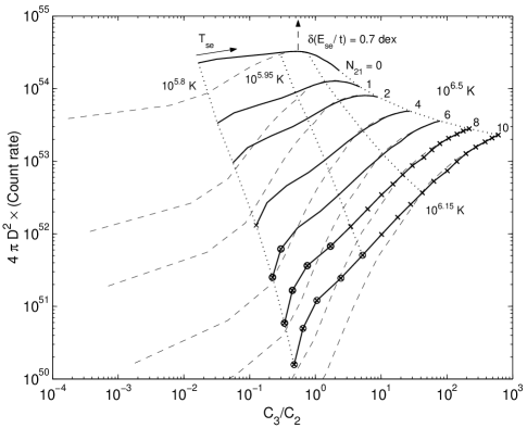
Figure 8: As in fig. 7, but for BSG models (thick solid lines). RSG models appear as thin dashed lines for comparison. These quantities are observable even if the burst is not viewed for its entire duration, although all BSG progenitors are expected to have duration $t<t_{\rm dwell}$. Each curve corresponds to a value of $N_{\rm H}$, which increases in units of $10^{21}$ cm^-2 as indicated. Dotted lines mark constant values of $T_{\rm se}$ as indicated; $T_{\rm se}$ increases to the right along each curve. All models are evaluated at constant $E_{\rm se}/t$ ($10^{45}$ erg/s); a change in $E_{\rm se}/t$ results in a vertical shift of the curves (the dashed arrows shows a 0.9 dex shift). Models marked with “x” are uncharacterized and those with “$\circ$” are unobservable (§3.2.1).

By placing a point on Figure 7 representing the observed characteristics of a flash, it possible to fix $T_{\rm se}$. With other information, such as that provided by the colour-colour diagram (Fig. 6), $N_{\rm H}$ and $E_{\rm se}/t$ can be constrained. Through the scaling equations (1), $M_{\rm ej}$, $E_{\rm in}$, and $R_{\star}$ can, in turn, be constrained. Although all BSG progenitors are expected to produce flashes with $t<t_{\rm dwell}$, we include an H-R diagram for BSGs for the purposes of comparison (Fig. 8). For higher $T_{\rm se}$ models, BSG flashes are effectively indistinguishable from RSG flashes of the same flash luminosity, $E_{\rm se}/t$. The H-R diagram does not present a good means of constraining progenitor type for flashes with $t<t_{\rm dwell}$; the other methods described in this section work best. For long flashes which are not observed in their entirety, the H-R diagram could prove invaluable.

4 Shock travel time

The travel time for the shockwave responsible for the breakout flash, or equivalently, the time lag between the emergence of neutrinos and gravity waves from the exploding star and the emergence of shock breakout, is well approximated by

$$\Delta t_{\nu,\gamma} = \int_{0}^{R_{\star}}\frac{dr}{v_{s}}$$

$$= 1.26\frac{R_{\star}M_{\rm ej}^{1/2}}{E_{\rm in}^{1/2}}\int_{0}^{1}\left[\frac{m(r)}{M_{\rm ej}}\right]^{1/2}\left[\frac{\rho_{0}(r)r^{3}}{m(r)}\right]^{0.19}\frac{dr}{R_{\star}}.$$

Stellar mass and density profiles are needed to define $v_{s}$ (Eq. 3); the authors used progenitor structures provided by Woosley and Nomoto. For a $16M_{\sun}$, $48R_{\sun}$ BSG with $M_{\rm ej}=14M_{\sun}$ and $E_{\rm in}=10^{51}$ erg, $\Delta t_{\nu,\gamma}$ is 2 hours. For an $18M_{\sun}$, $450R_{\sun}$ RSG with $M_{\rm ej}=16.5M_{\sun}$ and $E_{\rm in}=1.1\times 10^{51}$ erg, the delay between neutrino/gravity wave emission and shock breakout is 36 hours. It should be noted that this method to determine the time of shock emergence using equation (4) is considerably more accurate than the Sedov solution for a constant density envelope, used by Woosley et al. (2002) and others. The determination of $\Delta t_{\nu,\gamma}$ is not of consequence observationally unless the supernova in question occurs within a few kpc; in this case, it is feasible to detect the neutrino/gravity wave emission with the appropriate detectors. Near-future gravity wave detectors will only be able to detect SNe within our Galaxy (Ott et al., 2004), whereas neutrino signals can be detected out to the Magellanic clouds. Neutrino and/or gravity wave detection would provide: 1. early warning that a breakout flash (and supernova) will occur, and 2. a measurement of $\Delta t_{\nu,\gamma}$, which could be used to further constrain the supernova properties. It should be noted, however, that the rate for Galactic supernovae is very low ($\sim 0.01$ yr^-1), that only $\sim 9\%$ of these fall within the LOBSTER field of view, and that most of these occur in the Galactic disk, where $N_{\rm H}>10^{22}$ cm^-2 typically; hence, constraining SNe properties using shock travel time could only be done under very fortuitous circumstances.

5 Shock breakout observation with other instruments

In examining the capabilities of an instrument to observe the shock breakout flash, this paper has focused on the proposed LOBSTER wide-field X-ray detector; however, breakout flashes are also detectable by other current instruments – though less frequently and in less detail. Preliminary work by the authors indicates that the EPIC-PN instrument of the XMM-Newton X-ray space observatory, with a narrower field of view but much higher effective area than LOBSTER, is capable of detecting flashes at moderate redshifts. The $\sim 0.2$ deg² field of view increases $D_{\rm min}$ (§3.1), or equivalently, $z_{\rm min}$, to $z_{\rm min}=0.2$; but the high effective area allows detections of the canonical flashes to $z_{\rm max}\sim 0.9$ (c.f. $D_{\rm max}$, §3.1). The Chandra X-ray observatory’s HRC-I has a similar field of view, and hence $z_{\rm min}$, as XMM Newton, with a lower effective area and correspondingly lower $z_{\rm max}\sim 0.2$. The PSPC instrument on the ROSAT satellite, with a large field of view and intermediate effective area, has $z_{\rm min}=0.1$, $z_{\rm max}\sim 0.6$. The assumed columns are $N_{\rm H}=2\times 10^{21}$ cm^-2 in the host galaxy and $N_{\rm H}=0.5\times 10^{21}$ cm^-2 locally. These results indicate that there may be a number of undiscovered breakout flashes in the backgrounds of archived XMM Newton and ROSAT images, of order 10 for each instrument. In the HRC-I images, there may be of order 1 BSG breakout flash and likely none from RSGs; it should be noted that Race et al. (2003) have come to a similar conclusion with regard to the ACIS instrument on Chandra.

Because the breakout flash durations are much shorter than the typical integration times for these instruments, and because a typical flash detection would be dimmer than the X-ray sources observed, the probability of a serendipitous discovery is almost zero. This may explain why the archived breakout flashes have gone unnoticed, even if present in the data. An in-depth search of the archived images would be required to locate the detected flashes.

A sensitive optical survey with a sufficiently large field of view may be able to detect the Rayleigh-Jeans tail of the breakout flash spectrum. Preliminary calculations indicate that, to an extinctionless limiting magnitude of $\sim 23$ mag in both the U and B bands (Johnson-Morgan system), there is one flash per square degree per $200f_{\rm obs}^{-1}$ years for the canonical RSG, and one flash per square degree per $600f_{\rm obs}^{-1}$ years for the canonical BSG. Extinction in the host galaxy typically causes the limiting magnitude to increase to $\sim 24$ mag.

We have ruled out the possibility of detecting high redshift breakout flashes with optical telescopes; the high luminosity distances involved more than compensate for the cosmological K-correction.

6 Discussion

We have combined an analytical theory for the dependence of shock breakout parameters (MM 99) with numerical simulations of shock breakout flashes (Klein & Chevalier, 1978; Blinnikov et al., 1998; Ensman & Burrows, 1992; Blinnikov et al., 2000) to predict the expected signal observed by the LOBSTER spaceborne soft X-ray camera. Our emphasis has been on the reconstruction of supernova parameters – primarily radius, mass, explosion energy, and obscuring column – from the data (§3).

Supernova radius is the most tightly constrained of the three quantities (§3.3). For all events which have a duration that can be measured individually, because it is shorter than the dwell time of the instrument, the duration is set by the light travel time of the star rather than the leakage of photons from the surface layers of the explosion. These events come from stars with $R\lower 2.15277pt\hbox{$\;\buildrel<\over{\sim}\;$}170R_{\sun}$, i.e., blue supergiants and relatively compact red supergiant progenitors. Such flashes are characteristically harder and dimmer than those from more extended RSG progenitors; nevertheless, they are visible to distances of several hundred Mpc and should be observed in the hundreds per year (Table 2).

For these stars, the flash colour temperature $T_{\rm se}$ and absorbing column $N_{\rm H}$ can be estimated for extinctions $N_{\rm H}\lower 2.15277pt\hbox{$\;\buildrel<\over{\sim}\;$}2\times 10^{21}\ {\rm cm^{-2}}$ by placing them on duration-colour (Figs. 4 and 5) and colour-colour (Fig. 6) diagrams. $T_{\rm se}$ provides a constraint on the explosion energy and ejected mass through the equations derived by MM 99 (Table 1); however, these quantities cannot be derived independently without additional information. In the case that optical followup provides a distance, this degeneracy can be broken (Figure 7).

Events that outlast LOBSTER’s dwell time are overrepresented because they can be detected even if they do not begin while inside the field of view (§3.1). However they are also poorly characterized, because only a lower limit is available for their duration. With optical follow-up they can still be placed on Figure 7, allowing an estimate of the obscuring column and the colour and luminosity of the breakout flash.

6.1 Implications

From the above analysis we draw several conclusions. The LOBSTER space observatory will provide a census of Type II supernova events that is complete within $\sim 250$ Mpc (Table 2 and Figure 3) and up to columns $N_{\rm H}\lower 2.15277pt\hbox{$\;\buildrel>\over{\sim}\;$}10^{21}{\rm cm^{-2}}$. The number of events expected in three years of LOBSTER observations is quite uncertain, but for a conservative estimate of host-galaxy extinction (Table 4) it ranges from $\sim 50$ to $\sim 600$ depending on the typical radius of the progenitor stars.

A population of dim Type II supernovae from blue progenitors is suggested by SN 1987A and its analogues (Schmitz & Gaskel, 1988; Fillipenko, 1988; Young & Branch, 1988; Schaefer, 1996), although its significance is controversial (van den Bergh & McClure, 1989). SN 1987A analogues should appear in the data as flashes whose duration is shorter than the dwell time of the instrument. These events, whose properties are difficult to infer from optical observations due to the contribution of ⁵⁶Co (§1.1), will provide strong constraints on stellar evolution at the point of core collapse.

6.2 Caveats

The current work relies on the extrapolation of breakout flash properties for a variety of stellar progenitors from only a pair of numerical calculations, by means of the analytical scaling relations given by MM 99; see §3.2. It is possible that elements of the radiation dynamics cause the overall shape of the breakout spectrum to change across this range, which would introduce a systematic error into our predictions of X-ray observables. This can only be tested with a more systematic survey of breakout properties, preferably using multigroup radiation hydrodynamics simulations.

One limitation of the MM 99 scaling relations is that they cover only two possible forms of the outer density profile ($\rho\propto{\rm depth}^{n}$): $n=3/2$, representing convective envelopes, and $n=3$, representing radiative envelopes with constant opacity. Other possibilities should be considered. For instance, convection is inefficient near the surfaces of red supergiants, and this effects shock propagation in the outermost layers (as MM 99 noted). A superadiabatic layer has a value of $n$ that is lower than the adiabatic value. On the other hand, the MM 99 analysis and our own investigations show that the detailed structure of the outer envelope plays a rather minor role in the breakout flash intensity, colour, and duration (see also the Appendix).

6.3 Speculation: Asymmetric Explosions

As noted above, the short breakout flashes that fit within the LOBSTER dwell time have durations set by the star’s light travel time. This makes it possible for asymmetries in those explosions to affect the time dependence of their breakout flashes. A spherically symmetric explosion will exhibit a progression in brightness and colour that represents the growth of the emitting area and the change of its limb darkening as the observable portion of the breakout moves from the front to the side of the star (e.g., Ensman & Burrows, 1992). If the explosion is sufficiently asymmetric, then this pattern will be disturbed by the motion of the shock front across the face of the star. Unfortunately, the most compelling evidence would derive from an observation of time-dependent linear polarization of the emerging X-rays; a difficult quantity to observe.

Asymmetries can derive from several sources: asymmetries in the envelope distribution (due to rotation and convective eddies); the growth of (weakly) unstable perturbations in accelerating shocks; and the asymmetry of the central engine driving the explosion, e.g., in the case of a jet-driven explosion. (Note that gamma-ray burst jets are not likely to escape supergiant stars [Matzner 2003]; however they may imprint an asymmetry on the explosions.)

Concentrating on the first of these, how much asymmetry would be required to perturb the shock travel time by an amount comparable to the light travel time? The shock speed is roughly $1(10M_{\sun}/M_{\rm ej})\%$ of $c$ on average, so a relative difference in travel time of the same order is required; this would arise from a comparable asymmetry in the progenitor. This degree of asymmetry may exist in blue supergiants if, for instance, they have undergone tidal interactions with companion stars in previous red supergiant phases or are close to their Roche radii at the time of explosion.

Appendix A Stellar outer density coefficients

The parameter $\rho_{1}/\rho_{\star}$, which describes the density structure of the outermost regions of a progenitor star (§2), appears in the MM 99 equations for the properties of the breakout flash. Though the near-surface structure plays little role in determining the temperature and energy of a breakout flash, it is significant in dictating the duration $t_{\rm se}$ of a diffusion-dominated flash.

The following sections we estimate $\rho_{1}/\rho_{\star}$ for the radiative envelopes of blue supergiants and for the convective envelopes of red supergiants. In each case we motivate replacing $\rho_{1}/\rho_{\star}$ with a particular numerical value; only in exceptionally well-observed breakout flashes could the dependence of $\rho_{1}/\rho_{\star}$ on stellar parameters be used to reconstruct them.

A.1 Outer Density Coefficients for Blue Supergiants

It is possible to re-write the MM 99 scaling equations for BSGs (Table 1) such that $\rho_{1}/\rho_{\star}$ is eliminated in favour of the mass, luminosity, and compositional parameters of the progenitor star. For progenitors with a radiative envelope (i.e., BSGs), $\rho_{1}$ may be expressed as

$$\frac{\rho_{1}}{\rho_{\star}}=\frac{a(\mu m_{H})^{4}}{192k_{B}^{4}}\frac{G^{3}M_{\star}^{3}}{M_{\rm ej}}\frac{\beta^{4}}{1-\beta},$$ (16)

where $1-\beta\equiv L_{\star}/L_{\rm Edd}$ is the ratio of the stellar luminosity to the Eddington limit. For Thompson opacity,

$$1-\beta=0.259\left(\frac{L_{\star}}{10^{5}L_{\odot}}\right)\left(\frac{M_{\star}}{10M_{\odot}}\right)^{-1}\left(\frac{1+X_{H}}{1.7}\right),$$ (17)

which leads to

$$\frac{\rho_{1}}{\rho_{\star}} = 0.571\left(\frac{\mu}{0.62}\right)^{4}\left(\frac{M_{\star}}{10M_{\sun}}\right)^{4}$$ (18)

$$\times \left(1-\frac{L_{\star}}{L_{\rm Edd}}\right)^{4}\left(\frac{M_{\rm ej}}{10M_{\sun}}\right)^{-1}$$

$$\times \left(\frac{L_{\star}}{10^{4}L_{\sun}}\right)^{-1}\left(\frac{1+X_{H}}{1.7}\right)^{-1}.$$

Using theoretical stellar model data from various authors, we have established a semi-empirical mass-luminosity (M-L) relation for presupernova stars. This M-L relation, show in Figure 9, is

$$\frac{L_{\star}}{L_{\sun}}\approx 590\left(\frac{M_{\star}}{M_{\sun}}\right)^{1.95}$$ (19)

and it is valid for the mass range $10<M_{\star}/M_{\sun}<20$. Substituting the M-L relation into equation (18) results in:

$$\frac{\rho_{1}}{\rho_{\star}} = 0.107\left(\frac{\mu}{0.62}\right)^{4}\left(\frac{M_{\star}}{10M_{\sun}}\right)^{2.05}$$ (20)

$$\times \left(1-\frac{L_{\star}}{L_{\rm Edd}}\right)^{4}\left(\frac{M_{\rm ej}}{10M_{\sun}}\right)^{-1}$$

$$\times \left(\frac{1+X_{H}}{1.7}\right)^{-1}.$$

From equation (20) it follows that $\rho_{1}/\rho_{\star}$ varies almost linearly from $\sim 0.13$ to $\sim 0.26$ for $10<M_{\star}/M_{\sun}<20$, assuming a $1.5M_{\sun}$ remnant and $L_{\star}<<L_{\rm Edd}$. Thus, we will adopt the average, $\sim 0.2$, as a fiducial value for all BSG progenitors.

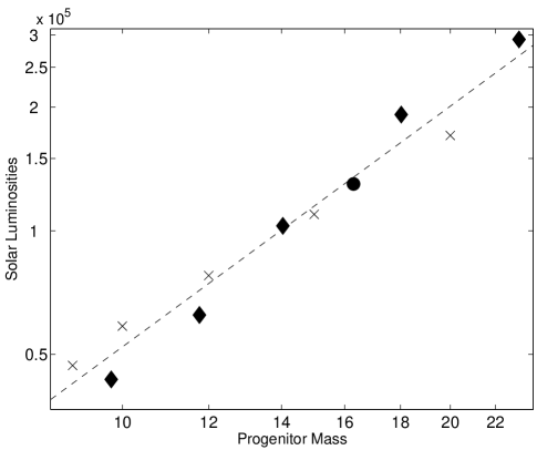
Figure 9: Luminosity-mass relation for presupernova stars. Plotted are the terminal masses and luminosities for the Padova tracks with solar-scaled metallicity $Z=0.008$ (Salachnich et al. 2000, A & A 361, 1023, crosses), for Geneva tracks of the same metallicity (Scherer et al. 1992 A & AS Supp. 98, 523), and for a progenitor model for SN 1987A (Hashimoto, Shigeyama, & Nomoto 1989, circle). Also plotted is a simple power law fit (Eq. 19).

A.2 Outer Density Coefficient for Red Supergiants

Combining equations (9), (14), and (48) from MM 99 results in:

$$\frac{\rho_{1}}{\rho_{\star}}=\left(12.62-12.17q\right)\left(0.37-0.18q+0.096q^{2}\right)^{5/2},$$ (21)

where $q\equiv 1-M_{\rm env}/M_{\star}$ and $M_{\rm env}$ is the mass of the outer stellar envelope. In this case, $\rho_{1}/\rho_{\star}$ exhibits an approximately $1/q$ dependence for the most plausible range of $q$ values, $0.3<q<0.5$ (see Figure 5 of MM 99). For these values of $q$, $\rho_{1}/\rho_{\star}$ varies from $\sim 0.54$ to $\sim 0.33$; we adopt $0.5$ as the standard for RSGs.

Table 6: Alternate scaling equations for progenitors with radiative envelopes, without using the M-L relation. These should be read as exponents in formulae, e.g., $t_{\rm se}=10^{1.65}[f\kappa/(0.34\ {\rm cm^{2}g^{-1}})]^{-0.14}$… cgs units.

Parameter	$T_{\rm se}$	$E_{\rm se}$	$t_{\rm se}$
$10$	$6.11$	$47.37$	$1.65$
$f\kappa/0.34$ cm2 g-1	$-0.14$	$-0.84$	$-0.45$
$E_{\rm in}/10^{51}$ erg	$0.18$	$0.58$	$-0.72$
$M_{\rm ej}/10M_{\sun}$	$-0.11$	$-0.36$	$0.46$
$R_{\star}/50R_{\sun}$	$-0.48$	$1.68$	$1.90$
$M_{\star}/10M_{\sun}$	$0.18$	$-0.22$	$-0.73$
$1-L_{\star}/L_{\rm Edd}$	$0.18$	$-0.22$	$-0.73$
$\mu/0.62$	$0.18$	$-0.22$	$-0.73$
$(1+X_{H})/1.7$	$-0.046$	$0.054$	$0.18$
$L_{\star}/10^{4}L_{\sun}$	$-0.046$	$0.054$	$0.18$

Table 7: Alternate scaling equations for progenitors with radiative envelopes, using the mass-luminosity relation (Eq. [19]). These should be read as exponents in formulae, e,g., $t_{\rm se}=10^{1.78}[f\kappa/(0.34{\rm cm^{2}g^{-1}})]^{-0.45}$… cgs units.

Parameter	$T_{\rm se}$	$E_{\rm se}$	$t_{\rm se}$
$10$	$6.08$	$47.41$	$1.78$
$f\kappa/0.34$ cm2 g-1	$-0.14$	$-0.84$	$-0.45$
$E_{\rm in}/10^{51}$ erg	$0.18$	$0.58$	$-0.72$
$M_{\rm ej}/10M_{\sun}$	$-0.11$	$-0.36$	$0.46$
$R_{\star}/50R_{\sun}$	$-0.48$	$1.68$	$1.90$
$M_{\star}/10M_{\sun}$	$0.10$	$-0.12$	$-0.40$
$1-L_{\star}/L_{\rm Edd}$	$0.18$	$-0.22$	$-0.73$
$\mu/0.62$	$0.18$	$-0.22$	$-0.73$
$(1+X_{H})/1.7$	$-0.046$	$0.054$	$0.18$

References

- Bannister (2003) Bannister, N. 2003, private communication.
- Blinnikov et al. (1998) Blinnikov, S. et al. 1998, ApJ, 496, 454.
- Blinnikov et al. (2000) Blinnikov, S. et al. 2000, ApJ, 532, 1132.
- Blaauw (1991) Blaauw, A. 1991, NATO ASIC Proc. 342: The Physics of Star Formation and Early Stellar Evolution, 125
- Cappellaro et al. (1997) Cappellaro, E. et al. 1997, A&A, 322, 431.
- Cappellaro et al. (1999) Cappellaro, E. et al. 1999, A&A, 351, 459.
- Chevalier (1992) Chevalier, R. A. 1992, ApJ, 394, 599
- Colgate (1968) Colgate, S. A. 1968, Canadian Journal of Physics, 46, 476
- Colgate & White (1966) Colgate, S. A. & White, R. H. 1966, ApJ, 143, 626
- Ensman & Burrows (1992) Ensman, L. & Burrows, A. 1992, ApJ, 393, 742.
- Fillipenko (1988) Fillipenko, A. V. 1988, Supernova 1987A in the Large Magellanic Cloud, 106
- Fukugita et al. (1998) Fukugita, M. et al. 1998, ApJ, 503, 518.
- Gandel’man & Frank-Kamenetsky (1956) Gandel’man, G. M. and Frank-Kamenetsky, D. A. 1956, Sov. Phys. Dokl., 1, 223.
- Grassberg et al. (1971) Grassberg, E. et al. 1971, Ap&SS, 10, 28.
- Grover & Hardy (1966) Grover, R. & Hardy, J. W. 1966, ApJ, 143, 48
- Hamuy (2003) Hamuy, M. 2003, ApJ, 582, 905.
- Iglesias & Rogers (1996) Iglesias, C. A. & Rogers, F. J. 1996, ApJ, 464, 943
- Imshennik & Nadëzhin (1989) Imshennik, V. S. and Nadëzhin, D. K. 1989, Sov. Sci. Rev. E. Astrophys Space Phys, 8, 1.
- Klein & Chevalier (1978) Klein, R. & Chevalier, R. 1978, ApJ, 223, L109.
- Klein et al. (1979) Klein, R. et al. 1979, ApJ, 234, 566.
- Litvinova & Nadëzhin (1985) Litvinova, I. & Nadezhin, D. 1985, Soviet Astron. Lett., 11, 145.
- Lundqvist & Fransson (1988) Lundqvist, P. & Fransson, C. 1988, A&A, 192, 221
- Matzner & McKee (1999) Matzner, C. & McKee, C. 1999, ApJ, 510, 379.
- Matzner (2003) Matzner, C. D. 2003, MNRAS, 345, 575
- Ott et al. (2004) Ott, C. et al. 2004, ApJ, 600, 834.
- Popov (1993) Popov, D. 1993, ApJ, 414, 712.
- Priedhorsky et al. (1996) Priedhorsky, W. et al. 1996, MNRAS, 279, 733.
- Race et al. (2003) Race, D. et al. 2003, AAS Meeting 203, 142.02.
- Sakurai (1960) Sakurai, A. 1960, Comm. Pure Appl. Math., 13, 353.
- Schaefer (1996) Schaefer, B. E. 1996, ApJ, 464, 404
- Schlegel, Finkbeiner, & Davis (1998) Schlegel, D. J., Finkbeiner, D. P., & Davis, M. 1998, ApJ, 500, 525
- Schmitz & Gaskel (1988) Schmitz, M. F. & Gaskel, C. M. 1988, Supernova 1987A in the Large Magellanic Cloud, 112
- Spergel et al. (2003) Spergel, D. N. et.al. 2003, ApJS, 148, 175.
- Stritzinger et al. (2002) Stritzinger, M. et al. 2002, AJ, 124, 2100
- Tan, Matzner, & McKee (2001) Tan, J. C., Matzner, C. D., & McKee, C. F. 2001, ApJ, 551, 946
- van den Bergh (1991) van den Bergh, S. 1991, Proceedings of the Astronomical Society of Australia, 9, 13
- van den Bergh & McClure (1989) van den Bergh, S. & McClure, R. D. 1989, ApJ, 347, L29
- van Dyk et al. (2003) Van Dyk, S. et al. 2003, PASP, 803, 1.
- Wilms et al. (2000) Wilms et al. 2000, ApJ, 542, 914.
- Woosley et al. (2002) Woosley et al. 2002, Rev. Mod. Phys., 74, 1015.
- Young & Branch (1988) Young, T. R. & Branch, D. 1988, Nat, 333, 305