New constraints on the mass composition of cosmic rays above $10^{17}$ eV from Volcano Ranch measurements

Abstract

Linsley used the Volcano Ranch array to collect data on the lateral distribution of showers produced by cosmic rays at energies above $10^{17}$ eV. Very precise measurements of the steepness of the lateral distribution function were made on 366 events. The current availability of sophisticated hadronic interaction models has prompted an interpretation of the measurements. In this analysis we use the aires Monte Carlo code to generate showers, together with geant4 to simulate the detector response to ground particles. The results show that, with the assumption of a bi-modal proton and iron mix, iron is the dominant component of cosmic rays between $5\times 10^{17}$ and $10^{19}$ eV, assuming that hadronic interactions are well-described by qgsjet at this energy range.

PACS: 96.40, 13.85.T High Energy Cosmic rays; mass composition

I Introduction

The measurement of the mass composition of cosmic rays above $10^{17}$ eV is a challenging problem. This information is as important as the energy spectrum and the anisotropy in determining cosmic ray origin. One must know the likely mass range of a particular data set before one can interpret anisotropy information confidently, given the influence of galactic and intergalactic magnetic fields. Our knowledge of the mass composition of cosmic rays above $10^{17}$ eV remains very limited. Recent re-interpretation of measurements of the lateral distribution of water-Čerenkov signals made at Haverah Park  [1] suggests a composition of 34% protons and 66% iron in the range $2\times 10^{17}$ - $10^{18}$ eV. This contrasts with earlier claims, from observations made using Fly’s Eye, that the composition changes from a heavy mix around $3\times 10^{17}$ eV to a proton dominated flux around $10^{19}$ eV [2]. At Yakutsk, both the inferred values of the depth of shower maximum ($X_{max}$) and the muon density favor a composition change from a mixture of heavy and light components to light composition over the same energy region [9]. From HiRes/MIA data [7], there are claims that there is a rapid change from a heavy to a light composition between 0.1 and 1.0 EeV. A recent analysis by the HiRes collaboration of data collected in the energy range between $10^{18}$ - $10^{19.4}$ eV [8] is consistent with a nearly constant purely protonic composition. The fraction of protons, however, decreases when they interpret their data using sibyll2.1. On the other hand, the AGASA group have argued for a “mixed” unchanging composition from 1 - 10 EeV [4] (using mocca for the simulations). A recent analysis of the muon component in air showers with aires/qgsjet98 around $10^{19}$ eV by the AGASA collaboration indicates a relatively light average composition [5].

The source of the discrepancy between different experiments is not understood and it is important to resolve the issue, because of its implications for cosmic ray models of origin, acceleration and propagation. Volcano Ranch data may provide a path for further understanding.

Following the successful re-examination of the Haverah Park data [1] with modern shower models, we report here a similar analysis using the Volcano Ranch data, collected by Linsley [16] to determine the shape of the lateral distribution of air showers. This is the first attempt to examine the Volcano Ranch data with the results of Monte Carlo calculations, using Monte Carlo tools that were unavailable when the data were recorded in 1970. It is timely as the situation on mass composition above $10^{17}$ eV remains confused and the steepness of the lateral distribution is sensitive to the depth of maximum of the shower, and therefore to the primary composition and to the character of the initial hadronic interactions.

To simulate the development of the air showers, we have used the aires [10] code (version 2.4.0), with the hadronic interaction generator qgsjet98 [11]. The results of the simulated showers were convolved with a simulation of the detector response made using geant4 [15]. A comparison of two hadronic generators (qgsjet98 and sibyll2.1 ) was presented in [26]. Both give satisfactory descriptions of the data, but we have preferred to use qgsjet98 because this model has been shown to be consistent with experimental data at energies up to 10 PeV and beyond[13, 14]

II The Volcano Ranch Array

The pioneering Volcano Ranch instrument consisted of an array of scintillation counters. The array was operated in three configurations from 1959-1976 at the MIT Volcano Ranch station located near Albuquerque, New Mexico (atmospheric depth 834 g ${\rm cm^{-2}}$). One of its many distinctions was the detection of the first cosmic ray with an energy estimated at $10^{20}$eV [19]. The final configuration, of relevance here, comprised 80 detectors of surface area 0.815 ${\rm m^{2}}$, scintillator thickness of 9.032 g ${\rm cm^{-2}}$ laid out on a hexagonal grid with a separation of 147 m (Fig1). This configuration allowed precise measurement of the lateral distribution of the detector signals. The steepness of the lateral distribution, and its fluctuations, can be used to explore the primary mass composition as in [1]. Fortunately, in his various writings, Linsley has left unusually detailed descriptions of his equipment, together with examples of events and a description of his data reduction methods.

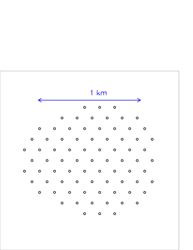
FIG. 1.: Volcano Ranch array in the final configuration.

III Lateral distribution function

A generalized version of the Nishimura-Kamata-Greisen (NKG) formula was used to describe the lateral distribution of particles at ground in minimum ionizing particles per square metre (${\rm mips\,m^{-2}}$) for Volcano Ranch data [24]. This lateral distribution function is given as

$$S_{{\rm VR}}(r)={\frac{N_{fit}}{r_{m}^{2}}}C(\alpha,\eta)\left({\frac{r}{r_{m}}}\right)^{-\alpha}\left(1+{\frac{r}{r_{m}}}\right)^{-(\eta-\alpha)}$$ (1)

normalized to shower size $N_{fit}$ with

$$C={\frac{\Gamma(\eta-\alpha)}{2\pi\Gamma(2-\alpha)\Gamma(\eta-2)}}.$$ (2)

Here $r_{m}$ is the Molière radius, which is $\simeq$ 100 m for the Volcano Ranch elevation. $\eta$ and $\alpha$ are parameters that describe the logarithmic slope of this function.

From a subset of 366 showers detected with the array, the form of $\eta$ as a function of zenith angle $\theta$ and shower size $N_{fit}$ was found to be [20]:

$$\langle\eta(\theta,N_{fit})\rangle=a+b(\sec\theta-1)+c\>log_{10}({\frac{N_{fit}}{10^{8}}})$$ (3)

with $a=3.88\pm 0.054$, $b=-0.64\pm 0.07$, and $c=0.07\pm 0.03$ where a fixed value of $\alpha=1$ was adopted.

IV Simulation of the detector response of the Volcano Ranch array

The aires code provides a realistic air shower simulation system, which includes electromagnetic algorithms [18] and links to different hadronic interactions models. As mentioned above, we have used the qgsjet98 model for nuclear fragmentation and inelastic collisions. For the highest energy showers, the number of secondaries becomes so large that it is prohibitive in computing time and disk space to follow and store all of them. Hillas [17] introduced a non-uniform statistical sampling mechanism which allows reconstruction of the whole extensive air shower from a small but representative fraction of secondaries that are fully tracked. Statistical weights are assigned to the sampled particles to account for the energy of the discarded particles. This technique is known as “statistical thinning”. The aires code includes an extended thinning algorithm, which has been explained in detail [10]. The present work has been carried out using, in most cases, an effective thinning level $\epsilon_{th}=E_{th}/E_{prim}=10^{-7}$ which is sufficient to avoid the generation of spurious fluctuations and to provide a statistically reliable sample of particles far from the shower core. All shower particles with energies above the following thresholds were tracked: 90 keV for photons, 90 keV for electrons and positrons, 10 MeV for muons, 60 MeV for mesons and 120 MeV for nucleons and nuclei.

We have generated a total of 1735 proton and iron showers with zenith angles in the range $\sec{\theta}$ = 1.0 - 1.5 and primary energies between $10^{17}$ eV and $10^{19}$ eV, to match the Volcano Ranch data. To simulate the response of the detectors of the array to the ground particles, we utilized the general-purpose simulation toolkit geant4. Our procedure follows the prescription in [23], where the detector response to electrons, gamma, and muons is simulated in the energy range 0.1 to $10^{5}$ MeV and for five bins per decade of energy. The results of air shower simulations are convolved with the detector response to obtain the scintillator yield expressed in ${\rm mips\ m^{-2}}$. The computed lateral distributions of particles and the corresponding signal from the scintillators for photons, electrons and muons are displayed in Figure 2.

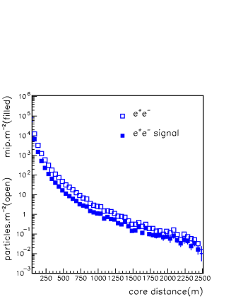
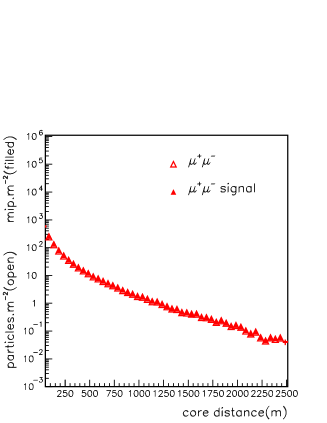
FIG. 2.: Simulated lateral distributions of the three main shower components at ground level and its convolution with the detector response.

A comparison between the lateral distribution measurements[24] and proton/iron showers simulated with aires/qgsjet98 including the scintillator response was presented previously [26]. Each simulated shower was thrown a maximum of 100 times on to the simulated Volcano Ranch array with random core positions in the range 0 - 500 m from the array center.

With the thinning method used in Monte Carlo shower generators, when particles reach the thinning energy just one of them is followed and multiplied by the corresponding weight at the end. Thus, to simulate the response of the detectors correctly, it is necessary to perform a smoothing of the densities of the ground particles around the position of each detector. All particles in a “sampling zone” around a given detector are selected and the statistical weight, as obtained from aires, is multiplied by the “sampling ratio” $A_{detector}/A_{sampling}$ where $A_{sampling}$ is the area of the “sampling zone” and $A_{detector}$ is the corresponding detector area. This is equivalent to sampling particles on a larger area to get a realistic density around the detector position. As the densities depend mainly on the distance to the shower axis, the sampling area over which simulated particles are gathered is such that this ratio varies from about 0.1 at 100 m to about 0.001 at 1 km. As a first check on the validity of our approach, the data of a single large event were compared with calculations [26]. Further checks between data and Monte Carlo were performed as the one in Figure 3. In this plot we present a comparison between lateral distribution measurements [24] and a $10^{19.1}$ eV proton (left) and iron (right) shower simulated with aires/qgsjet98, including the scintillator response of the detectors in the Volcano Ranch array configuration. It has been shown  [25] that the fluctuation of the density of shower particles far from the core is quite small and that the density at 600 m, S(600m), depends only on primary energy. We normalize the showers to the value of S(600m) in order to decouple the normalization factor from the parameters related to the shape of the lateral distribution which change with primary mass but only slightly with shower size. The agreement between data and Monte Carlo is good and gives confidence in the procedures used.

         

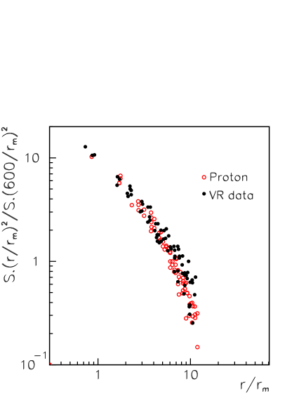
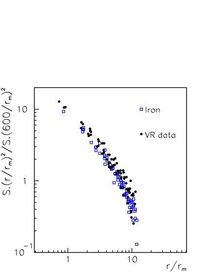
FIG. 3.: Comparison between lateral distribution measurements in a single event [24] and the simulated scintillator response in the configuration of VR array for $10^{19.1}$ eV proton and iron showers.

V Derivation of the primary mass composition

The nature of the primaries that initiate air showers is difficult to establish from the average properties of the data. For example, an average property can be explained with a mass composition of a single species (A) or by an appropriate mixture of species. However, with the Volcano Ranch array, accurate measurements of $\eta$ were made on a shower-by-shower basis for fixed bins of zenith angle separated by 80 g cm^-2  [21]. Thus the fluctuations of $\eta$ can be used to break this degeneracy. Linsley determined the precision of each measurement of $\eta$ and reported the average value of this quantity for each zenith angle bin.

The average error in $\eta$ from the fit made to the simulated lateral distributions ($\sigma_{sim}=0.029$), is smaller than the one reported by Linsley($\sigma=0.072$). To include within the simulation the effect of data reconstruction, we smeared each value of $\eta$ calculated by Monte Carlo using a Gaussian with a width chosen so that Linsley’s overall uncertainties in $\eta$ are reproduced i.e. $\sigma_{smear}=0.0662$ is found by quadrative subtraction of the average values of $\sigma_{sim}$ and $\sigma$.

This is a minor correction since the measurement accuracy is so much smaller than the intrinsic shower-to-shower spread (r.m.s.= 0.19). Thus, for each value of $\eta$ found from the Monte Carlo calculation, we have a corresponding and realistic estimate of its “experimental” uncertainty. We are thus able to make comparisons of Volcano Ranch data with our calculations.

As a further check, we have calculated the variation of $\eta$ with shower size and zenith angle with Monte Carlo and made comparisons with the Volcano Ranch data. The number of particles at ground level ($N_{fit}$) is obtained from a fit to the lateral distribution function (with $\alpha=1$) for fixed bins of zenith angle. The variation of $\eta$ with $N_{fit}$ from the calculation has been compared with the average functional form of $\eta$ given by Equation 3. The results of this comparison for $\sec\theta=$ 1.0 - 1.1 and 1.3 - 1.4 can be seen for proton and iron showers in Figure 4. The error bars indicate the r.m.s. spread of data which is very much greater than the r.m.s. spread of the mean. The shaded band represents the fit to Volcano Ranch data, including the errors given in Equation(3) for $a$ and $b$.

         

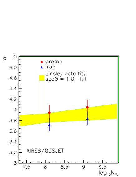
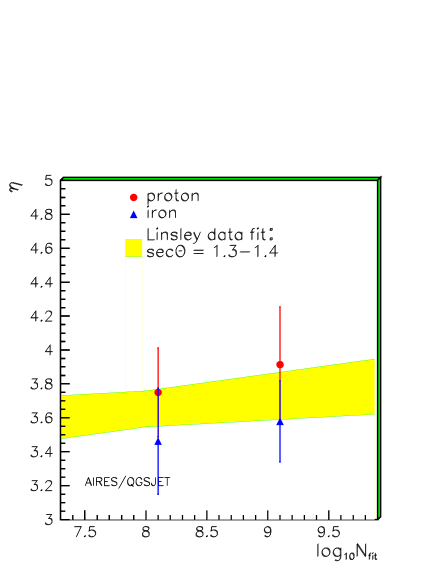
FIG. 4.: Comparison of $\eta$ as a function of shower size for $\sec\theta=1.0-1.1$ (left) and $\sec\theta=1.3-1.4$ (right) using aires/qgsjet98

The variation of $\eta$ with zenith angle is shown in Figure  5 for events with shower size in the range $\log N_{fit}=7.6-8.6$ (left) and $\log N_{fit}=8.6-9.6$ (right). One can see that the average form of $\eta$ over a realistic range of mass composition, from proton to iron, is well represented by the simulations. The error bars represent the r.m.s. spread as before.

         

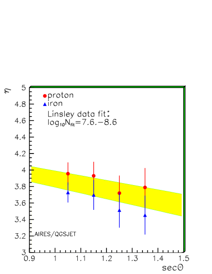
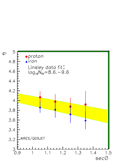
FIG. 5.: Comparison of $\eta$ as a function of $\sec\theta$ for the first bin (left) and second bin (right) in $logN_{fit}$

A Fitting VR data mass composition using finite Monte Carlo samples of different primaries.

We can estimate the primary mass that describes the Volcano Ranch data, assuming a bi-modal composition, using a maximum likelihood fit for the best linear combination of pure iron and pure proton samples to match the data sample. The available data are in bins of $\eta$ [23]: the number of data points in several bins is small, so a $\chi^{2}$ minimization is inappropriate. A maximum likelihood technique assuming Poisson statistics was adopted. The probability of observing a particular number of events $d_{i}$ in a particular bin is given by $\exp^{-f_{i}}\,f_{i}^{d_{i}}/d_{i}!$ where $f_{i}$ is the predicted value for the number of events in this particular bin. If we assume a bi-modal composition of proton and iron with fractions $P_{Fe}$ and $P_{p}$ then $f_{i}=C(P_{Fe}+P_{p})$ where $C$ is the overall normalization factor between numbers of data and Monte Carlo events. Estimates of the fractions $P_{j}$ are found by maximizing $\ln(L)=\Sigma d_{i}\ln(f_{i})-\ln(d_{i}!)-f_{i}$. Our Monte Carlo samples are at least ten times larger than the data sample to avoid effects of finite Monte Carlo data size.

         

FIG. 6.: The measured distributions of $\eta$ (data points) with histograms from Monte Carlo calculations of pure iron (left) and pure proton (right) with $1.0<\sec\theta<1.1$, using qgsjet98.

FIG. 7.: Composition fit from $\eta$ distribution for the first bin in $1.0<\sec\theta<1.1$, using qgsjet98. The points are the VR data and the solid line corresponds to the result of the fit.

In Figure 6 we compare the Monte Carlo results with the Volcano Ranch data points for near vertical showers. As can be seen the tail at large $\eta$ in the comparison with iron indicates that a lighter component is required to fit the experimental data. The best fit gives a mixture with (89 $\pm$ 5) % of iron, with a corresponding percentage of protons, and this distribution of $\eta$ is shown in Figure 7. One detail that Linsley did not describe is the distribution of shower sizes that comprise the data set. What is recorded is that the median energy was $10^{18}$ eV and that the shower sizes are between $4\times 10^{7}$ and $6\times 10^{9}$. This corresponds to an energy range approximately between $10^{17}$ eV and $10^{19}$ eV. To reproduce the data set, a differential energy spectrum of slope -3.5 was chosen for the primary energy spectrum. Simulations show that the whole area of the array was active above $10^{18}$ eV. Using this spectrum and the condition that the median energy be $10^{18}$ eV, the calculated threshold energy is approximately $10^{17.7}$ eV. Below $10^{18}$ eV the energy distribution of the data set was smoothed (always under the condition of median energy to be $10^{18}$ eV) assuming that the effective area of the detector increases with energy from the threshold up to $10^{18}$ eV. The conclusions about mass composition that we presently draw, are constrained by uncertainties in the details of the energy distribution of events recorded at VR. Additionally they are constrained by the hadronic model assumed.

The systematic error arising from our lack of knowledge of the energy distribution of the events has been estimated by repeating the fitting procedure with different energy spectra. From this analysis we estimate a systematic error of 12%. An additional source of systematic error is related to uncertainties in the hadronic interaction model: following the discussion in [1] which relates to the use of qgsjet98 rather than qgsjet01, the systematic shift in the fraction of iron is 14%. Showers that are calculated using qgsjet01 are found to develop higher in the atmosphere so that the fraction of Fe estimated is reduced from (89 $\pm$ 5)% to (75 $\pm$ 5)%.

         

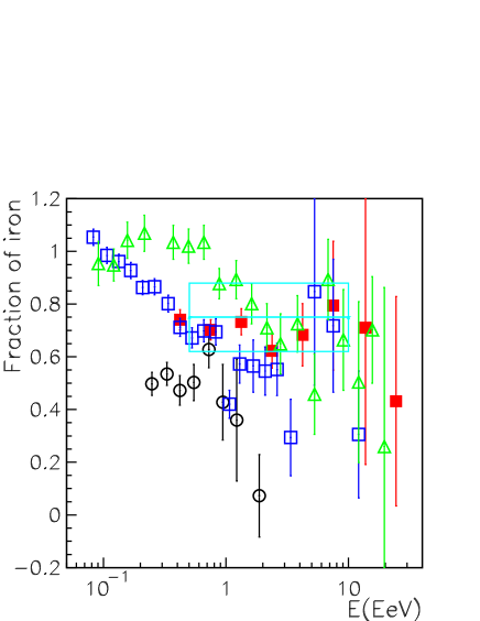
FIG. 8.: Fe fraction from various experiments: Fly’s Eye ($\triangle$), Agasa A100 ($\blacksquare$), Agasa A1 ($\square$) using sibyll 1.5 ([4] and references therein) and Haverah Park [1], using qgsjet98 ($\bullet$)(left) and qgsjet01 ($\circ$)(right). Mean composition determined in this paper with the corresponding error for the Volcano Ranch energy range using qgsjet98 (solid line rectangle at left) and an estimation of what it would result using qgsjet01 following [1] (dashed rectangle at right) is shown.

VI Comparison with other data

In Figure 8 we present the fraction of iron reported by Fly’s Eye, Agasa A100 and A1 (using sibyll as the hadronic model)  [6] and the results for Haverah Park [1] using qgsjet98 and qgsjet01. Also shown is the mean composition with the corresponding error we get for the Volcano Ranch energy range using qgsjet98 and an estimation of what we would get using qgsjet01 as it was done in Haverah Park [1].

The inconsistency that exists between several experiments which span different energy ranges, use different techniques is doubtless enhanced as different hadronic models are used for the interpretation of the raw data. The application of a consistent hadronic model [6] brings the results of AGASA into better agreement with the Fly’s Eye conclusion, while their original analysis stated that there is no indication of changing composition. In Figure 8 the iron fraction for Fly’s Eye and AGASA corresponds to the re-interpretation under the sibyll hadronic model, including triggering efficiency effects; the original analysis from AGASA is not presented here.

While Haverah Park, Volcano Ranch and Akeno-AGASA infer $X_{max}$, and hence the overall composition, from properties of secondary particle distribution at ground, Fly’s Eye and HiRes experiments observe a image of the longitudinal shower profile and derive $X_{max}$ directly. Nonetheless the estimates can be biased due to the poor knowledge of atmospheric properties as recent studies of atmospheric profiles have suggested  [28].

VII Conclusions

Measurements of the steepness of the lateral distribution $\eta$ were made at Volcano Ranch on a shower-to-shower basis for fixed bins of zenith angle. We have compared the measured distribution of $\eta$ to our Monte Carlo results for proton and iron primaries using qgsjet98 including the scintillator response of the detectors in the Volcano Ranch array. Our ability to reproduce Volcano Ranch lateral distribution measurements give us confidence that our analysis procedure is correct.

The cosmic ray mass composition, deduced from Volcano Ranch data, is compatible with mean fraction (89 $\pm$ 5(stat) $\pm$ 12(sys)) % of iron in a bi-modal proton and iron mix, in the whole energy range $10^{17.7}$ eV to $10^{19}$ eV, mean energy $10^{18}$ eV. Following the discussion in  [1], we estimate that this fraction would be reduced to 75 %, with the same qgsjet01 model adopted.

As mentioned above, some experiments find indications that the composition is becoming lighter with energy. However, in a recent work using Haverah Park data above $10^{19}$ eV, it was claimed that the observed time structure of the shower front can be best understood if iron primaries are dominant here  [27]. The differences between measurements on mass composition needs to be addressed further if more solid conclusions on the origin, acceleration or propagation of cosmic rays are to be reached. The rate of change with energy and the average mass are still under debate.