The VIRMOS deep imaging survey: III. ESO/WFI deep U-band imaging of the 0226-04 deep field.

In this paper we describe the $U-$band imaging of the F02 deep field, one of the fields in the VIRMOS Deep Imaging Survey. The observations were done at the ESO/MPG 2.2m telescope at La Silla (Chile) using the 8k $\times$ 8k Wide-Field Imager (WFI). The field is centered at $\alpha$(J2000)=02^h26^m00^s and $\delta$(J2000)=-04^∘30′00″, the total covered area is 0.9 $\deg^{2}$ and the limiting magnitude (50% completeness) is $U_{AB}\sim 25.4$ mag. Reduction steps, including astrometry, photometry and catalogue extraction, are first discussed. The achieved astrometric accuracy (RMS) is $\sim 0.2\arcsec$ with reference to the $I-$band catalog and $\sim 0.07\arcsec$ internally (estimated from overlapping sources in different exposures). The photometric accuracy including uncertainties from photometric calibration, is $<0.1$ mag. Various tests are then performed as a quality assessment of the data. They include: (i) the color distribution of stars and galaxies in the field, done together with the $BVRI$ data available from the VIMOS survey; (ii) the comparison with previous published results of $U-$band magnitude-number counts of galaxies.

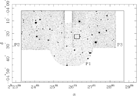
Figure 1: The VIRMOS F02 deep field. The images of the three pointings (P1, P2 and P3) are here combined for display purposes only: they have been treated separately in data reduction and catalog extraction. The full field is displayed in the upper plot. The outer solid–line rectangle shows the position of the $\sim 1.2\deg^{2}$ field taken in the $BVRI$ bands. Overlaid are the images of the three $U-$band pointings; masked areas at the borders of the images were removed. Note the circular shape of the P1 pointing, due to vignetting in the Loiano filter. The region in the inner box, where P1 and P3 overlap, is the one zoomed in the bottom plot: the accuracy of the astrometry can be seen from the absence of double sources.

1 Introduction

The VIMOS imaging survey (Paper I) represents the preparatory step of the deep redshift survey, which is now being carried out with the VIMOS spectrograph at the VLT UT3 at Paranal, Chile, by the VIMOS consortium. This preparatory multi-wavelength imaging survey has been done at the Canada-France Hawaii Telescope (CFHT) for the $BVRI$ bands (Le Fèvre et al. 2003, Paper I hereafter; McCracken et al. paperII (2003), Paper II hereafter), and at the ESO NTT telescope for the K imaging (Iovino et al. 2003, in prep). The near ultraviolet part of this survey was carried out at the ESO MPI 2.2m telescope with the WFI 8kx8k camera, in the framework of an approved ESO Large program (164.0-0089) scheduled since Period 63 in 1999, both in visitor and service mode.

The survey aims at covering $\sim 16\deg^{2}$ in $UBVRI$ with a 5 $\sigma$ limiting magnitude $I_{AB}\sim 24.5$, and a smaller $1.2\deg^{2}$ area reaching $I_{AB}\sim 25$, i.e. the VIMOS deep field. In the $U-$band, expected 5 $\sigma$ limiting magnitudes are $U_{AB}\sim 24$ mag for the wide survey, $U_{AB}\sim 26$ mag for the deep survey. In total the survey contains over $10^{6}$ galaxies in five colors and represents a major advance over other previous deep multicolor surveys, probing structures on scales of $\sim 20h^{-1}$ Mpc at $z\sim 1$.

Surveys in the radio continuum (Bondi et al. bondi (2003)) and with XMM (Pierre et al. pierre (2003)) were carried out on the deep field of the VIMOS imaging survey. The catalogs from the $U$ and $BVRI$ deep field are also foreseen to be used for the optical identification of the radio continuum survey (Ciliegi et al. in prep).

Until the availability of data from ground-based (e.g. the CFHLS and VST surveys) or space (e.g. the GALEX project) surveys, wide-field $U-$band data with medium depth and large sky coverage are not available yet. The $U-$band is essential to study the star formation properties of field galaxies in the nearby universe, and is also particularly suited to identify starburst galaxies, AGN, and QSO at moderate redshift. These aspects, as well the determination of the $U-$band luminosity function and the analysis of the morphological properties of galaxies compared to other bands, will be the subject of separate papers.

Compared to other existing $UBVRI$ surveys, the VIRMOS F02 deep field offers a good compromise between covered area and depth. The ESO imaging survey (EIS) in the Chandra Deep Field South (Arnouts et al. arnouts (2001)) is comparable in depth to our F02 deep field but covers a smaller area ($\sim 0.25\deg^{2}$). The Canada-France Deep Field survey (McCracken et al. cfdf (2001)) consists of four independent fields of $\sim 0.25\deg^{2}$ each, and the $U-$band limiting magnitude is $\sim$ 1 mag deeper than the VIRMOS deep field. The Combo-17 survey (Wolf et al. wolf (2003)) covers three fields with a total area $\sim 0.78\deg^{2}$ and is comparable in depth to the F02 deep field in the $U-$band. Deeper surveys (e.g. the William Herschel Deep Field, Metcalfe et al. metcalfe (2001) or more recently the FORS Deep Field, Heidt et al. heidt (2003)) were carried out on smaller areas ($\sim 7\times 7\rm{arcmin}^{2}$) only.

In this paper we will describe the observations, photometric calibration, catalogue extraction and validation for the deep field. The calibration steps are strongly related to those followed in the case of the overlapping deep $BVRI$ filters, which are described in Paper II. We refer to this paper for a detailed discussion of calibration issues when they are the same and emphasize those aspects that are peculiar to the $U-$band data.

The paper is organized as follows. In Section 2 we describe the observations for the deep pointings, the observing strategy and data reduction issues (pre-reduction, astrometric and photometric calibration). Catalog extraction is discussed in Section 3. Validation of the catalogs through a number of tests (comparison of stellar and galaxy colors with simulations, number counts) is done in Section 4. Conclusions are drawn in Section 5.

2 Observations and data reduction

2.1 Observations

The $U-$band deep pointing was observed during several observing runs since 1999 with the aim of covering $\sim 1\deg^{2}$ of the multiwavelength deep field planned within the VIMOS deep redshift survey. This deep field is centred at $\alpha$(J2000)=02^h26^m00^s and $\delta$(J2000)=-04^∘30′00″(see Fig. 1) and observations were carried out with the Wide-Field Imaging (WFI) mosaic camera mounted on the ESO MPI 2.2m telescope at La Silla, Chile. The camera was mounted at the Cassegrain focus of the telescope, giving a field of view of 34$\times$33 arcmin. It consists of a mosaic of 8 CCD detectors with narrow inter-chip gaps, yielding a filling factor of 95.9 % and a pixel size of $0.24\arcsec$. The WFI CCDs have a read-out noise of 4.5 e^- pix^-1 and a gain of 2.2 e^- ADU^-1.

The area covered for the $U$ deep field consists of three pointings partially overlapping (see Fig.1). When this survey started in 1999, a standard $U-$band Johnson filter was not available at the ESO MPI 2.2m telescope, so our team borrowed the one available at the Loiano observatory, and used this till a suitable $U-$band filter was acquired by ESO. One pointing was therefore imaged using the Loiano $U$ filter, which is a circular filter partially vignetting the field. Pointings 2 and 3 were imaged with the ESO U/360 filter.

The filter transmission curves are shown in Fig. 2; central wavelengths and FWHMs are given in Table 1, together with covered area and exposure times for each pointing. Note that, compared to the ESO filter, the Loiano filter is shifted to the red and also has a red leak at $\lambda\sim 7000$Å.

Figure 2: Transmission curves of the Loiano and ESO U/360 filters; curves before (dashed) and after (solid) the convolution with the CCD, telescope and atmosphere transmission are displayed. Note the red leak for the Loiano filter.

The efficiency during the observing campaign was hampered by bad weather conditions and a problem at the primary mirror support system which caused strong astigmatism on some images.

The exposure time for each individual frame was usually 2000s, and 1000s when astigmatism of the ESO MPI 2.2m telescope was severe. The total exposure time was 13.9 hrs for pointing P1, 20.3 hrs for pointing P2, and 17.8 hrs for pointing P3; see Table 1 for additional information on the observing log.

For each pointing, the sets of exposures were acquired in a dithered elongated-rhombi pattern. This sequence of dithered exposures ensures the removal of CCD gaps in the final coadded image, better flat fielding correction, efficient removal of bad pixel and columns and a more accurate astrometric solution in the final coadded image. The total area covered by the three pointings is $\sim 0.93\deg^{2}$. The effective area is actually smaller, $\sim 0.71\deg^{2}$, since: (a) a fraction of P1 is overlapping with P2 and P3; (b) the border regions of the images were masked when the noise was significantly higher due to either vignetting (P1) or the dithering steps; (c) a small fraction of the area in P2 and P3 is not covered in $BVRI$ and therefore was not taken into account when catalogs were built.

The atmospheric turbulence produced an average seeing of approximately $\rm{FWHM}\sim 1.3\arcsec$.

Pointing	Date	Filter	$\lambda_{c}$		FWHM		Area	Ditherings	Tot. exp	Seeing
			(Å)		(Å)		($\deg^{2}$)		(hr)	(arcsec)
1	Nov 99	Loiano	3620	3750	527	460	0.27	25x2000s	13.9	1.4
2	Oct 00, Nov 00	ESO U/360	3404	3540	732	536	0.30	22x1000s+ 25x2000s	20.3	1.3
3	Aug 01, Oct 01, Apr 02	ESO U/360	3404	3540	732	536	0.29	32x2000s	17.8	1.2

Table 1: Details concerning the pointings for the $U$ deep field. Filter central wavelengths and FWHM are given before and after (in italics) the convolution with the telescope, CCD and atmosphere transmissions. The area includes only the region where sources have been included in the catalog: it does not include border regions with vignetting or a low signal to noise ratio.

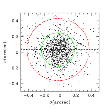
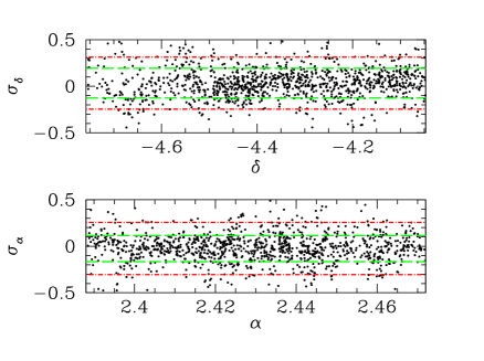
Figure 3: Astrometric residuals for unsaturated, point-like sources over the full field (P1, P2 and P3). Up: radial residuals; the inner and outer circles enclose 68% ($\sigma=0.21\arcsec$) and 90% ($\sigma=0.48\arcsec$) of the sources respectively; the cross shows the centroid, ($\sigma_{\alpha}$, $\sigma_{\delta}$)$=$(-0.02″, 0.03″). Bottom: residuals are displayed versus right ascension and declination; the lines display the residuals per coordinate (68%: $\sigma_{\alpha}=0.14\arcsec$, $\sigma_{\delta}=0.16\arcsec$; 90%: $\sigma_{\alpha}=\sigma_{\delta}=0.28\arcsec$).

2.2 Data reduction

Pre-reductions were carried out using the MSCRED package in IRAF. The CCD mosaic frames were bias and dark corrected, and flatfielded. Flatfield images were constructed combining a whole series of twilight sky images, taken during each observing night. Once the images were flatfielded, we noticed the presence of residual structures in the background sky, which should be treated in order to get a flat sky background in the final coadded images. A “super-flatfield” image was constructed from all the dataset for each pointing, using a 3-$\sigma$ rejection algorithm, for the removal of sources in the field. The procedures for astrometry, photometry and coaddition were approximately the same as those adopted in the analysis of $BVRI$ data. More details are given in Paper II; a short description follows where details peculiar to $U-$band data are emphasized.

2.2.1 Astrometry

Astrometry was performed using the astrometrix tool, which is part of the WIFIX package developed for the reduction of wide-field images. Astrometrix allows to compute an astrometric solution using both an external astrometric catalog and the constraint that the position of overlapping sources in different CCDs must be the same (global astrometry).

One of the main goals of this survey was to provide $U-$band fluxes of the sources detected in the $BVRI$ images. As described in more detail in Paper II, source detection for the $BVRI$ images was done as follows. A single $\chi^{2}$ image was first built from the $BVRI$ images, source detection was then done using SExtractor (Bertin & Arnouts bertin (1996)) in dual mode. This requires that source positions in all the images match at a subpixel level. Such level of accuracy was achieved as outlined in Paper II. The astrometric solution was first computed for the $I-$band image taking the USNO A-2 (Monet et al. 1998) as the astrometric reference catalog. A catalog of sources was then extracted from the resampled $I-$band image and used as reference catalog for the other bands ($UBVR$). During the astrometric procedure, the offset of $U-$band detected sources with respect to those matched in the $I-$band catalog was first computed for each CCD separately. This allowed to correct the displacement introduced by atmospheric refraction from the $I-$ to the $U-$ band. Finally, in the global astrometry step the astrometric solution was constrained for each CCD by both the positions from the $I-$band catalog and those from overlapping sources in all the other CCDs. Even if the three pointings were then resampled and coadded separately, in the global astrometry we used positions from all of them to increase the astrometric internal accuracy by using the position of the same source in the overlapping region of two different pointings (see Fig. 1).

To compute an accurate astrometry for $U-$band data is somewhat more difficult than for $BVRI$ data because of the smaller number of bright stars in the $U-$band. This implies that the astrometric solution may heavily rely on extended sources, for which the emission may peak at different positions in different bands. The achieved RMS astrometric accuracy, measured using $I-$band selected point-like sources only, is $<0.2\arcsec$ (see Fig. 3). The internal RMS, computed from overlapping sources in different exposures, is much smaller, $\sim 0.07\arcsec$.

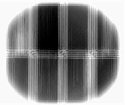
Figure 4: Weight map produced after coaddition of the P1 pointing.

2.2.2 Photometry

Photometric calibration was done taking several Landolt fields, so that we had at least one Landolt star in each CCD. Landolt fields were imaged also in $B$,$V$ to derive the filter color term, for each $U-$band filter used.

The calibration equation becomes:

$$U-u=\alpha(U-B)+\beta-\epsilon X,$$ (1)

Landolt fields were taken at different airmasses (X) during the night for all pointings with the exception of P2; (U-B) colors of the Landolt stars used in the calibration are in the range $0\leq(U-B)\leq 1.5$. This allowed us to compute the extinction coefficient $\varepsilon$: a value close to that expected for La Silla was obtained. For P2 this was not possible, so we took the average La Silla extinction coefficient for that period. Zero points, color terms and extinction coefficients computed for each pointing are given in Table 2. Recent photometric investigations (Manfroid, Selman & Jones manfroid (2001)) showed that the zero point changes across the WFI mosaic with a maximum difference of $\sim$ 0.08 mag as a consequence of non-uniform illumination and scattered light. As the Landolt fields are not wide enough to cover the whole WFI area and hence to compute one zero point for each CCD independently, the zero points we obtained represent an average over the whole mosaic from the different observed Landolt fields. The photometric accuracy in our data is therefore limited to $\sim 0.05$ mag, corresponding to about half the maximum difference in zero points over the entire WFI mosaic.

From the knowledge of the system transmission curves we then computed the AB corrections, that are displayed in the last column of Table 2.

Pointing	Date	Filter	$\alpha$	$\beta$	$\varepsilon$	RMS	X	AB corr
1	Nov 1999	Loiano	0.21$\pm$0.02	22.15 $\pm$ 0.06	0.43$\pm 0.02$	0.06	1.125	0.73
2	Nov 2000	ESO U/360	0.08$\pm$0.02	22.01 $\pm$ 0.02	0.49	0.06	1.105	0.94
3	Oct 2001	ESO U/360	0.08$\pm$0.02	22.10 $\pm$ 0.02	0.44$\pm$0.03	0.04	1.139	0.94

Table 2: Zero points, color terms and airmasses for the different pointings and filters. Date and airmass (X) refer to the image taken as reference when the relative photometry was computed. The last column gives the values to be added to the Vega-system magnitudes to obtain AB magnitudes.

To account for changes in airmass and atmospheric transparency, we used the Photometrix package in WIFIX. This package first applies the astrometric solution found for each CCD and then looks for overlapping sources in different CCDs. It then computes for each mosaic (defined as the set of 8 CCDs taken for each exposure) an additional term to the zero point ($z_{r,i}$) such that the average differences in fluxes of overlapping sources are minimized. An exposure taken in photometric conditions was chosen as reference, so that for it $z_{r,i}$=0: this image was taken in the same night as the Landolt fields used to make the photometry calibration. Since the P2 and P3 pointings are not connected, and P1 was taken with a different filter, we needed to run this step for each pointing separately.

2.2.3 Coaddition

After the astrometric solutions and flux scaling factors were computed, image coaddition was done using the SWarp tool developed by E. Bertin . SWarp allows to subtract the background, resample the images according to the astrometric solution, apply the flux scaling factor, and finally combine them. As in the case of the $BVRI$ images, resampling was done using a ”Lanczos-3” interpolation kernel, which corresponds to a sinc function multiplied by a windowing function. The coaddition was done computing the median of the images to optimize the rejection of spurious sources as cosmic rays or satellite tracks. As a consequence of the use of two different filters for the P1 and P2, P3 pointings, it was not possible to produce a single coadded image for the whole field. We therefore produced one image for each pointing; the size, pixel scale (0.205$\arcsec$ pix^-1) and orientation of each image was the same as that of $BVRI$ data so that catalogs can be extracted with the same $\chi^{2}$ technique (see Paper II). This allows to extract catalogs using SExtractor in dual mode, with the $\chi^{2}$ image as reference. In SWarp, each image may be associated to a weight-map to properly weight pixels during the coaddition step. This was particularly useful in the case of the Loiano filter, due to vignetting in the outer regions. Weight maps were first created using normalized flat fields; pixels flagged in the Bad Pixel Maps provided for WFI by ESO were then set to 0 in the weight map. For the pointing P1, we also set to 0 those pixels with a value $<0.6$ in the normalized flat field, thus allowing us to remove in the coaddition the regions affected by vignetting. Fig.4 shows the coadded weight map for P1.

Figure 5: Ratio of detected to input sources as a function of input magnitude: the input catalog consists of simulated point-like sources with a flat magnitude distribution. The dotted lines show the adopted 50% and 90% completeness magnitudes for each pointing. The histograms in the insets show the magnitude distribution of the spurious sources detected in the images with background only and no simulated sources.

3 Preparation of the catalogs

3.1 Photometric properties

A first estimate of the detection limiting magnitude for point-like sources was done on the background RMS map: this map was extracted for each pointing using SExtractor and the median background RMS ($\sigma$) was then computed. The limiting magnitude at 3$\sigma$ and 5$\sigma$ levels is mag$(n\sigma)=\beta-2.5\log(n\sigma\sqrt{A})$ where $n=3,5$, $A$ is the area of an aperture whose radius is the average FWHM of point-like sources, $\beta$ is the zero point (Eq. 1). We obtained $U_{AB}\sim$ 25.8 at 5$\sigma$ and $U_{AB}\sim$ 26.4 at 3$\sigma$.

Because of their definition, these values for the limiting magnitudes refer to the unrealistic case of objects with a flat radial surface brightness profile. A more accurate determination of the photometric limits of the survey was then done as follows. Catalogs were first extracted using SExtractor, where source detection was optimized using simulations of point-like sources. A background image was computed as outlined in Arnaboldi et al. (2002); a population of 2000 point-like objects with the same PSF of bright isolated stars in the field was added on this image, following a flat magnitude distribution (20.5 $\leq$ mag $\leq$ 27) and a random spatial distribution: the tasks in the ARTDATA package in IRAF were used. SExtractor was then run on that image and it was measured how many objects were detected and the faintest magnitude reached for a given detection threshold. The number of connected pixels required for source detection was set to 9 pixels: this gives a minimum signal to noise ratio of $\sim$ 3$\sigma$ for a detection threshold $\sim$ 1. The same process was repeated 20 times, giving a total of 40 000 sources and around 1500 sources per 0.25 magnitude bin. At the same time, we monitored the number of spurious sources, by matching the output catalogue from SExtractor with the input catalogue. The optimal threshold was the one that minimized the number of spurious detections with $U_{AB}<26$, without loosing input sources. Following these tests, we set the detection threshold to $\sim 0.7\sigma$ for the P1 pointing and $\sim 0.9\sigma$ for P2 and P3, over at least nine connected pixels.

Fig. 5 shows the results of the simulations (detected/input sources). In Table 3 we list the magnitude of completeness ($>$ 90% of the modeled objects in the input catalog are retrieved) and the limiting magnitude (50% of the modeled objects retrieved). The depth of P1 is comparable to that of P2 and P3 even if the exposure time is lower, since the Loiano filter is redder than the ESO filter and is thus somewhat more efficient, after convolution with the atmosphere. In order to check how many spurious detections should be expected at different magnitudes, we then run SExtractor on the background image before simulated sources were added. The result is displayed in the histograms in Fig. 5, which show that there are no spurious detections for magnitudes brighter than the 90% completeness magnitude; the peak occurs for magnitudes fainter than the detection limit ($U_{AB}\geq 26$) . Residual spurious detections for magnitudes close to the 50% limiting magnitude are later removed by the cross correlation with the catalog derived from the $\chi^{2}$ image.

Pointing		$m_{\rm comp}$	$m_{\rm lim}$	$\mu_{\rm comp}$	$\mu_{\rm lim}$
		(90%)	(50%)	(90%)	(50%)
1		25.0	25.5	25.7	26.2
2		24.9	25.3	25.8	26.3
3		24.9	25.3	25.7	26.2

Table 3: Completeness and limiting magnitudes and surface brightnesses (mag arcsec^-2) derived from simulated point-like and extended sources respectively. All values are in the AB system.

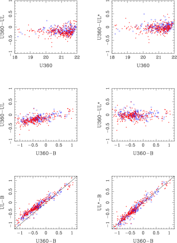
Figure 6: Difference in aperture magnitudes (5″diameter) of point-like and extended bright ($18<U<22$) sources taken with both the ESO (U360) and Loiano (UL) filters. $B-$band fluxes were taken from the VIRMOS catalog. The upper and middle panels show the differences in magnitudes before (left) and after (right) the color correction is applied (squares: P2; dots: P3). In the bottom panel $(U-B)$ colors from the Loiano and ESO filters are compared.

Similar simulations were done using extended sources, to compute the completeness and limiting surface brightness. Galaxies with De Vaucouleurs and exponential surface brightness laws were used as input sources to simulate elliptical and spiral galaxies respectively; total magnitudes of these sources were in the range $20<U_{AB}<26$. The same procedure as above was then followed, but this time we measured the peak surface brightness (defined as the surface brightness of the brightest pixel) of the simulated and detected sources. The so obtained values are also given in Table. 3.

3.2 Catalog extraction

In order to easily combine the catalogs derived from the $U$ and $BVRI$ images, it was decided to use the $BVRI$ $\chi^{2}$ image catalogue as reference for the extraction of sources in the $U-$band.

The $BVRI$ $\chi^{2}$ image catalogue is significantly deeper than the catalogue which can be derived using only the $U-$band image; the relative depths of the two catalogues can be judged by comparing the surface densities of objects, $\sim 10^{5}$ per square degree in the $\chi^{2}$ image catalogue (Paper II), and $\sim 10^{4}$ per square degree in the $U$ band catalogue. On the other hand, we would measure positive (spurious) flux in the background-subtracted $U$ frame at the position of sources detected in the $\chi^{2}$ image even if no significant $U$ source is detected (by definition a positive flux would be measured in about 50% random positions). To remove these spurious detections we adopted the following strategy. For each pointing (P1, P2 and P3), we extracted two catalogs:

• One catalog was extracted using SExtractor in the “dual image mode”, taking as input catalogue the one obtained from the $\chi^{2}$ image of the $BVRI$ dataset (see Paper II).

• One catalog was extracted in single-image mode, using a filtering Gaussian kernel and the detection threshold set as discussed above.

For both catalogs, Kron (magauto) magnitudes and aperture magnitudes at diameters of 15 pixels ($\sim 3\arcsec$) and 25 pixels ($\sim 5\arcsec$) were computed. As it concerns the required number of contiguous pixels, we used the same value that was adopted for the $BVRI$ images (see Paper II).

A cross-correlation was then done between coordinates of sources in the two catalogs; a maximum distance of $2\arcsec$ was adopted for matching. In addition, aperture magnitudes ($5\arcsec$ diameter) were also used as a further constraint in the cross-correlation: matching sources were rejected when the difference of $U-$band magnitudes obtained from the $\chi^{2}$ and single image catalogues was $>0.5$ mag.

After the cross correlation we computed the average difference between the magnitudes measured in the single and $\chi^{2}$ images: for all the three pointings we obtain $\langle\Delta U\rangle\leq 0.02$ mag with RMS values which change from $<0.05$ mag for bright sources ($U_{AB}<22$) to $\sim 0.1$ mag for fainter magnitudes. Considering (1) the different depths of the $U-$band and $\chi^{2}$ images and (2) the fact that for extended sources the peak of the emission may be different in the $U-$band compared to the $BVRI$ bands, we decided to keep in the final catalog the magnitudes measured on the single image rather than those computed using the parameters from the $\chi^{2}$ image.

As a consequence of the dithering strategy, regions close to the border of the image are covered by a small number of exposures: spurious sources are therefore produced either by a bad rejection of cosmic rays or by the high noise. We therefore removed from the catalogs all the sources located within a given distance from the border. $U-$band magnitudes were assigned to sources in the $\chi^{2}$ catalog only when they were detected in the single-image catalog with a magnitude brighter than the $3\sigma$ limiting magnitude, $U_{AB}=26.4$. For magnitudes brighter than the completeness limit, unmatched sources are mainly false detections (e.g. halos around bright stars) or sources not found in the $\chi^{2}$catalog (e.g. because of cosmetic defects). For fainter magnitudes, spurious detections due to correlated noise are more important in the single-image catalog (see Fig. 5) but are removed by the cross correlation with the $\chi^{2}$ catalog. The requirement on the magnitude helps to reject these spurious detections, removing $\leq$ 6% of sources for $U<25$ mag, $\sim$ 10% for fainter magnitudes.

The separation of extended vs. point-like sources was done on the $I-$band catalog, and is described in Paper II: such classification was done in the range $18<I_{AB}<21$, that is between the $I-$band saturation limit and the magnitude beyond which the separation between resolved and unresolved sources is less reliable. We verified on the half-light radius versus $U-$band magnitude plots that sources classified as point-like fall on the expected locus. The same plots were also used to estimate the average seeing in each pointing that is given in Table 1. In addition, bright nearby galaxies which are saturated in the $I-$band but not in the $U-$band were flagged as extended.

Finally, we computed for each filter the correction to bring the magnitudes to the AB system (see Table 2) and the Galactic extinction correction. The F02 field is characterized by a low interstellar extinction (see Paper I); according to the Schlegel et al. (schlegel (1998)) maps $0.023<E(B-V)<0.040$, with an average value $E(B-V)\sim 0.027\pm 0.002$ mag. This translates to an average correction for extinction $A_{U}\sim 0.14$ mag.

Figure 7: Comparison of colors for bright ( $U_{AB}<23.5$) point-like sources (dots) with: the library from Pickles (1998) (stars); the Kurucz model atmospheres (Kurucz kurucz (1979)) with $\log g=4.0$, [M/H]=0 (lower curve) and [M/H]=-5.0 (upper curve). Magnitudes in P1 were trasformed to the ESO filter photometric system.

Figure 8: Comparison of simulated and observed $(B-V)$ colors vs. $I$ magnitudes. Top: color-magnitude diagram. The upper panel shows the synthetic colors expected in the F02 area. The lower panel shows the observed colors for $U-$band selected ($U_{AB}<23.5$) point-like sources from the three pointings; the cuts at the faint and bright end are due to the fact that the selection of point-like vs. extended sources was done in the range $18<I_{AB}<21$ only. The solid line indicates the separation between halo and disk/thick disk stars. Bottom: The same as above, but plotted as a histogram.

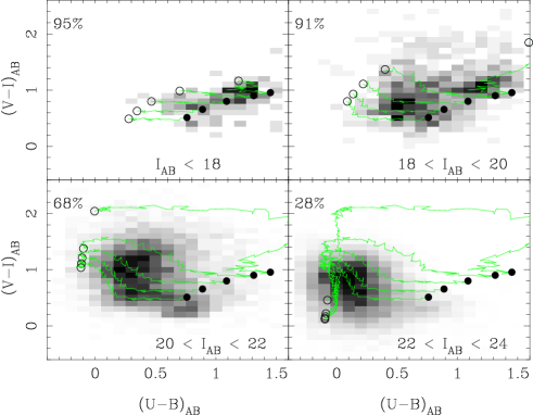
Figure 9: $(U-B)_{AB}$ vs. $(V-I)_{AB}$ colors for extended sources with $U_{AB}<25$. Colors are displayed as a grey-scale map where the level is proportional to the number of sources in a given color bin. Model tracks for early to late type galaxies are also displayed (starting from right to the left); the positions of lower and upper redshift are indicated by the filled and open circles respectively. Magnitudes in P1 were transformed to the ESO filter photometric system. The four panels show sources in different bins of $I_{AB}$, as follows. (a) $I_{AB}<18$, model tracks: $0.0<z<0.2$. (b) $18<I_{AB}<20$, model tracks: $0.0<z<0.4$. (c) $20<I_{AB}<22$, model tracks: $0.0<z<0.8$. (d) $22<I_{AB}<24$, model tracks: $0.0<z<1.5$. The value in the top left corner is the fraction of galaxies detected in the $U-$band with respect to those detected in the $I-$band, in each bin.

3.3 Color correction of the Loiano filter to the ESO filter

After catalogs were extracted, for each pointing we assessed the problem of bringing the $U-$band photometry to a single photometric system. We decided to convert the magnitudes measured in P1 with the Loiano filter to the ESO photometric system, since the latter is closer to the Johnson system. The advantage of doing so, rather than using Eq.1 to transform both magnitudes to the Johnson system and then computing the internal offset, is given by the fact that we can later use the ESO system transmission curve e.g. for comparison with model predictions.

As shown in Fig.1, the P2 and P3 fields taken with the ESO filter partially overlap with P1. For the overlapping sources, we therefore have photometry for both the $U-$band filters; in addition, $B-$band photometry is available from the CFHT data. We first extracted from the catalog bright ($20<U<22$) point-like sources; 35 and 46 sources were found for P2 vs. P1 and P3 vs. P1 respectively. From these we solved Eq.1 with no airmass ($\epsilon=0$), taking the ESO filter as reference (magnitudes not including the AB correction were used). Similar results were obtained for both P2 and P3: hence we merged the two sub-catalogs and finally obtained $\alpha=0.178$, $\beta=-0.08$ in Eq.1. The color term, as expected, is intermediate between the values found for the two filters from the calibration with standard stars (see Table 2). In Fig.6 we show the differences in magnitudes of both point-like and extended sources in the overlapping areas of the two filters before and after color correction. The average offset in magnitude after the correction is -0.01 mag (P1 vs. P2) and 0.04 mag (P1 vs. P3), with an RMS $\sim 0.1$. The same plot also provides an indirect check that photometry in P2 and P3 is consistent, as each of them is consistent with the P1 photometry in the overlapping areas.

The consistency with magnitudes obtained in the Johnson system by applying the color terms listed in Table 2 was checked as follows. Both the ESO and Loiano magnitudes were first transformed to the Johnson system. The same procedure as above was then followed to compute the offset between the Loiano and ESO photometry: we found $\alpha=0$ as expected and $\beta=-0.1$ mag. Loiano magnitudes were then transformed to the ESO system as discussed above, and then to the Johnson system. The agreement is within $\sim 0.08$ mag in the range $-2<(U-B)<2$.

4 Data quality assessment

In order to check the data quality of the $U-$band photometry, we performed a series of tests where we (i) compared colors of point-like and extended sources to those expected for stars and field galaxies; (ii) checked the number counts of galaxies and compared them with existing data in literature. In this analysis, magnitudes in the P1 pointing were first transformed to the ESO filter photometric system as described in Sec. 3.3; for those sources which were observed with both the Loiano and the ESO filter, the latter magnitude data were taken. In the final catalog, magnitudes are corrected for Galactic extinction.

4.1 Stellar colors

We first compared the colors of bright ($U_{AB}<23.5$) point-like sources with those obtained from the convolution of stellar templates (Pickles pickles (1998)) with the system transmission curves (filter + telescope + CCD + atmosphere). No correction for Galactic extinction is applied in this case. The result is displayed in Fig. 7: it can be seen that the agreement is good only for $(B-V)\geq$ 0.7. This is expected since for bluer colors the low-metallicity stellar population from the halo dominates over the disk population with solar metallicity. We therefore computed the colors produced using the Kurucz model atmospheres (Kurucz kurucz (1979)) with $\log g=4.0$ and [M/H]=0.0, -5.0 to reproduce solar and sub-solar metallicities (see also Lenz et al. Lenz (1998)). As displayed again in Fig. 7, the apparent excess in $(U-B)$ is in agreement with the colors produced by the low-metallicity model. The absence of observed stars at redder colors ($(U-B)>2.5$) is due to the cut in the $U-$band magnitudes, as it is explained later in more detail. Most of the sources outside the stellar locus with an ultraviolet excess ($(U-B)<0.6$) are likely to be quasars at $z<2.2$.

In order to verify whether the color distribution we obtained is consistent with that expected in our Galaxy, we show in Fig.8 (top) the synthetic color-magnitude (CM) diagram ($(B-V)$ vs. $I$) for a region of sky centered on P1 and a size of 0.9 $\deg^{2}$ (Degl’Innocenti & Cignoni, Private Communication). The code and recipes described in Castellani et al. (castellani (2002)) were used to this aim: the code provides $BVRI$ magnitudes for a Galactic stellar population model, including halo, disk and thick disk components.

We selected from the simulations those sources with $18<I_{AB}<21$ as this is the range where the point-like classification was done in our data. We expect to find only halo stars (i.e. metal poor objects) around $(B-V)\sim 0.5$, a mix of halo and thick disk stars in the interval $0.5<(B-V)<1.4$, and mainly disk stars (metal rich objects) around $(B-V)\sim 1.4$. Fig.7 shows that $(U-B)>2$ when $(B-V)>1$: therefore, when we compare simulated and observed color distributions we need to take into account the selection introduced by the cut in the $U-$band magnitude, $U_{AB}<23.5$. As the models do not provide $U-$band magnitudes, we proceed as follows. The limits $(U-B)>2$ and $U_{AB}<23.5$ imply that $B_{AB}<21.5$. From $(B-V)>1$ we obtain $V_{AB}<20.5$. Finally, Fig. 15 in Paper II shows that $(V-I)>1$ when $(B-V)>1$: we therefore obtain $I_{AB}<19.5$.

The same diagram is plotted in Fig.8 for the point-like sources in the VIRMOS deep field which were detected in the $U-$band. An exact match with the number of disk stars can not be expected as the selection due to the cut in the $U-$band was taken into account in an approximate way. The position of the two clumps centered at $(B-V)\sim 0.5$ and $(B-V)\sim 1.4$ is clearly visible (Fig 8, bottom). This confirms that the $(U-B)$ excess seen in Fig. 7 is due to the halo stars in the F02 field.

Figure 10: Galaxy magnitude-number counts from the VIRMOS $U-$band deep field compared with existing literature data. $U-$band magnitudes are in Vega system. The filled circles show the VIRMOS data (statistical error bars are displayed but are too small to be seen); magnitudes from P1 were transformed to the ESO filter photometric system. Literature data are taken from the N. Metcalfe’s collection. The dotted line shows the best fit computed in the range $18.5<U<22.5$. The dot-dashed lines show the 90% and 50% completeness limits. The histogram displays the number counts corrected for incompleteness (see text for details).

4.2 Field galaxy colors

$(U-B)_{AB}$ and $(V-I)_{AB}$ colors were compared with those obtained from model galactic spectra convolved with the system transmission curves. This was done using the make_catalog tool which is part of the HYPERZ package (Bolzonella et al. bolzonella (2000)): we used the built-in set of templates for early to late- type galaxies computed from the GISSEL98 spectral evolution library of Bruzual & Charlot (bruzual (1993)). As in Paper II, we divided our catalog of $U-$band detected extended sources in different bins of $I_{\rm AB}$ magnitude. Late-type galaxies are expected to increasingly dominate in the color distribution as we go to fainter magnitudes: early-type galaxies with faint $I$ magnitude are too faint to be included in the $U-$band catalog.

(i) $I_{AB}<18$. The brightest galaxies are clearly dominated by a low redshift population, $z<0.2$, of early to late-type galaxies (Fig. 9a).

(ii) $18<I_{AB}<20$. In Paper II it is shown that $(B-V)$ vs. $(V-I)$ colors for these galaxies are in agreement with those expected for a population of galaxies with $z$ = 0.0 - 0.5. The median redshift expected for this magnitude range is $z\sim 0.2$, according to spectroscopic surveys like the CFRS (Crampton et al. crampton (1995)). Consistent results are found looking at the $(U-B)$ vs. $(V-I)$ colors (Fig. 9b), where early to late type galaxies are all seen to contribute to the observed colors.

(iii) $20<I_{AB}<22$. The colors are well reproduced by a population dominated by late type galaxies with $z\sim$ 0.0 - 0.8, with a peak at $z\sim 0.35$ (Fig. 9c).

(iv) $22<I_{AB}<24$. The limiting magnitude $U_{AB}$ $\sim$25 implies that in this range we mainly select galaxies with bluer colors ($(U-B)_{AB}<0.2$): most of these are likely to be late type galaxies at $z<1$, with some contribution from higher redshift galaxies (Fig. 9d). Note that in this magnitude range less than 30% of the galaxies are detected in the $U-$band.

4.3 Number counts

The comparison of number counts of galaxies with literature data provides a good check for both the efficiency of the star-galaxy separation (done in the $I-$band in our case) and the quality of our photometry. For $U-$band data, this is complicated by the few published number counts and by the heterogeneity of the data (e.g. different photometric systems, no correction for galactic reddening). A collection of $U-$band number counts is provided in the Vega-system by N. Metcalfe’s (http://star-www.dur.ac.uk/$\sim$nm/, see also Metcalfe et al. metcalfe (2001)); we selected only those measurements from CCD observations. They are displayed in Fig.10. The offset among the different measurements is due to both the different $U-$band filters and the absence of reddening correction for some of the literature number counts. For example, in the case of Metcalfe’s WHDF data $E(B-V)_{WHDF}\sim 0.02$, so that after dereddening the WHDF number counts should be shifted by $\sim$ -0.1 mag (Heidt et al. heidt (2003)).

The $U-$band VIRMOS number counts were normalized to the area covered by the unmasked regions, taking into account the overlapping regions ($\sim 0.7\deg^{2}$). Number counts not corrected for incompleteness are displayed as filled circles in Fig.10. Our data are in very good agreement with those of Arnouts et al. (arnouts (2001)), which were also taken with ESO/WFI. A least-squares fit in the range $18.5<U<22.5$ gives a slope d(log N)/dm = 0.54$\pm$0.06. The histogram in Fig.10 shows the number counts corrected for the ratios of input to detected sources displayed in Fig. 5 (Sec. 3.1): after this correction, number counts are in agreement with the extrapolation from brighter magnitudes up to $U\sim 24.5$ ($U_{AB}\sim 25.5$).

5 Summary

$U-$band data obtained in the framework of the VIRMOS preparatory imaging survey for the F02 deep field were presented in this paper, as a complement to the $BVRI$ data presented in Paper II. Observations, data reduction and catalog extraction issues were first discussed. Various quality assessment tests were then performed. A good agreement is found between the observed stellar colors and those computed from the Kurucz model atmospheres; a component with sub-solar metallicity is required to fit the halo stellar population which dominates over the disk population for $(U-B)<1.5$. This is confirmed by the comparison with the color distribution of stars in our Galaxy based on the Castellani et al. (castellani (2002)) model. The colors of extended sources were compared with those obtained from template spectra of galaxies. These tests also allowed to check the photometric consistency of $U-$band and $BVRI$ data. Number counts for extended sources were finally computed and compared with other $U-$band data in literature.

- (1) Arnaboldi, M., Aguerri, J. A. L., Napolitano, N., et al., 2002, AJ, 123, 760
- (2) Arnouts, S., Vandame, B., Benoist, C., et al., 2001, A&A, 379, 740
- (3) Bertin, E.& Arnouts, S., 1996, A&AS, 117, 393
- (4) Bolzonella, M. , Miralles, J.M., Pelló, R. , 2000, A&A, 363, 476
- (5) Bondi, M., Ciliegi, P., Zamorani, G., et al., 2003, A&A, 403, 857
- (6) Bruzual, G., Charlot, S., 1993, ApJ 405, 538
- (7) Castellani, V., Cignoni, M., Degl’Innocenti, S., et al., 2002, MNRAS, 334, 69
- (8) Crampton, D., Le Fevre, O., Lilly, S.J., and Hammer, F., 1995, ApJ, 455, 96
- (9) Ellis, R.S., Colless, M.M., Broadhurst, T.J., et al., 1996, MNRAS, 280, 235
- (10) Guhathakurta, P., Tyson, J.A., and Majewski, S.R., 1990, in Evolution of the universe of galaxies, ASP, 304
- (11) Heidt, J., Appenzeller, I., Gabasch, A., et al., 2003, A&A, 398, 49
- (12) Hogg, D.W., Pahre, M.A., McCarthy, J.K., et al., 1997, MNRAS, 288, 404
- (13) Kochanek, C.S., Pahre, M.A., Falco, E., et al., 2001, ApJ, 560, 566
- (14) Kurucz, R.L. 1979, ApJS, 40, 1
- (15) Le Fèvre, O., Mellier, Y., McCracken, H.J., et al., 2003, astro-ph/0306252 , submitted to A&A (Paper I)
- (16) Lenz, D.D., Newberg, H.J., Rosner, R., et al., 1998, ApJS, 119, 121
- (17) McCracken, H.J., Le Fèvre, O., Brodwin, M., et al., 2001, A&A, 376, 756
- (18) McCracken, H.J., Radovich, M., Bertin, E., et al., 2003, A&A, 410, 17 (Paper II)
- (19) Manfroid, J., Selman, F., and Jones, H., 2001, The Messenger, 104, 16
- (20) Metcalfe, N., Shanks, T., Campos, A., et al., 2001, MNRAS, 323, 795
- (21) Monet, D., Bird, A., Canzian, B., et al., 1998, U.S. Naval Observatory Flagstaff Station (USNOFS) and Universities Space Research Association (USRA) stationed at USNOFS
- (22) Pickles, A.J., 1998, PASP, 110, 863
- (23) Pierre, M., Valtchanov, I., Santos, S. Dos, et al., 2003, astro-ph/035192
- (24) Schlegel, D., Finkbeiner, D.P., and Davis M., 1998, ApJ, 500, 525
- (25) Songaila, A., Cowie, L.L., and Lilly, S.J., 1990, ApJ, 348, 371
- (26) Wolf, C., Meisenheimer, K., Rix, H.-W., et al. 2003, A&A, 401, 73