Large-Scale Structure Shocks at Low and High Redshifts

Abstract

Cosmological simulations show that, at the present time, a substantial fraction of the gas in the intergalactic medium (IGM) has been shock-heated to $T\gtrsim 10^{5}\mbox{ K}$. Here we develop an analytic model to describe the fraction of shocked, moderately overdense gas in the IGM. The model is an extension of the Press & Schechter (1974) description for the mass function of halos: we assume that large-scale structure shocks occur at a fixed overdensity during nonlinear collapse. This in turn allows us to compute the fraction of gas at a given redshift that has been shock-heated to a specified temperature. We show that, if strong shocks occur at turnaround, our model provides a reasonable description of the temperature distribution seen in cosmological simulations at $z\sim 0$, although it does overestimate the importance of weak shocks. We then apply our model to shocks at high redshifts. We show that, before reionization, the thermal energy of the IGM is dominated by large-scale structure shocks (rather than virialized objects). These shocks can have a variety of effects, including stripping $\lesssim 10\%$ of the gas from dark matter minihalos, accelerating cosmic rays, and creating a diffuse radiation background from inverse Compton and cooling radiation. This radiation background develops before the first stars form and could have measurable effects on molecular hydrogen formation and the spin temperature of the 21 cm transition of neutral hydrogen. Finally, we show that shock-heating will also be directly detectable by redshifted 21 cm measurements of the neutral IGM in the young universe.

1. Introduction

One of the major achievements of cosmology over the past two decades has been the development of a coherent and testable paradigm for structure formation. In the modern picture, small density inhomogeneities imprinted on the universe during inflation grow continuously through gravitational instability. These density fluctuations still have small amplitude at the time of cosmological recombination ($z\sim 1000$), when the cosmic microwave background (CMB) is last scattered. At this epoch, structure formation is straightforward to study analytically because the fluctuations are still linear. Observations of the CMB have shown convincing evidence that our theories of structure formation accurately describe the universe at this early phase (e.g., Spergel et al. 2003). Eventually, the perturbation amplitude grows sufficiently large for nonlinear effects to become important: at this point the first gravitationally bound structures begin to form. The structure formation problem then passes beyond the scope of analytic approaches (except in the case of perfectly spherical collapse; Gunn & Gott 1972). The most successful approximation for studying the properties of gravitational instability in the nonlinear regime is the so-called Zel’dovich approximation (Zel’Dovich, 1970), which uses Lagrangian (rather than Eulerian) perturbation theory. The theory shows that collapse will occur first along a single axis, creating a “pancake” or sheet, then along a second axis, creating a filament, before finally converging towards a single point.

Fully non-linear treatments of structure formation had to await the development of numerical simulations. These simulations confirm the behavior predicted by the Zel’dovich approximation: at low redshifts, the matter in the universe organizes itself into a complex network of sheets and filaments (with galaxies and galaxy clusters at their intersections) known as the “cosmic web.” This paradigm has had admirable success reproducing the large-scale distribution of galaxies in redshift surveys (e.g., de Lapparent et al. 1986) and in describing the absorption features of the Ly$\alpha$ forest (e.g., Cen et al. 1994; Hernquist et al. 1996; Theuns et al. 1998).

While the dark matter accretes smoothly onto the cosmic web, the baryons do not: their infall velocities onto these structures often exceed the local sound speed and a complex network of shocks forms. Probably most important are the well-known virial shocks that form when halos collapse. However, cosmological simulations also contain many shocks outside of collapsed halos; these fill a fair fraction ($\sim 10\%$) of the volume of the universe (Cen & Ostriker, 1999; Keshet et al., 2003; Ryu et al., 2003) and play an important role in shaping the properties of baryons in the local universe. Simulations predict that $\gtrsim 20\%$ of all baryons are in the “warm-hot intergalactic medium” (WHIM) with $T\sim 10^{5}$–$10^{7}\mbox{ K}$ (Davé et al., 2001), most of which have densities below those characteristic of virialized objects.

Unfortunately, there is little analytic understanding of the distribution of shocks in the intergalactic medium (IGM). Cen & Ostriker (1999) argued that the characteristic temperature of the gas can be computed by simply associating the postshock temperature with a fluctuation collapsing over the age of the universe that has just become nonlinear at the present epoch. This provides a rough guide to the expected strength of the shocks but does not predict how much gas has been shocked or give a detailed temperature distribution. Nath & Trentham (1997) expanded this treatment using the Zel’dovich approximation to give rough estimates of the fraction of gas in the WHIM phase, but they were not able to predict the detailed properties of shocks at any redshift.

There has also been little consideration of the role that similar large-scale structure shocks play at higher redshifts. One reason that they are significant in the local universe is that the characteristic shock temperature ($T_{\rm sh}\sim 10^{7}\mbox{ K}$; see Davé et al. 2001) is much larger than the mean temperature of the photoionized IGM ($T_{\rm IGM}\sim 10^{4}\mbox{ K}$). As redshift increases, $T_{\rm sh}$ decreases rapidly; at $z\gtrsim 2$, the characteristic temperature given by Cen & Ostriker (1999) is not much larger than $T_{\rm IGM}$, so we expect strong shocks to be much less common. However, before reionization, the typical temperature of the IGM is much smaller and shocks can again become important (despite the much smaller-scale perturbations that collapse). Because shocks occur in overdense regions, where galaxies also preferentially occur, they obviously help to determine the environments in which most galaxies reside. The large-scale environment has important consequences for feedback from (and on) collapsed objects, but this point has not been considered in the past.

In this paper, we consider a new analytic model for the temperature distribution of shocked, moderately overdense gas in the IGM. We are guided by the fact that the distribution of collapsed objects is well-described, to a surprisingly high precision, by the Press-Schechter formalism (Press & Schechter, 1974). The key ingredients to this model are (1) Gaussian statistics for the density field and (2) spherical collapse of perturbations in the nonlinear regime. Motivated by the success of this formalism, we use the same assumptions to model shocked gas in the IGM. We show that our simple model provides a reasonable fit to existing (low-redshift) simulation data if only strong shocks are considered. In §2, we present our formalism for the large-scale structure shocks and use it to describe the basic properties of shocks at both low and high redshifts. We then move on to consider the role that high-redshift shocks might play. In §3 we describe three important effects that the shocks can have: accelerating particles to high energies, creating a diffuse background radiation field (principally through cooling radiation), and stripping minihalo gas. In §4 we consider the observable consequences of high-redshift shocks. Finally, we summarize our main conclusions in §5.

Throughout the discussion we assume a flat, $\Lambda$–dominated cosmology, with density parameters $\Omega_{m}=0.3$, $\Omega_{\Lambda}=0.7$, and $\Omega_{b}=0.047$ in matter, cosmological constant, and baryons, respectively. In the numerical calculations, we assume $h=0.7$, where the Hubble constant is $H_{0}=100h\mbox{ km s${}^{-1}$ Mpc${}^{-1}$}$. We take a scale-invariant primordial power spectrum ($n=1$) normalized to an amplitude of $\sigma_{8}=0.9$ on 8$h^{-1}$ Mpc spheres. These values are consistent with the most recent measurements (Spergel et al., 2003).

2. A Model of Shocks from Large-Scale Structure

Following Cen & Ostriker (1999) and Keshet et al. (2003), we associate large-scale shocks with the collapse of nonlinear objects. The shock velocity $v_{s}$ is then approximately equal to the length scale of the perturbation divided by the age of the universe, or

$$v_{s}\approx H(z)R_{p},$$ (1)

where $R_{p}$ is the physical radius that the region would have had if it expanded uniformly with the Hubble flow (i.e., $4\pi R_{p}^{3}/3=M_{s}/\bar{\rho}_{z}$, where $M_{s}$ is the mass of the shocked region and $\bar{\rho}_{z}$ is the mean density of the universe at redshift $z$). The postshock temperature $T_{\rm sh}$ is then

$$T_{\rm sh}=\eta\frac{\mu m_{p}}{\gamma k_{B}}\,v_{s}^{2},$$ (2)

where $\mu m_{p}$ is the mean particle mass, $\gamma$ is the adiabatic index of the gas, and $\eta$ is the square of the Mach number of the shock in the downstream medium. Given a shock velocity and the sound speed of the IGM gas, $\eta$ is fixed in terms of $\gamma$ by the jump conditions; however, the definition of the shock velocity in equation (1) is only approximate, and we let $\eta$ encapsulate uncertainties in both the collapse time and the relevant length scale. In most of the following discussion we will assume strong shocks, for which $\eta=5/16$ (if $\gamma=5/3$). Note that the shock temperature depends on both the mass of the perturbation and on redshift. Cen & Ostriker (1999) and Davé et al. (2001) argued that choosing $R_{p}$ to be the length scale associated with the characteristic nonlinear mass at a given epoch reproduces the typical temperature of the WHIM gas in their simulations.

In order to compute the distribution of shocks, we make an analogy with the usual Press-Schechter mass function (Press & Schechter, 1974). The fundamental assumptions behind this mass function are: (i) the initial density field is Gaussian, and (ii) the threshold overdensity for a particle to be attached to a halo is given by the dynamics of a collapsing spherical top-hat perturbation. In this model, the fraction of mass in collapsed halos of mass $M>M_{0}$ is

$$F(M>M_{0},z)={\rm erfc}\left[\frac{\delta_{c}(z)}{\sqrt{2}\sigma(M_{0})}\right].$$ (3)

Here $\sigma(M_{0})$ is the variance in the density power spectrum smoothed over a mass scale $M_{0}$ and $\delta_{c}(z)=\delta_{c0}/D(z)$ is the linearly extrapolated overdensity corresponding to the collapse of a spherical perturbation. $D(z)$ is the cosmological growth factor and $\delta_{c0}\approx 1.69$ depends very weakly on the assumed cosmology. The mass function can be obtained by simply differentiating equation (3). This mass function matches the distribution measured in cosmological simulations to good accuracy, although modifications including ellipsoidal (rather than spherical) collapse do improve the fit somewhat (Sheth & Tormen, 1999; Jenkins et al., 2001), though perhaps not at the highest redshifts (Jang-Condell & Hernquist, 2001).

Here we make the ansatz that we can identify shocks with a different density threshold $\delta_{x}$ during the collapse. The entire Press-Schechter formalism carries over to our situation so long as we change the density threshold from that for collapse to the new value and choose the smoothing scale $M_{\rm sh}$ for a specified shock temperature $T_{\rm sh}$ through equations (1) and (2). The resulting temperature distribution is

$$\left[\frac{df}{dT_{\rm sh}}\right]_{\rm naive} = \frac{3}{\sqrt{2\pi}}\,\frac{M_{\rm sh}}{T_{\rm sh}}\,\left|\frac{d\ln\sigma}{dM}\right|_{M_{\rm sh}}$$ (4)

$$\times\frac{\delta_{x}(z)}{\sigma(M_{\rm sh},z)}\,\exp\left[\frac{\delta_{x}^{2}(z)}{2\sigma^{2}(M_{\rm sh},z)}\right],$$

where $df$ is the fraction of IGM gas (by mass) that is shocked to a temperature in the range $(T_{\rm sh},T_{\rm sh}+dT_{\rm sh})$. For reference,

$$M_{\rm sh} = 10^{13}\mbox{ M${}_{\odot}$}\left(\frac{\gamma}{5/3}\,\frac{0.6}{\mu}\,\frac{5/16}{\eta}\,\frac{T_{\rm sh}}{10^{6}\mbox{ K}}\right)^{3/2}$$ (5)

$$\times\left[\frac{1+z}{h(z)}\right]^{3}\left(\frac{\Omega_{m}}{0.3}\right),$$

where $h(z)=[\Omega_{m}(1+z)^{3}+\Omega_{\Lambda}]^{1/2}$. Because the $T_{\rm sh}$–$M_{\rm sh}$ relation is itself redshift-dependent, the redshift dependence of $\sigma$ cannot be factored out (unlike for the mass function). Also, we are interested only in the fraction of gas at a given temperature, not in the number density of such objects (which would be more sensitive to the non-spherical nature of collapse). In all other respects equation (4) is analogous to mass function calculations.

We note that both $\eta$ and $\delta_{x}$ are essentially free parameters in our formalism: in the purely spherical model, shocks do not actually appear until complete collapse, so the density threshold and shock velocity are ad hoc additions to the model. However, we will show below (see §2.1) that a simple, physically motivated set of choices provides a reasonable description of the existing simulation data for strongly shocked material. A plausible point for the shock to first appear is turnaround [$\delta_{x}\approx 1.06/D(z)$], the point at which the perturbation breaks off from the cosmological expansion. In purely spherical collapse, of course, no shocks would appear until shell-crossing occurs at virialization. However, turnaround marks the point at which the flow begins to converge. It is therefore reasonable to expect asymmetries in the collapse to begin to shock the gas at this point. Another advantage of associating shocks with turnaround is that the shock velocity in equation (1) exactly equals the peculiar velocity of the collapsing gas. Because most shocks are strong, we then assume $\eta=5/16$ for simplicity. We expect this choice to work best for regions with infall velocities much larger than the IGM sound speed. If the two are comparable, asymmetries in the collapse would have to be extremely strong for shocks to develop before shell-crossing. In this regime, we might therefore expect $\delta_{x}$ to be closer to $\delta_{c}$.

We also note that our formalism does not describe (or replace) virial shocks around collapsing halos. The “large-scale structure shocks” that we describe have much lower velocities because they occur earlier in the infall process. If we compare the shock temperature $T_{\rm sh}$ on a given mass scale to the virial temperature $T_{\rm vir}$ on the same scale, we find

$$\frac{T_{\rm vir}}{T_{\rm sh}}\simeq 4\frac{(1+z)^{3}}{h^{2}(z)}\left(\frac{\gamma}{5/3}\,\frac{5/16}{\eta}\right)\left(\frac{\Omega_{m}}{0.3}\right)^{2/3}\left[\frac{\Omega_{m}}{\Omega_{m}(z)}\right]^{1/3},$$ (6)

so the virial shocks will still be relatively strong.

There is one more subtlety in computing the temperature distribution: a particular trajectory that reaches $\delta_{x}(z)$ at some mass $M_{\rm sh}$ may reach $\delta_{c}(z)$ at another mass $M_{h}<M_{\rm sh}$. Physically, the particle could belong to a galaxy embedded inside a large-scale filament or sheet. We wish to exclude such gas from our distribution because it does not truly belong to the IGM. (It will also be at a different temperature: the gas initially virializes and then cools.) Fortunately, it is straightforward to identify these particles in the Press-Schechter model. Given that a particle has $(\delta_{x},M_{\rm sh})$, we wish to compute the probability that it has $(\delta_{c},M_{h})$. The problem is formally identical to the “progenitor” problem solved by Lacey & Cole (1993), with the solution

$$\frac{dp}{dM_{h}} = \sqrt{\frac{2}{\pi}}\frac{\sigma(M_{h})[\delta_{c}(z)-\delta_{x}(z)]}{[\sigma^{2}(M_{h})-\sigma^{2}(M_{\rm sh},z)]^{3/2}}$$ (7)

$$\times\left|\frac{d\sigma}{dM}\right|_{M_{h}}\exp\left\{\frac{-[\delta_{c}(z)-\delta_{x}(z)]^{2}}{2[\sigma^{2}(M_{h})-\sigma^{2}(M_{\rm sh},z)]}\right\}.$$

Here $dp/dM_{h}$ is the probability that a particle is contained in a halo of mass $M_{h}$ at $z$, given that it is part of a shock with mass scale $M_{\rm sh}$ at $z$. Then

$$\frac{df}{dT_{\rm sh}}=\left[\frac{df}{dT_{\rm sh}}\right]_{\rm naive}\left[1-\int_{M_{\rm min}}^{M_{\rm sh}}dM_{h}\frac{dp}{dM_{h}}\right].$$ (8)

We note that this prescription fits nicely into the “merger tree” algorithm commonly used in “extended Press-Schechter” studies (e.g., Lacey & Cole 1993). To compute the probability that a halo of mass $M_{h}$ will merge into a halo of mass $M_{\rm sh}$ at a later time $z_{v}$, we simply substitute $\delta_{x}(z)\rightarrow\delta_{c}(z_{v})$ in equation (7). Clearly, $z_{v}$ is fixed by the dynamics of collapse, $D(z_{v})=(\delta_{x}/\delta_{c})D(z)$. But this is the same relation as between the collapse and turnaround times in the spherical collapse model. We therefore find that the probability for a halo to lie in a turnaround shock of a region with mass $M_{\rm sh}$ at $z$ is the same as for the halo to lie in that region once it has collapsed.

The correction for bound objects would not be needed if the large-scale shocks were able to strip gas from collapsed objects. In the local universe, this occurs through ram pressure stripping and is fairly inefficient: in galaxy clusters, observations and simulations show that the timescale is short only in dense cluster cores (Quilis et al., 2000), and it is likely to be much longer in the low-density IGM. However, if the gas in a bound object is unable to cool radiatively and is then shocked during infall, it may be able to escape its host halo into the IGM. We will examine the implications of this process in detail in §3.3.

Note that the postshock temperature depends on the whether the gas is ionized or neutral. Any shock with $T_{\rm sh}>10^{4}\mbox{ K}$ will ionize gas after the shock, decreasing the actual temperature of the postshock gas by a factor $\sim 2$. If the gas is originally neutral, the shock will also lose energy ionizing the gas. For simplicity, we assume that the universe is completely ionized for all redshifts lower than the reionization redshift, $z<z_{r}$, and neutral for $z>z_{r}$. The temperatures we quote for shocks before reionization do not include ionization by the shock; they should thus be interpreted as the mean thermal energy per baryon. The reionization redshift also affects the minimum halo mass able to colllapse. If the universe is neutral and cold, we take the “filter mass” $M_{\rm fil}$ or time-averaged Jeans mass, as the minimum collapse mass (Gnedin & Hui, 1998). (Because turnaround shocks occur earlier in collapse than virialization does, we actually evaluate $M_{\rm fil}$ at the redshift corresponding to collapse of the object.) If the universe is ionized, we take the minimum mass to have $T_{\rm vir}>2\times 10^{5}\mbox{ K}$, below which gas infall is suppressed by photoionization heating (Efstathiou, 1992; Thoul & Weinberg, 1995; Navarro & Steinmetz, 1997), although near the time of reionization this probably overestimates the minimum mass (Dijkstra et al., 2003).

2.1. Comparison to Simulations

While we have presented a plausible picture in which $\eta$ and $\delta_{x}$ are chosen to match strong shocks at halo turnaround, these are actually free parameters that are not fixed by our model. In Figure 1, we show how their choice changes our differential temperature distribution function, $df/dT$. The top panel shows $\eta=0.16,\,0.24$, and $5/16$ (dotted, short-dashed, and solid curves, respectively), with $\delta_{x}=1.06$. [Note that the simulations of Keshet et al. (2003) suggest $\eta\approx 0.16$.] The sharp rise at low temperatures is the effect of the finite Jeans mass that we have imposed. Structures collapsing near the mass threshold cannot have any gaseous subcomponents, so the fraction of gas associated with bound objects rapidly approaches zero. The effect of varying $\eta$ is simply to translate the distribution along the temperature axis: we have not changed the fraction of mass associated with each mass scale, only the temperature associated with that scale. The bottom panel fixes $\eta=5/16$ but sets $\delta_{x}=0.8,\,1.06$, and $1.20$ (long-dashed, solid, and dash-dotted curves, respectively). The effect here is more subtle: for example, by increasing the threshold overdensity required for shocks, we decrease the mass fraction at each temperature. Because $\sigma(M)$ is not linear, the characteristic temperature also changes (i.e., the peak of the temperature distribution).

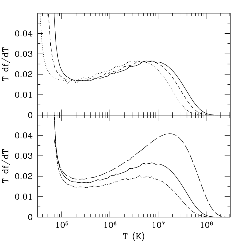
Figure 1.— The distribution of gas temperature at $z=0$, not including collapsed objects. Top panel: The curves have $\eta=0.16,\,0.24$, and $5/16$ (dotted, short-dashed, and solid lines, respectively); all assume $\delta_{x}=1.06$. Bottom panel: The curves have $\delta_{x}=0.8,\,1.06$, and $1.2$ (long-dashed, solid, and dot-dashed lines, respectively); all assume $\eta=5/16$.

Comparison to Figure 5 in Davé et al. (2001) shows that our fiducial choice gives a reasonably good fit to the shape of the temperature distribution at $z=0$. We find that $\sim 13\%$ of the gas is shocked to high temperature, compared to $\sim 25\%$ in the simulations. The comparison is somewhat difficult because Davé et al. (2001) include both bound objects (in particular galaxy groups) and gas at or near the mean density that is nevertheless shocked to high temperatures (see their Figure 4), while we expect our formalism to describe only the moderately overdense gas. We also find that our formalism overestimates the fraction of gas with $T_{\rm sh}\sim 10^{5}\mbox{ K}$. This is not surprising, because these shocks correspond to systems fairly close to the minimum mass for galaxy formation in an ionized medium. The infall velocities are therefore not much larger than the sound speed of the gas, and shocks probably develop only later in the collapse process for such objects. We expect our model to apply best when the characteristic shock speed is much larger than the sound speed of the IGM. On the other hand, capturing weak shocks is difficult in simulations with finite resolution (Keshet et al., 2003; Ryu et al., 2003), and they may underestimate the fraction of gas shocked to moderate temperatures.

2.2. Temperature Evolution of the IGM

We can now compute the temperature evolution of the IGM, including shocks at both turnaround and virialization. The results are shown in Figure 2. We assume that the universe is reionized at $z_{r}=8$; at this point the minimum mass for collapse increases substantially. The top panel shows the fraction of gas that is part of the shocked phase, $F_{\rm sh}$, at a given redshift (solid curve) as well as the fraction that is part of collapsed objects (dashed curve). The upper and lower dotted curves show $F_{\rm sh}$ before reionization if we only include shocks with $T_{\rm sh}>10^{4}\mbox{ K}$ and $10^{5}\mbox{ K}$, respectively. The bottom panel shows the mass-averaged temperature of the IGM. The solid line is for shocked gas while the dashed line is for collapsed gas (the temperature of each halo is set to $T_{\rm vir}$, and we have used the Press-Schechter mass function for the number density of halos at each mass). The dotted line shows the mean temperature from shocks if we include only those with $T_{\rm sh}>10^{4}\mbox{ K}$ (i.e., ionizing shocks). We set the temperature of the rest of the gas to zero in each case. The thermal energy of the IGM is dominated by shocked gas at $z\gtrsim 5$. At the present time, however, virialized objects determine the mean temperature: so long as a fair fraction of the mass is in such objects, their strong bounding shocks dominate over the IGM shocks [compare to equation (6)].

Figure 2.— Top panel: The fraction of gas in the shocked phase (solid curve) and in collapsed objects (long-dashed curve). The upper and lower dotted curves show the fraction with $T_{\rm sh}>10^{4}\mbox{ K}$ and $10^{5}\mbox{ K}$, respectively. We have assumed that reionization occurs instantaneously at $z_{r}=8$, at which point the minimum halo mass increases dramatically. Bottom panel: The mass-averaged temperature of the IGM, including shocked gas only (solid curve) and collapsed objects only (dashed curve). The dotted curve shows the temperature including only shocks with $T_{\rm sh}>10^{4}$.

We see that the fraction in shocks is much larger than that in collapsed objects at $z\gtrsim 3$, except in a short window near to $z_{r}$. Perhaps surprisingly, the fraction of intergalactic shocked gas actually decreases at low redshifts in our model as more and more mass is incorporated into collapsed objects. The bottom panel of Figure 3 shows the temperature distribution function at several redshifts. The solid, long-dashed, short-dashed, and dotted lines show results for $z=0$, 1, 2, and 3, respectively. The top panel shows the fraction of gas nominally at each shock temperature that is actually part of bound subhalos. The bound fraction rises rapidly above the minimum mass and then approaches a constant value at a given redshift. The asymptotic value is less than unity because of the Jeans mass: a non-negligible fraction of the accreted dark matter is bound up in potential wells too small to retain gas.

Figure 3.— The distribution of gas temperature in the shocked phase (bottom panel) and the fraction of nominally shocked gas that is bound to collapsed halos (top panel). Solid, long-dashed, short-dashed, and dotted curves are for $z=0,\,1,\,2$, and $3$, respectively. All assume $\delta_{x}=1.06$ and $\eta=5/16$.

It is clear that the characteristic temperature of the shocked gas declines rapidly with redshift; this is simply because the characteristic mass scale also declines rapidly. At $z\sim 2$–$3$, the nonlinear mass scale is still sufficiently close to the minimum collapse mass that a significant fraction of the gas is contained in shocks rather than collapsed objects. By $z=0$, most of the shocked gas has already entered collapsed objects. An important consequence of this is that, at $z\gtrsim 2$, most of the shocks have $T\sim 10^{5}\mbox{ K}$. Because this is close to $T_{\rm IGM}$, the typical Mach number of shocks is only $\sim 3$. We expect our prescription for shocks occurring at turnaround to be too optimistic in this case, because large asymmetries would be required to produce shocks in such a low Mach number flow. Thus, our model possibly overestimates the importance of shocks between reionization and $z\sim 2$ (compare to Figure 5 of Davé et al. 2001). Figure 3 demonstrates that (with fixed $\delta_{x}$ and $\eta$) our model does not accurately characterize the importance of shocks with Mach numbers smaller than 10. The fit may be improved by increasing the density threshold at low Mach numbers or by decreasing $\eta$ (and hence the shock velocity). We are primarily interested in the strong shocks prior to reionization where this problem does not arise, and so we keep the approach simple and fix these two parameters to their fiducial values. It should also be noted that the finite resolution of the simulations may also cause them to miss shocks (or smooth them out through numerical viscosity) at these redshifts; Ryu et al. (2003) find that shocks remain significant out to at least $z\sim 2$, in contrast to the results of Dave et al (2001). A more careful treatment of shocks in the simulations may provide better agreement with our model.

We wish to apply our model to the high-redshift IGM in order to consider the importance of shocks during that epoch. The mean temperature of the diffuse IGM is quite small before reionization (at least if we neglect X-ray heating). After recombination, the IGM temperature remains coupled to the CMB temperature through Thomson scattering off residual free electrons. This mechanism becomes inefficient at a redshift $z_{\rm dc}$ given by (Peebles, 1993)

$$1+z_{\rm dc}\approx 132(\Omega_{b}h^{2}/0.02)^{2/5},$$ (9)

after which the temperature declines adiabatically as the universe expands. This means that $T_{\rm IGM}\ll T_{\rm CMB}$ at $z\sim 20$, at least until the first generations of sources produce sufficient X-rays to heat the IGM (see §3.2 below and Chen & Miralda-Escudé 2003). The characteristic shock temperature, on the other hand, is much larger than this at $z\lesssim 20$. Thus infall velocities are large and we expect our model to provide a reasonable description. Figure 2 shows that, before reionization, the thermal energy of the IGM is dominated by large-scale structure shocks rather than virialized objects. The disparity gets larger at high redshifts. Essentially, the threshold for halo collapse, $M_{\rm fil}$, is near or even well above the nonlinear mass scale at these epochs. The amount of mass in collapsing gas is large compared to that in collapsed halos, so it dominates the temperature of the IGM.

Figure 4 shows the temperature distribution for $z=10$, 20, and 30. Again, the characteristic temperature increases rapidly with cosmic time. At the highest redshifts, $df/dT$ decreases smoothly with temperature and there is no characteristic temperature peak. This occurs because the nonlinear mass scale is below the filter mass at these epochs. This is also reflected in the bound fraction. This is small at high redshifts simply because the fraction of gas bound to any halo is small.

Figure 4.— The distribution of gas temperatures in the shocked phase (bottom panel) and the fraction of nominally shocked gas that is bound to collapsed halos (top panel). Solid, dashed, and dotted curves are for $z=10,\,20$, and $30$, respectively. All assume $\delta_{x}=1.06$ and $\eta=5/16$.

Note that these figures do not include radiative cooling. While cooling is quite inefficient in the local IGM, it does become important at higher redshifts because the characteristic density increases and the cooling time decreases. Before reionization, cooling of regions with $T\gtrsim 10^{4}\mbox{ K}$ is quite rapid; however, cooling in weaker shocks is negligible because hydrogen remains neutral and the gas is metal-free. Moreover, the infalling gas is continually accelerated by gravity, and our picture of a single shock at turnaround is most likely too simple. In reality, a complex distribution of shocks around and inside filaments and sheets may repeatedly shock the infalling gas, “refreshing” the energy that has been lost to radiative cooling (c.f. Ryu et al. 2003 at lower redshifts). We therefore expect the curves in the bottom panel of Figure 2 to decrease somewhat if radiative cooling is included. In any case, most of the applications that we consider are concerned with the total energy processed through the shocked gas, which does not depend on subsequent cooling mechanisms.

3. Effects of High-Redshift Shocks

3.1. Shock-Accelerated Particles at High-Redshifts

We first consider cosmic ray acceleration in high-redshift shocks. Particle acceleration is known to be efficient in high-temperature collisionless shocks (Bell, 1978; Blandford & Ostriker, 1978). While rare at high redshifts, such shocks still contain a substantial amount of energy (see Figure 2). Even if only a small fraction of this energy is transferred to cosmic rays, their energy density can still exceed the thermal energy density of the unshocked, neutral IGM. We first show that ionizing shocks are collisionless, following Waxman & Loeb (2001). We will only consider such shocks in this section because acceleration is unlikely to be efficient if most of the thermal energy is carried by neutral particles. For ionized shocks, we wish to compare the ion-ion collision frequency,

$$\nu_{ii}\approx 3\times 10^{-9}\,\delta\,\left(\frac{T_{\rm sh}}{10^{4}\mbox{ K}}\right)\ \left(\frac{\Omega_{b}h^{2}}{0.02}\right)\left(\frac{1+z}{20}\right)^{3}\mbox{ s${}^{-1}$},$$ (10)

to the growth time for plasma instabilities, $\nu_{g}=C(v_{s}/c)\nu_{pi}$, where the plasma frequency is

$$\nu_{pi}\approx 10\,\delta^{1/2}\left(\frac{\Omega_{b}h^{2}}{0.02}\right)^{1/2}\left(\frac{1+z}{20}\right)^{3/2}\mbox{ s${}^{-1}$}.$$ (11)

Here $C$ is a factor of order unity that depends on the detailed plasma physics. The shock is collisionless if $\nu_{g}>\nu_{ii}$, or if

$$C>3\times 10^{-6}\,\delta^{1/2}\,\left(\frac{T_{\rm sh}}{10^{4}\mbox{ K}}\right)^{-2}\left(\frac{\Omega_{b}h^{2}}{0.02}\right)^{1/2}\left(\frac{1+z}{20}\right)^{3/2}.$$ (12)

We therefore expect particle acceleration to be efficient (Blandford & Eichler, 1987), though we note that the conditions are sufficiently different from the best studied cases (supernova blastwaves and cluster shocks) that the properties of the acceleration mechanism are not well-constrained observationally.

We assume that plasma instabilities induce a magnetic field containing a fraction $\xi_{B}$ of the thermal energy in equipartition. In such a situation, particles are accelerated to high energies by scattering off fluctuations in the magnetic field (Bell, 1978; Blandford & Ostriker, 1978). The acceleration time is $t_{\rm acc}\sim r_{L}c/v_{s}^{2}$, where $r_{L}$ is the Larmor radius of the particle. The maximum Lorentz factor $\gamma_{\rm max}$ is fixed by the condition $t_{\rm acc}\sim t_{\rm IC}$, where $t_{\rm IC}$ is the inverse Compton (IC) cooling time of the particle (the dominant cooling mechanism at high redshifts). The requirement is (Loeb & Waxman, 2000; Keshet et al., 2003)

$$\gamma_{\rm max} \sim 10^{3} \left(\frac{\xi_{B}}{0.01}\right)^{1/4}\left(\frac{\delta}{10}\right)^{1/4}\left(\frac{\Omega_{b}h^{2}}{0.02}\right)^{1/4}$$ (13)

$$\times\left(\frac{1+z}{20}\right)^{-5/4}\,\left(\frac{T_{\rm sh}}{10^{4}\mbox{ K}}\right).$$

In fact, even those electrons well below this threshold will lose all their energy to IC emission within a Hubble time so long as

$$\gamma+1>0.43\left(\frac{10}{1+z}\right)^{5/2}.$$ (14)

We can therefore assume that all of the energy entering the accelerated electron component is transformed into IC radiation (which is a much more efficient cooling channel than synchrotron losses at high redshifts given that $\xi_{B}\leq 1$). Assuming a strong shock, the resulting spectrum is flat ($J_{\nu}\propto\nu^{-1}$; Rybicki & Lightman 1979). We estimate the energy density as in Loeb & Waxman (2000):

$$\nu u_{\nu}\sim\frac{1}{2\ln(2\gamma_{\rm max})}\times\xi_{e}\times{3\over 2}n_{b}k\bar{T}_{\rm sh},$$ (15)

where $\bar{T}_{\rm sh}$ mass-averaged temperature of the IGM and $\xi_{e}$ is the fraction of thermal energy behind the shock that is used to accelerate the electrons. The factor $1/2$ enters because each decade in electron Lorentz factor corresponds to two decades in photon frequency. Note that $\bar{T}_{\rm sh}$ should include only those shocks that accelerate electrons (i.e., those with $T_{\rm sh}>10^{4}\mbox{ K}$). We show this quantity as the dotted line in the bottom panel of Figure 2. Note that, by $z\sim 20$, most of the thermal energy is contained in such shocks. At the emission redshift, the IC spectrum will extend between $(\varepsilon_{\rm CMB},\gamma_{\rm max}^{2}\varepsilon_{\rm CMB})\approx(10^{-3},10^{3})\times(1+z)\mbox{ eV}$. The background flux is then $J_{\nu}=c/4\pi\times u_{\nu}$:

$$J_{\nu,21}^{\rm IC} \sim\frac{10^{-4}}{\ln(2\gamma_{\rm max}/1000)} \,\left(\frac{\xi_{e}}{0.05}\right)\,\left(\frac{\Omega_{b}h^{2}}{0.023}\right)\left(\frac{1+z}{20}\right)^{3}$$ (16)

$$\times\left(\frac{\bar{T}_{\rm sh}}{100\mbox{ K}}\right)\,\left(\frac{\nu_{\alpha}}{\nu}\right),$$

where $J_{\nu,21}=J_{\nu}/(10^{-21}\mbox{ erg s${}^{-1}$ cm${}^{-2}$ Hz${}^{-1}$ sr${}^{-1}$})$ and $\nu_{\alpha}$ is the frequency of the hydrogen Ly$\alpha$ transition.

We thus find that particle acceleration at large-scale structure shocks creates a diffuse radiation background with a flat spectrum ranging from radio to soft X-ray energies. Interestingly, such particles may be the first source of high energy ($\gtrsim 1$ eV) radiation in the universe after cosmological recombination. We expect particle acceleration to begin once the first structures with $T_{\rm sh}\gtrsim 10^{4}\mbox{ K}$ turn around. This occurs well before $z\sim 30$ (albeit only rarely). In contrast, simulations show that the first stars form at $z\sim 20$–$30$ (Abel et al., 2002; Bromm et al., 2002); this is both because the star-forming regions must have fully collapsed and because subsequent cooling is regulated by H₂ formation and is quite slow. We consider some of the consequences of this radiation background in the next section.

In addition to electrons, shocks will deposit a fraction $\xi_{p}\gtrsim\xi_{e}$ of their energy in cosmic ray protons. Such protons do not cool through IC radiation; in fact, they become an important pressure component of the shock. This component may actually have a higher energy density than the diffuse IGM (averaged over the entire universe):

$$\frac{u_{\rm CR}}{u_{\rm IGM}}\sim\left(\frac{\xi_{p}}{0.1}\right)\ \left(\frac{\bar{T}_{\rm sh}}{100\mbox{ K}}\right)\left(\frac{20}{1+z}\right)^{2}.$$ (17)

Note that the shocks continue to accelerate protons until the proton Larmor radii exceed the shock thickness. We therefore expect the high energy tail of the distribution (which contains a substantial fraction of the total energy for a strong shock, see equation [15]) to escape into the diffuse IGM and fill out the voids uniformly. However, the short diffusion time of the relativistic ions in the unmagnetized IGM implies that their pressure has a weak effect on the assembly of gas during galaxy formation.

3.2. Diffuse Radiation

One way for the thermal shock energy to be transformed into photons is through IC emission by accelerated electrons, as described in the previous section. Another is direct radiative cooling. Figure 2 shows that the thermal energy budget of the IGM is dominated by shocked regions before reionization. We therefore expect the background radiation field from cooling gas to be dominated by shocked regions as well (provided that the cooling time is short in these regions, which is true so long as $T_{\rm sh}\gtrsim 10^{4}\mbox{ K}$). Cooling occurs principally through IC emission, line transitions, and free-free emission. For the moderately overdense regions with $T\sim 10^{4}$–$10^{5}\mbox{ K}$ in which we are most interested, line cooling typically dominates. IC emission from thermal electrons produces extremely low-energy photons, so we will not consider it further here.

Most of the cooling occurs through hydrogen and helium line emission, which the background spectrum at $E<13.6\mbox{ eV}$ . The flux at a given frequency $\nu$ is the sum of fluxes from those lines that redshift to $\nu$ at the appropriate cosmic time, after adjusting for radiative transfer in the IGM (Haiman et al., 1997). We can roughly estimate the background flux by

$$J_{\nu,21}^{\rm line} \sim \frac{c}{4\pi}\times f_{\rm line}\frac{3}{2}kn_{b}\bar{T}_{\rm sh}\times\frac{2}{3(1+z)\nu}$$ (18)

$$\sim 2\times 10^{-3}f_{\rm line}\,\left(\frac{\bar{T}_{\rm sh}}{100\mbox{ K}}\right)\ \left(\frac{\nu_{\alpha}}{\nu}\right)\ \left(\frac{1+z}{20}\right)^{2},$$

where $f_{\rm line}$ is the fraction of the thermal energy lost to this line and again $\bar{T}_{\rm sh}$ should only include ionizing shocks. Note that $\bar{T}_{\rm sh}$ should actually be evaluated at the $z^{\prime}>z$ appropriate to the specified frequency. For example, to evaluate the contribution to $J_{\nu}(\nu_{\alpha})$ at a redshift $z$ from Ly$\beta$ emission, we would set $1+z^{\prime}=(\nu_{\beta})/(\nu_{\alpha})\times(1+z)$.

Next we can estimate the spectrum of free-free radiation as follows. First we approximate the bremsstrahlung emissivity $n_{e}^{2}\varepsilon^{ff}_{\nu}$ as flat below a cutoff freqency given by $h\nu_{c}\sim kT$. Thus the energy density at a particular frequency is simply proportional to the amount of gas that has been shock-heated above the corresponding temperature. Each parcel of shocked gas radiates over its cooling time (where we must include all emission mechanisms). We find

$$J_{\nu,21}^{ff} \sim \frac{c}{4\pi}\times\frac{3}{2}n_{b}kTf_{\rm sh}(>T)\times\frac{\varepsilon^{ff}_{\nu}}{\varepsilon(T)}$$

$$\sim f_{\rm sh}(>T)\ \left(\frac{T}{10^{5}\mbox{ K}}\right)^{1/2}\ \left(\frac{10^{-23}\mbox{ erg s${}^{-1}$ cm${}^{3}$}}{\varepsilon(T)}\right)$$

$$\times\left(\frac{\Omega_{b}h^{2}}{0.023}\right)\ \left(\frac{1+z}{20}\right)^{3},$$

where $\varepsilon(T)$ is the cooling function (including all processes) and $f_{\rm sh}(>T)$ is the fraction of gas that has been shock-heated to $kT>h\nu$. In the first line, the second factor is the thermal energy in the shocks warm enough to to emit at the relevant frequency, while the third factor is the fraction of energy lost to free-free emission at the appropriate frequency. (We have assumed here that the cooling time is smaller than the Hubble time; if not, the flux decreases by the appropriate factor.) The universe is essentially transparent to photons with $\nu<\nu_{\alpha}$ (corresponding to a temperature threshold $T_{\rm sh}\gtrsim 10^{5}\mbox{ K}$), while above this threshold the radiation interacts with the IGM gas. We show $f_{\rm sh}(>10^{5}\mbox{ K})$ as the lower dotted curve in Figure 2: such shocks are extremely rare until $z\sim 10$. We see that IC emission from accelerated particles will dominate the high-energy background radiation field at X-ray energies, but the free-free emission may be significant at UV energies for $z\lesssim 15$.

While these estimates are quite rough, it is clear that (neglecting emission from protogalaxies) the radiation spectrum from a few eV to the ionization threshold of hydrogen will be dominated by free-free line emission from cooling objects, with a higher energy tail due to IC emission from accelerated electrons. This diffuse background may have dynamical effects on structure formation. We list several of these below.

• Ionizing background: We can estimate the ionization fraction due to the IC background as $x_{e}\sim f_{i}u_{\rm IC}/(n_{b}E_{i})$, where $f_{i}$ is the fraction of the radiation background that goes into ionizations, $E_{i}$ is the mean energy lost per ionization, and $u_{\rm IC}=\xi_{e}\times(3/2)n_{b}k\bar{T}_{\rm sh}$ is the total energy density in the radiation field. Note that $f_{i}\lesssim 1/2$ accounts for both those photons below the ionization threshold and the fraction of energy in high-energy photons that goes into heating rather than ionization. The resulting electron fraction is

  $$x_{e} \sim 3\times 10^{-4} \ \left(\frac{f_{i}}{0.5}\right)\,\left(\frac{\xi_{e}}{0.05}\right)$$ (20)

  $$\times\left(\frac{13.6\mbox{ eV}}{E_{i}}\right)\,\left(\frac{\bar{T}_{\rm sh}}{10^{3}\mbox{ K}}\right).$$

  The residual electron fraction from cosmological recombination is $x_{e}\sim 2\times 10^{-4}$ with our assumed cosmological parameters. We thus find that ionization from IC emission could only become important at $z\lesssim 15$ and even then only if star formation is quite inefficient and hence subdominant. On the other hand, a significant fraction of the IC photons have keV energies, and these are able to propagate much farther than lower-energy stellar ionizing photons.

• X-ray heating: An additional effect of the high energy photons is to heat the diffuse IGM gas. We can estimate the resulting temperature by $T_{X}\sim f_{h}\xi_{e}\bar{T}_{\rm sh}$, where $f_{h}$ is the fraction of IC energy that goes into heating the gas. Comparing to the temperature of the gas $T_{\rm IGM}$ (without additional heating, see §2.2 above), we find

  $$\frac{T_{X}}{T_{\rm IGM}} \sim 10 \ \left(\frac{f_{h}}{0.5}\right)\,\left(\frac{\xi_{e}}{0.05}\right)$$ (21)

  $$\times\left(\frac{\bar{T}_{\rm sh}}{10^{3}\mbox{ K}}\right)\,\left(\frac{1+z}{10}\right)^{-2}.$$

  Note that $T_{X}\sim T_{\rm CMB}$ at $z=10$ with the parameter choices shown. Even though only a small fraction of the shock energy goes into particle acceleration, the diffuse IGM gas is so cold that the heat input can be significant, even at $z\sim 20$. The temperature of the IGM ultimately determines the minimum mass of halos that can form and is potentially measurable with the 21 cm transition of neutral hydrogen (see §4.2 below).

• Effects on H₂ formation: Without metals, cooling to the low temperatures relevant for star formation is controlled by H₂ (Abel et al., 2002; Bromm et al., 2002; Barkana & Loeb, 2001). Radiative feedback can be significant in the formation of molecular hydrogen; ultraviolet photons in the Lyman-Werner band ($11.26$–$13.6\mbox{ eV}$) can dissociate H₂ (Haiman et al., 1997; Machacek et al., 2001), while X-rays may catalyze its formation by increasing the density of free electrons (Haiman et al., 2000), although this effect remains controversial (Machacek et al., 2003; Oh & Haiman, 2003). Photodissociation of H₂ becomes important when $J_{21}\gtrsim 10^{-3}$ in the UV band; we expect that this could become significant at $z\sim 20$ in our model [see equation (18). The IC component has $J_{21}\sim 10^{-6}({\rm keV}/E)$, sufficiently far below the UV flux that photodissociation should dominate (Haiman et al., 2000).

• Wouthuysen-Field Effect: There has been much interest recently in observing neutral gas at high-redshifts through the 21 cm spin-flip transition of H I (see §4.2 below). For this to be possible, the spin temperature $T_{S}$ of the hyperfine transition must decouple from $T_{\rm CMB}$. In the diffuse IGM, decoupling occurs through the Wouthuysen-Field effect (Wouthuysen, 1952; Field, 1958). In this process a hydrogen atom absorbs and re-emits a Ly$\alpha$ photon; the selection rules allow mixing of the two hyperfine states during this process. The Wouthuysen-Field effect becomes significant when $J_{\nu,21}(\nu_{\alpha})\gtrsim 1$ (Madau et al., 1997). This requires $\bar{T}_{\rm sh}\gtrsim 10^{4}\mbox{ K}$ in equation (18), which does not occur until $z\lesssim 8$. We therefore find that, in our model, radiation from shocks cannot decouple $T_{S}$ and $T_{\rm CMB}$. Stellar radiation is required in order to observe the diffuse gas through the 21 cm transition (see Ciardi & Madau 2003; Chen & Miralda-Escudé 2003).

Of course, both IC and cooling radiation come from discrete sources and are not truly diffuse backgrounds. This is especially true at high redshifts, where shocks with $T_{\rm sh}>10^{4}\mbox{ K}$ are quite rare. We therefore expect the above effects to be significantly larger near to the shocks themselves. Ionization and feedback effects on H₂ would be considerably larger in these regions, which is especially important because both shocks and collapsing structures preferentially form in the most highly biased regions. In principle, the cooling radiation from individual shocks could be imaged. Unfortunately, while the luminosities are large, the sources are quite extended and the surface brightness is extremely small. Even the James Webb Space Telescope would require hundreds of hours of integration to see an individual system at $z>10$.

3.3. Gas Stripping from Minihalos

At low and moderate redshifts, large-scale structure shocks have complex morphologies (Ryu et al., 2003) that surround and interpenetrate sheets and filaments. Nearly all of the gas that accretes smoothly onto the structures is shocked; however, it is less clear whether gas that has cooled onto galaxies or even galaxy groups is affected by the shocks. The galactic interstellar medium is much denser than the surrounding IGM, which dramatically decreases the strength of the accretion shocks felt by the interstellar medium. Moreover, these objects have substantial magnetic fields that may deflect gas in the external medium around the object, rather than allowing it to collide and shock the interstellar medium of the galaxy.

However, these mechanisms do not apply to gas in “minihalos” at high redshifts. Such objects have virial temperatures $T_{\rm vir}<10^{4}\mbox{ K}$, placing them below the threshold to excite atomic hydrogen transitions. In the absence of molecular hydrogen, they are therefore unable to cool efficiently and cannot collapse after virialization, remaining as moderately overdense ($\delta\sim 200$) gaseous halos in the IGM (see Barkana & Loeb 2001 and references therein). In terms of their internal structure, such halos are thus more similar to local galaxy clusters than to galaxies, except that they likely have negligible magnetic fields and no gas substructure.

Thus, these halos have little protection from the ram pressure of the surrounding medium. The minihalo gas will then be stripped to a radius $R$ determined by the condition $\rho_{\rm sh}v_{\rm sh}^{2}=\rho_{\rm mh}(R)\sigma_{\rm mh}^{2}$, where $\rho_{\rm sh}=\delta_{\rm sh}\bar{\rho}$ is the mean density in the shocked region, $\rho_{\rm mh}(R)=\delta_{\rm mh}(R)\bar{\rho}$ is the density at a given point within the minihalo, and $\sigma_{\rm mh}$ is the velocity dispersion of the minihalo. The condition is approximately

$$\delta_{\rm mh}(R)\approx\frac{\gamma}{2\eta}\left(\frac{T_{\rm sh}}{T_{\rm vir}}\right)\delta_{\rm sh}.$$ (22)

Given a density profile for the minihalo gas, this prescription allows us to compute the fraction of minihalo gas that is lost as it travels through large-scale structure shocks. We consider two possible density profiles: a singular isothermal sphere (SIS) and isothermal gas inside of a dark matter halo with the structure found by Navarro et al. (1997, hereafter NFW). We parameterize our results in terms of $f_{\rm ret}$, the fraction of the initial minihalo gas mass retained by the minihalo after ram pressure is taken into account. For an SIS, the criterion is particularly simple: $f_{\rm ret}=R/r_{\rm vir}$. For isothermal gas in an NFW halo,

$$f_{\rm ret}(R)=\frac{\int_{0}^{R/r_{\rm vir}}du\,u^{2}(1+cu)^{g(c)/u}}{\int_{0}^{1}du\,u^{2}(1+cu)^{g(c)/u}},$$ (23)

where

$$g(c)=\frac{2}{\ln(1+c)-c/(1+c)}$$ (24)

and $c$ is the concentration parameter of the minihalo. We choose $c$ from the fit to simulations given by Bullock et al. (2001).

Figure 5 shows the effects on individual halos. The bottom panel shows the probability that a halo at $z=10$ is contained within a shock as a function of $T_{\rm sh}/T_{\rm vir}$. The solid, long-dashed, short-dashed, and dotted curves assume $T_{\rm vir}=170,\,1080,\,5030$, and $10^{5}\mbox{ K}$, respectively. These correspond to $M_{h}=6\times 10^{4},\,10^{6},\,10^{7}$, and $10^{9}\mbox{ M${}_{\odot}$}$. The smallest of the these masses is the filter mass at $z=10$ while the largest is above the cooling threshold and is included only for illustrative purposes. We see that the probability for a halo to sit inside a strong shock is extremely sensitive to its mass. A substantial fraction of halos below the nonlinear mass scale are embedded in strong shocks, but very few halos above that scale are associated with larger shocks because such structures are increasingly rare. The top panel shows the fraction of mass retained in a halo as a function of $T_{\rm sh}/T_{\rm vir}$. The solid line assumes the gas has an SIS distribution ($f_{\rm ret}$ is then independent of halo mass when expressed as a function of $T_{\rm sh}/T_{\rm vir}$) and the dot-dashed lines assume that the gas is isothermal in an NFW halo. The concentration parameters in this plot are for $T_{\rm vir}=170$ and $10^{5}\mbox{ K}$ (left and right curves); this is the only aspect in which the halo mass enters into this parameterization. Stripping sets in when the shock temperature is a few times the virial temperature of the minihalo. The SIS model is more concentrated and is therefore more stable to mass loss. Note that the NFW model has a finite density core, so the entire minihalo can be stripped. Comparing the two panels, we see that a negligible fraction of mass would be lost from halos near to the minihalo mass threshold, but a large fraction could be lost from smaller halos.

Figure 5.— Bottom panel: The probability that a halo at $z=10$ is contained within a shock of a given strength. The solid, long-dashed, short-dashed, and dotted lines are for halos with $T_{\rm vir}=170,\,1080,\,5030,\,$ and $10^{5}\mbox{ K}$. Top panel: The fraction of mass retained in a halo after ram-pressure stripping. The solid line assumes the gas has an SIS distribution and the dot-dashed lines assume that the gas is isothermal in an NFW halo. In the latter case, the left and right curves assume concentration parameters appropriate for halos with $T_{\rm vir}=170$ and $10^{5}\mbox{ K}$, respectively.

Figure 6 shows the global effects of shock disruption. We show the fraction of mass in collapsed objects (including both minihalos and halos that are able to cool) that remains after ram pressure stripping is included. The solid line assumes that minihalos have SIS density profiles while the dashed line assumes they are isothermal gas in an NFW potential. The two density profiles give very similar results because they differ substantially only in the core (which rarely gets stripped). We see that the global effects of stripping are fairly small: only $\lesssim 5\%$ of the gas is stripped at $z\gtrsim 20$ while approximately $10\%$ of the gas is stripped at $z\sim 10$. The importance of stripping increases with cosmic time because, as the nonlinear mass scale increases, regions with stronger and stronger shocks form and a larger fraction of minihalos are contained in such regions. Note that stripping is concentrated in the most highly biased regions of the universe (where strong shocks can form). This is also where a large fraction of ionizing sources reside; we would therefore expect minihalos to be less important around such sources than previous estimates have assumed (e.g., Barkana & Loeb 2002; Shapiro et al. 2003). These estimates also assume that minihalo gas is stripped only after the minihalo has formed. In reality, many minihalos will enter large-scale structure shocks during their own collapse. Criterion (22) suggests that stripping is more efficient if the initial density is smaller.

Figure 6.— Fraction of gas in collapsed objects that is retained after ram pressure stripping. The solid curve assumes the minihalo profile is an SIS, while the dashed curve assumes isothermal gas in an NFW potential.

Ram pressure is not the only way in which shocks can strip minihalos. As they fall into these structures, the minihalo gas will pass through the shock. If the shock adds sufficient entropy to the gas, it can escape the minihalo (Oh & Haiman, 2003). The stripping efficiency is then determined by the ratio of the shock speed in the minihalo [which is proportional to $\rho(R)^{-1/2}$] to the sound speed. We find that this mechanism is slighly less efficient than ram pressure stripping, so the two mechanisms together will likely increase the amount of stripped gas over that shown in Figure 6 by a small factor. Calibration of the precise level of these effects must await numerical simulations that include a careful treatment of the shock physics as well as broad enough dymanic range to resolve minihalos while also encompassing a large, representative cosmological volume.

Finally, note that shocks may trigger star formation in minihalos. If the postshock temperature $T_{\rm sh}\gtrsim 10^{4}\mbox{ K}$, the gas will be able to cool through both line radiation and inverse-Compton processes. In this case, gas would remain bound to the minihalo and, if cooling is sufficiently fast, some gas could even collapse to high enough densities to form stars (Mackey et al., 2003; Cen, 2003). In reality, the dense central regions of the minihalos may collapse to form stars while the outer layers are stripped by the shock. Disentangling these two effects requires hydrodynamic simulations of the shocking process. Triggered star formation is likely to be less efficient in large-scale structure shocks than in supernova blastwaves because the characteristic velocities are smaller.

4. Observational Signatures of High-Redshift Shocks

4.1. Optical Depth to the CMB

One way to observe the effects of gravitational heating is through its effects on the CMB. Large-scale shocks with $T\gtrsim 10^{4}\mbox{ K}$ will ionize gas that passes through them. CMB photons will scatter off the resulting free electrons, smoothing out the anisotropies. The cumulative optical depth to electron scattering $\tau_{\rm es}$ between redshifts $z_{l}$ and $z_{h}$ is

$$\tau_{\rm es}=\int_{z_{l}}^{z_{h}}dz\sigma_{T}n_{e}(z)c\frac{dt}{dz},$$ (25)

where $\sigma_{T}$ is the Thomson scattering cross section. We compute the optical depth by assuming that all gas associated with shocks of $T>10^{4}\mbox{ K}$ at a given redshift is ionized. The result is shown in the top panel of Figure 7; $\tau_{\rm es}<1\%$ and is unlikely to contribute substantially to the measured optical depth, particularly if reionization occurs at high redshift. By neglecting recombination of the gas, we actually provide an upper limit to the optical depth due to IGM shocks. Recombination will be significant within the overdense shocked regions, unless the gas is shocked many times as it falls into the potential well of an object.

Figure 7.— Top panel: The optical depth to electron scattering $\tau_{\rm es}$ in our model, assuming that all gas associated with bound objects and/or turnaround shocks of $T>10^{4}\mbox{ K}$ remains ionized. Bottom panel: The mean 21 cm brightness temperature decrement $\delta T_{b}$ of the IGM relative to the CMB. The dotted curve neglects all heat sources (including gravity). The dot-dashed curve includes virial shocks. The solid and long-dashed curves include heating at turnaround shocks; the latter assumes that all gas in shocks with $T>10^{4}\mbox{ K}$ remains ionized and is almost hidden by the solid curve. The short-dashed curve also includes X-ray heating through the IC background from shock-accelerated electrons.

4.2. 21 cm Radiation

Another way to identify shocks is through their effect on the global temperature distribution of the IGM, which can be measured with the 21 cm transition. The brightness temperature increment of the 21 cm transition from neutral gas relative to the CMB is (Field, 1958; Madau et al., 1997)

$$\delta T_{b} =26\mbox{ mK} \,\left(\frac{\Omega_{b}h^{2}}{0.023}\right)\left(\frac{0.3}{\Omega_{m}}\,\frac{1+z}{10}\right)^{1/2}$$ (26)

$$\times\int dT_{S}\frac{df}{dT_{S}}\,\frac{T_{S}-T_{\rm CMB}}{T_{S}},$$

where $T_{S}$ is the spin temperature of the hydrogen and the integral extends over all neutral gas. Note that if $T_{S}\gg T_{\rm CMB}$, the signal saturates in emission, but if $T_{S}\ll T_{\rm CMB}$ the magnitude of the absorption increases like $T_{S}^{-1}$.

The spin temperature remains locked to the CMB temperature unless (1) the background Ly$\alpha$ photon field is large enough for the Wouthuysen-Field mechanism to become efficient (see §3.2 above) or (2) the number density of hydrogen is large enough for collisions to decouple the two (Field, 1958). If these processes operate,

$$T_{S}=\frac{T_{\rm CMB}+y_{\alpha}T_{\alpha}+y_{c}T_{K}}{1+y_{\alpha}+y_{c}},$$ (27)

where $T_{\alpha}$ is the Ly$\alpha$ color temperature ($T_{\alpha}=T_{K}$ under a wide variety of conditions; Field 1959) and $T_{K}$ is the kinetic temperature of the gas. The coupling constant $y_{\alpha}=P_{10}T_{\star}/(A_{10}T_{\alpha})$, where $P_{10}=1.3\times 10^{-12}J_{\nu,21}(\nu_{\alpha})$ is the indirect de-excitation rate of the triplet level due to the absorption of a Ly$\alpha$ photon followed by decay to the singlet level, $T_{\star}=0.068\mbox{ K}$ is the excitation temperature of the hyperfine level, and $A_{10}=2.85\times 10^{-15}\mbox{ s${}^{-1}$}$ is the spontaneous emission coefficient of the transition. The coupling from collisions is $y_{c}=C_{10}T_{\star}/(A_{10}T_{\alpha})$, where $C_{10}$ is the collisional de-excitation rate of the triplet hyperfine level and has been calculated for $T_{K}<10^{3}\mbox{ K}$ by Allison & Dalgarno (1969) (we assume $C_{10}\propto T_{K}^{0.33}$ for higher temperatures).

We first assume that $T_{S}=T_{K}$ throughout the universe (i.e., there is a strong Ly$\alpha$ background). We showed in §3.2 that this requires stellar (or quasar) radiation, because the background from shocks themselves is insufficient. In the absence of heat sources, the IGM will appear as a smooth absorption feature against the CMB [$df/dT_{S}=\delta(T-T_{\rm IGM})$]. The signal is shown by the dotted curve in the bottom panel of Figure 7; we see $|\delta T_{b}|\gtrsim 100\mbox{ mK}$, decreasing rapidly as redshift decreases because $T_{K}\propto(1+z)^{2}$. This signal is sufficiently strong to be easily observable by the next generation of low-frequency radio telescopes. However, structure formation will remove gas from the cold IGM, decreasing the overall absorption signal. First, we must remove gas that is attached to bound objects. In this case the integral in equation (26) extends over the mass function of collapsed objects $dn/dM$. The result is shown in Figure 7 as the dot-dashed line. We see that $\delta T_{b}$ changes by only a small amount for $z\gtrsim 15$.

Next, we include (in addition to collapsed objects) gas that has been shock-heated by large-scale structure. This is shown by the solid line in Figure 7, assuming that all gas remains neutral. (The long-dashed line shows the signal if gas associated with $T>10^{4}\mbox{ K}$ shocks remains ionized and does not emit; it is nearly completely obscured by the solid curve.) Because $f_{\rm sh}\gg f_{\rm coll}$ at high redshifts, the absorption signal flattens out at much higher redshifts; even at $z=20$, $|\delta T_{b}|$ is smaller by about $30\mbox{ mK}$. In principle, shock-heating at high redshifts could therefore be detected by its effects on the radio spectrum. However, other heat sources, such as X-rays from the IC background generated by particles accelerated at the shocks (see §3.2) or from supernovae or quasars, will increase the temperature of the low-density IGM and may cause significant contamination with this signal (Chen & Miralda-Escudé, 2003). For example, the short-dashed line shows the signal assuming the heat input from equation (21), which includes IC emission from shock-accelerated electrons. Even this relatively gentle heating rapidly decreases the amount of absorption, and it actually turns into emission by $z\sim 13$. We would therefore require an early stellar Ly$\alpha$ background (unaccompanied by X-ray heating) for significant absorption to be possible. Note that the treatment of weak shocks has a substantial effect on this estimate, so our model may not be quantitatively accurate. Gnedin & Shaver (2003) have recently simulated this absorption era; they find that shock heating decreases $|\delta T_{b}|$ by an even larger amount than we estimate. This indicates that weak shocks preceding turnaround may heat the diffuse IGM by a small amount before reionization and that we underestimate their effects (unlike at moderate redshifts).

The above discussion of the globally-averaged signal ignores the fact that the temperature and density distributions are highly inhomogeneous. The absorption and emission signal therefore fluctuates across the sky, and one can also search for these fluctuations (Scott & Rees, 1990; Madau et al., 1997; Zaldarriaga et al., 2003; Loeb & Zaldarriagga, 2003). Because the emission signal is independent of $T_{S}$ for $T_{S}\gg T_{\rm CMB}$, it essentially depends only on the mass of gas in a given volume that emits. Let us now consider a sufficiently early epoch when the Ly$\alpha$ background is small, so that $T_{S}=T_{\rm CMB}$ in the diffuse IGM. Iliev et al. (2002) have shown that, because collisional coupling is still effective in dense gas, minihalos provide a fluctuating emission signal that may be observable on large scales (see also Iliev et al. 2003). Here we point out that, because the shocked phase contains so much more mass than minihalos, the emission signal is probably much larger than Iliev et al. (2002) have estimated.

In the case of minihalos, the density is so large that $y_{c}\gg 1$ throughout the halo. Thus $T_{S}=T_{K}$ is a good approximation in these systems. In shocks, however, the densities are much smaller and not all of the gas may have $T_{S}>T_{\rm CMB}$. Given $z$ and $T_{K}$, we first define $\delta_{21}$, the overdensity for which $y_{c}=1$ and above which collisional coupling becomes efficient. Note that (at fixed temperature) $\delta_{21}$ increases as $z$ decreases because the mean density also decreases. We then let $\langle\delta_{21}\rangle$ be the critical overdensity for collisional coupling to be effective, averaged over the temperature distribution of the shocked gas:

$$\langle\delta_{21}(z)\rangle=\int dT_{K}\ \frac{df}{dT_{K}}\delta_{21}(z,T_{K})$$ (28)

The resulting values are shown by the solid line in the top panel of Figure 8 for our shock model. The dotted line shows the overdensity at turnaround in the spherical model; at $z\gtrsim 25$, all shocked gas emits strongly. Note that $\langle\delta_{21}\rangle\ll 200$ for all redshifts shown.

We wish to find the fraction of collapsing gas that has $\delta>\langle\delta_{21}\rangle$. In the spherical collapse model, the overdensity at turnaround is $\delta_{\rm ta}=5.55$ and increases monotonically with time until virialization (e.g. Peebles 1980). We can estimate the relevant fraction with a slight extension of our model: we assume that all gas collapses spherically, so that a parcel of gas with a given density at $z$ has a well-defined turnaround redshift $z_{\rm ta}$. The fraction of gas with $\delta>\langle\delta_{21}\rangle$ at $z$ is then simply the fraction of gas that has passed through turnaround shocks by $z_{\rm ta}$. Note that our model is only approximate because we do not follow $(\delta,T_{S})$ of individual gas elements; we actually underestimate the fraction of gas with $T_{S}>T_{K}$ because the hottest shocks, associated with the most massive objects, have smaller critical densities and hence may have collapsed later on. The bottom panel of Figure 8 compares the fraction of the IGM gas that is able to emit 21 cm radiation in our shock model (solid line) with the fraction of gas in minihalos (dashed line). The peak at $z\sim 25$ occurs because $\langle\delta_{21}\rangle<\delta_{\rm ta}$ at higher redshifts, so that all shocked gas was able to emit. At $z\gtrsim 15$, the former is much larger than the amount of mass in minihalos. Thus, we see explicitly that the true emission signal will be significantly larger than that calculated just from minihalos. Weak shocks occurring before turnaround (as appear to exist in the simulations of Gnedin & Shaver 2003) would further amplify the fluctuation signal.

Figure 8.— Top panel: The critical density $\langle\delta_{21}\rangle$ for coupling between the spin and kinetic temperatures of H I, averaged over the temperature of the shocked phase. The dotted line shows $\delta=5.55$, the nominal density at turnaround. Bottom panel: The fraction of gas able to emit. The solid line is for the shocked phase (see text); the dashed line includes only the collapsed objects.

5. Discussion

In this paper, we have presented a model for the temperature distribution of IGM gas that takes into account shocks during structure formation. We use a simple extension of the Press-Schechter model that associates shocks with a fixed density contrast, and we assume that the shock temperature is determined by the infall velocity at the shock time. Our model therefore describes moderately overdense gas in the process of collapsing. We find that associating shocks with turnaround adequately describes the temperature distribution of shocked gas at $z=0$ found by Davé et al. (2001). The agreement with simulations is not good for weak shocks (which dominate at $z\sim 2$–3), but we are primarily concerned with strong shocks. We then used our formalism to consider shocks at higher redshifts. We found that large-scale structure (rather than virialization) shocks dominate the thermal energy content of the IGM for most of the period before reionization. As a result, shocks can have several interesting consequences for structure formation. These include stripping gas from $\sim 10\%$ of all minihalos, depositing a substantial fraction of their energy in cosmic rays, and creating a radiation background (due to cooling radiation and inverse Compton emission by accelerated electrons) that extends to high energies. We have argued that these shocks can be observed through their effects (both directly and indirectly) on redshifted 21 cm fluctuations. The warm, moderately overdense shocks will emit 21 cm radiation and may be visible as a fluctuating background. The fluctuations will be larger than those from collapsed objects because significantly more gas is contained in the shocked phase. Moreover, the X-ray background produced by shock-accelerated electrons significantly affects the temperature of gas in the low-density IGM, decreasing (or even eliminating) any absorption signal.

Our formalism involves several important simplifications. First, we assume that infalling gas is shocked only twice: once at turnaround and once at virialization. We have also assumed pure spherical collapse. This is clearly only an approximation; Keshet et al. (2003) and Ryu et al. (2003) have shown that the distribution of shocks is much more complicated, with strong shocks bounding filaments and sheets with a network of weaker shocks surrounding virialized objects. The non-spherical nature of collapse is also critical, because it affects both the fraction of gas that is shocked (through the density threshold required before significant collapse occurs) and the strength of the resulting shocks (because the infall velocities also change).

Another caveat is that our model associates shocks with turnaround. On the one hand, we seem to overestimate the fraction of gas that is weakly shocked at moderate redshifts. We have argued that this is because gas flows are only moderately supersonic in such shocks. When infall velocities are slow, it is plausible that shocks can only form later in the collapse process. On the other hand, if gas travels supersonically during the early stages of infall, asymmetries in the flow may cause parcels of gas to collide and shock well before turnaround. This is particularly important before reionization, when the IGM gas temperature is $\sim 10\mbox{ K}$. In this regime, supersonic flow occurs well before turnaround and a much larger fraction of the IGM may be weakly shocked. However, the thermal energy of the shocks is dominated by the largest objects if $z\lesssim 20$ (compare the solid and dotted curves in Figure 2). The strong shocks at or after turnaround therefore probably contain most of the energy. Furthermore, most of the effects that we consider at high redshifts (including cooling radiation, particle acceleration, and ram pressure stripping) depend primarily on the characteristics of the strong shocks that are able to ionized the cold pre-reionization IGM. We therefore expect our conclusions to be robust against uncertainties in the treatment of weak shocks. Weak shocks will, however, substantially increase the 21 cm signal during the early phases of structure formation (compare our Figure 7 and Figure 2 of Gnedin & Shaver 2003).

Finally, we have assumed that the Press & Schechter (1974) formalism provides a good fit to the mass function. Sheth & Tormen (1999) and Jenkins et al. (2001) have shown that a modified version of the formalism incorporating ellipsoidal collapse provides a better fit to many simulations (but see Jang-Condell & Hernquist 2001). We have chosen not to use these modifications because we require the conditional mass functions to remove mass attached to collapsed objects. Conditional functions can be written analytically in the standard Press-Schechter approach (Lacey & Cole, 1993). The Sheth-Tormen approach, however, is based on a “moving barrier” for which conditional mass functions cannot be solved analytically, although they can be fit to simulation data (Sheth & Tormen, 2002). For our purposes, the major difference between the two approaches is that highly nonlinear objects are more common in the Sheth-Tormen mass function. We therefore expect high-temperature shocks to be somewhat more important than our model predicts.

Obviously, the best way to test our model is with high-resolution simulations including a careful treatment of shocks. Such simulations would follow the non-spherical nature of the collapse directly and can (at least in principle) capture the shocks at many different stages of collapse. However, note that the most significant shocks at high redshifts (those that ionize the infalling gas) are quite rare. Large-volume simulations are required in order to include a representative sample of these rare and highly biased peaks (Barkana & Loeb, 2003). Shock-capturing schemes could then be used in these simulations to predict more accurately the background radiation from accelerated particles, the temperature distribution and its effects 21 cm signal, and the importance of ram pressure stripping.

References

- Abel et al. (2002) Abel, T., Bryan, G. L., & Norman, M. L. 2002, Science, 295, 93
- Allison & Dalgarno (1969) Allison, A. C., & Dalgarno, A. 1969, ApJ, 158, 423
- Barkana & Loeb (2001) Barkana, R., & Loeb, A. 2001, Phys. Rep., 349, 125
- Barkana & Loeb (2002) —. 2002, ApJ, 578, 1
- Barkana & Loeb (2003) —. 2003, ApJ, submitted, (astro-ph/0310338)
- Bell (1978) Bell, A. R. 1978, MNRAS, 182, 147
- Blandford & Eichler (1987) Blandford, R., & Eichler, D. 1987, Phys. Rep., 154, 1
- Blandford & Ostriker (1978) Blandford, R. D., & Ostriker, J. P. 1978, ApJ, 221, L29
- Bromm et al. (2002) Bromm, V., Coppi, P. S., & Larson, R. B. 2002, ApJ, 564, 23
- Bullock et al. (2001) Bullock, J. S., et al. 2001, MNRAS, 321, 559
- Cen (2003) Cen, R. 2003, ApJ, submitted, (astro-ph/0311329)
- Cen et al. (1994) Cen, R., Miralda-Escude, J., Ostriker, J. P., & Rauch, M. 1994, ApJ, 437, L9
- Cen & Ostriker (1999) Cen, R., & Ostriker, J. P. 1999, ApJ, 514, 1
- Chen & Miralda-Escudé (2003) Chen, X., & Miralda-Escudé, J. 2003, ApJ, submitted, (astro-ph/0303395)
- Ciardi & Madau (2003) Ciardi, B., & Madau, P. 2003, ApJ, 596, 1
- Davé et al. (2001) Davé, R., et al. 2001, ApJ, 552, 473
- de Lapparent et al. (1986) de Lapparent, V., Geller, M. J., & Huchra, J. P. 1986, ApJ, 302, L1
- Dijkstra et al. (2003) Dijkstra, M., Haiman, Z., Rees, M. J., & Weinberg, D. H. 2003, ApJ, submitted, (astro-ph/0308042)
- Efstathiou (1992) Efstathiou, G. 1992, MNRAS, 256, 43
- Field (1958) Field, G. B. 1958, Proc. IRE, 46, 240
- Field (1959) —. 1959, ApJ, 129, 551
- Gnedin & Hui (1998) Gnedin, N. Y., & Hui, L. 1998, MNRAS, 296, 44
- Gnedin & Shaver (2003) Gnedin, N. Y., & Shaver, P. A. 2003, ApJ, submitted, (astro-ph/0312005)
- Gunn & Gott (1972) Gunn, J. E., & Gott, J. R. I. 1972, ApJ, 176, 1
- Haiman et al. (2000) Haiman, Z., Abel, T., & Rees, M. J. 2000, ApJ, 534, 11
- Haiman et al. (1997) Haiman, Z., Rees, M. J., & Loeb, A. 1997, ApJ, 476, 458
- Hernquist et al. (1996) Hernquist, L., Katz, N., Weinberg, D. H., & Jordi, M. 1996, ApJ, 457, L51
- Iliev et al. (2003) Iliev, I. T., Scannapieco, E., Martel, H., & Shapiro, P. R. 2003, MNRAS, 341, 81
- Iliev et al. (2002) Iliev, I. T., Shapiro, P. R., Ferrara, A., & Martel, H. 2002, ApJ, 572, L123
- Jang-Condell & Hernquist (2001) Jang-Condell, H., & Hernquist, L. 2001, ApJ, 548, 68
- Jenkins et al. (2001) Jenkins, A., et al. 2001, MNRAS, 321, 372
- Keshet et al. (2003) Keshet, U., Waxman, E., Loeb, A., Springel, V., & Hernquist, L. 2003, ApJ, 585, 128
- Lacey & Cole (1993) Lacey, C., & Cole, S. 1993, MNRAS, 262, 627
- Loeb & Waxman (2000) Loeb, A., & Waxman, E. 2000, Nature, 405, 156
- Loeb & Zaldarriagga (2003) Loeb, A., & Zaldarriagga, M. 2003, Phys. Rev. Lett., submitted, (astro-ph/0312134)
- Machacek et al. (2001) Machacek, M. E., Bryan, G. L., & Abel, T. 2001, ApJ, 548, 509
- Machacek et al. (2003) —. 2003, MNRAS, 338, 273
- Mackey et al. (2003) Mackey, J., Bromm, V., & Hernquist, L. 2003, ApJ, 586, 1
- Madau et al. (1997) Madau, P., Meiksin, A., & Rees, M. J. 1997, ApJ, 475, 429
- Nath & Trentham (1997) Nath, B. B., & Trentham, N. 1997, MNRAS, 291, 505
- Navarro et al. (1997) Navarro, J. F., Frenk, C. S., & White, S. D. M. 1997, ApJ, 490, 493 (NFW)
- Navarro & Steinmetz (1997) Navarro, J. F., & Steinmetz, M. 1997, ApJ, 478, 13
- Oh & Haiman (2003) Oh, S. P., & Haiman, Z. 2003, MNRAS, submitted, (astro-ph/0307135)
- Peebles (1980) Peebles, P. J. E. 1980, The Large-Scale Structure of the Universe (Princeton: Princeton University Press)
- Peebles (1993) —. 1993, Principles of Physical Cosmology (Princeton: Princeton University Press)
- Press & Schechter (1974) Press, W. H., & Schechter, P. 1974, ApJ, 187, 425
- Quilis et al. (2000) Quilis, V., Moore, B., & Bower, R. 2000, Science, 288, 1617
- Rybicki & Lightman (1979) Rybicki, G. B., & Lightman, A. P. 1979, Radiative Processes in Astrophysics (New York: Wiley)
- Ryu et al. (2003) Ryu, D., Kang, H., Hallman, E., & Jones, T. W. 2003, ApJ, 593, 599
- Scott & Rees (1990) Scott, D., & Rees, M. J. 1990, MNRAS, 247, 510
- Shapiro et al. (2003) Shapiro, P. R., Iliev, I. T., & Raga, A. C. 2003, MNRAS, submitted, (astro-ph/0307266)
- Sheth & Tormen (1999) Sheth, R. K., & Tormen, G. 1999, MNRAS, 308, 119
- Sheth & Tormen (2002) —. 2002, MNRAS, 329, 61
- Spergel et al. (2003) Spergel, D. N., et al. 2003, ApJS, 148, 175
- Theuns et al. (1998) Theuns, T., et al. 1998, MNRAS, 301, 478
- Thoul & Weinberg (1995) Thoul, A. A., & Weinberg, D. H. 1995, ApJ, 442, 480
- Waxman & Loeb (2001) Waxman, E., & Loeb, A. 2001, Physical Review Letters, 87, 71101
- Wouthuysen (1952) Wouthuysen, S. A. 1952, AJ, 57, 31
- Zaldarriaga et al. (2003) Zaldarriaga, M., Furlanetto, S. R., & Hernquist, L. 2003, ApJ, submitted, (astro-ph/0311514)
- Zel’Dovich (1970) Zel’Dovich, Y. B. 1970, A&A, 5, 84