Noise-Induced Phase Space Transport in Time-Periodic Hamiltonian Systems

Abstract

Orbits in a three-dimensional potential subjected to periodic driving, $V(x^{i},t)=(1+m_{0}\sin{\omega}t)V_{0}(x^{i})$, divide naturally into two types, regular and chaotic, between which transitions are seemingly impossible. The chaotic orbits divide in turn into two types, apparently separated by entropy barriers, namely ‘sticky’ orbit segments, which are ‘locked’ to the driving frequency and exhibit little systematic energy diffusion, and ‘wildly’ chaotic segments, which are not so locked and can exhibit significant energy diffusion. Attention focuses on how the relative abundance of these different orbit types and the transition rate between sticky and wildly chaotic orbits depends on amplitude $m_{0}$, and on the extent to which these quantities can be altered by weak friction and/or noise and by pseudo-random variations in the driving frequency, idealized as an Ornstein-Uhlenbeck process with (in general) nonzero autocorrelation time $t_{c}$. When, in the absence of perturbations, there exist large measures of both regular and chaotic orbits, the primary effect of weak noise is to increase the relative measure of chaotic orbits. Alternatively, when almost all the orbits are already chaotic, noise serves primarily to accelerate transitions from sticky to wildly chaotic behavior. The presence or absence of friction is unimportant and the details of the noise seem largely immaterial. In particular, there is only a weak, roughly logarithmic dependence on amplitude, and additive and multiplicative noise typically have virtually identical effects. By contrast, allowing for high frequency ‘noisy’ variations in ${\omega}$ tends to weaken effects of the driving, decreasing the relative measure of chaotic orbits and suppressing large scale energy diffusion. For both ordinary noise and noisy frequencies, the largest effects are observed for $t_{c}\to 0$, the efficacy of the noise decreasing with increasing $t_{c}$.

I INTRODUCTION AND OVERVIEW

Rapid energy diffusion in nearly periodic, oscillating potentials is an important phenomenon arising in a variety of physical settings, including collective relaxation in many-body systems interacting via long-range forces. One example is ‘violent relaxation’ bertin ; LB , the process whereby a galaxy involved in a collision or close encounter with another galaxy evolves towards a (quasi-) equilibrium. Another is halo formation in an accelerator beam reiser , where particles in an initially concentrated bunch are ejected to relatively large distances from the center.

This efficient energy diffusion can often be attributed to parametric resonances between the frequency of the periodic driving and the natural frequencies of the orbits (e.g., gluckstern ) which, for appropriate driving frequencies, tend to make many otherwise regular orbits strongly chaotic kvs . However, not all chaotic orbits exhibit systematic energy diffusion. In at least some time-dependent spherically symmetric systems chaotic orbit segments divide empirically into two types tk .

On the one hand, there are ‘sticky’ chaotic segments which are ‘locked’ to harmonics of the driving frequency and hence, albeit chaotic with positive finite time Lyapunov exponents, do not exhibit systematic drifts in energy. On the other, there are ‘wildly’ chaotic segments which are not so locked and, as such, can and do drift in such a fashion as to exhibit large-scale energy diffusion. However, this distinction between ‘sticky’ and ‘wildly’ chaotic is not absolute. If, e.g., a sticky orbit is integrated long enough, it can become unstuck and start behaving as a wildly chaotic orbit. Nevertheless, the time required for such a transition can be quite long, hundreds of orbital times $t_{D}$ or more.

This transitional behavior appears analogous, at least qualitatively, to diffusion through cantori in two-degree-of-freedom Hamiltonian system. Cantori act as ‘entropy barriers’ which impede, but do not prevent, phase space transport mmp . However, barrier penetration in such systems can be dramatically accelerated by allowing for noise lw pk99 which, by wiggling the orbits, helps them to ‘find’ suitable holes.

In this setting noise too acts via a resonant coupling pk99 . White noise, which has zero autocorrelation time and power at all frequencies, tends to be comparatively efficient as a source of accelerated phase space transport. By contrast, colored noise, with a finite autocorrelation time, tends to be efficient only if the autocorrelation time is less than or comparable to the orbital time scale, so that the noise has substantial power at frequencies for which the orbits have power.

An obvious question, therefore, is whether transitions between sticky and wildly chaotic orbits in time-dependent Hamiltonian systems can also be accelerated by noisy perturbations. Here there are (at least) two different types of ‘noise’ to consider. There is of course the possibility of ‘ordinary’ noise, either intrinsic or extrinsic (see, e.g., vanK ), incorporated simply as an extra term in the equations of motion, just as for a time-independent Hamiltonian system. However, there is also the possibility of allowing for a ‘noisy’ driving frequency, i.e., allowing the frequency to vary in a (near-)random fashion. Even a modest ‘wiggling’ of the frequency might weaken the resonant couplings, thus decreasing the effects of periodic driving.

In all this, one is interested primarily in the effects of low-amplitude perturbations. After all, it is obvious that, for sufficiently large perturbations, solutions to the perturbed problem will be very different from solutions to the unperturbed problem. The real question is whether relatively small perturbations, which act in ‘real’ systems but which one might naively exclude in physical modeling, are sufficiently important that they cannot be safely ignored. For example, even relatively low amplitude oscillations in the bulk potential associated with a charge-particle beam can prove important by facilitating the ejection of charges to an extended outer halo; and allowing for modest frequency variations can actually make the effect more pronounced BS .

Section II focuses on the empirical distinctions between sticky and wildly chaotic orbits in a strictly periodic potential, addressing, in particular, the issue of robustness. Earlier work established that these distinctions exist in spherically symmetric potentials. However, the situation is less clear for more complex potentials. What happens if, for instance, chaotic orbits exist even in the absence of the periodic driving? Could this tend to decrease the relative measure of sticky orbit segments or, perhaps, eliminate them altogether? Section III focuses on the role of ‘ordinary’ noise, modeled as an Ornstein-Uhlenbeck process; and Section IV considers the role of random variations in the driving frequency. Section V summarizes the principal conclusions and then comments on potential implications.

II CHAOS AND ENERGY DIFFUSION

The objective here is to show that absolute distinctions between regular and chaotic orbits and short-time distinctions between ‘sticky’ and ‘wildly’ chaotic orbit segments, observed tk in time-dependent one-dimensional, e.g., spherically symmetric, potentials persist in more realistic time-dependent three-dimensional potentials; and to investigate for several examples how the relative measures of different orbit types depend on properties of the potential.

Attention focuses on time-dependences of the form

$$V(x^{i},t)=(1+m_{0}\sin{\omega}_{0}t)\times V_{0}(x^{i}),$$ (1)

with $V_{0}$ an unperturbed time-independent potential. Two classes of potentials $V_{0}$ were considered, namely

$$V_{0}(s,t)=-{1\over(1+s^{2})^{1/2}}$$ (2)

and

$$V_{0}(s,t)=-{1\over 1+s},$$ (3)

each with

$$s^{2}=(x/a)^{2}+(y/b)^{2}+(z/c)^{2}.$$ (4)

For spherical systems, with $a=b=c=1$, these reduce to integrable potentials well known from galactic astronomy. The former corresponds via the Poisson equation to a so-called Plummer density distribution with a smooth central core (see, e.g., bertin ); the latter yields a ${\gamma}=1$ cuspy Dehnen deh density distribution similar to that observed in many galaxies lauer . The nonspherical generalizations of the Plummer potential tend not to admit many chaotic orbits but, for appropriate choices of axis ratios, the nonspherical Dehnen potentials do admit significant measures of chaotic orbits. For the intermediate energies $E{\;}{\sim}{\;}-0.8$ used for the numerical experiments described in this paper, a typical orbital time scale $t_{D}{\;}{\sim}{\;}5$.

Ensembles of ${\geq}{\;}800$ initial conditions were generated by uniformly sampling an (unperturbed) constant energy hypersurface, and these initial conditions were then evolved for a time $t{\;}{\geq}{\;}4096$, allowing for a driving frequency ${\omega}_{0}$ so chosen as to trigger parametric resonance. The integrations also solved simultaneously for the evolution of a linearized perturbation, thus facilitating an estimate of the largest finite time Lyapunov exponent ${\chi}$. Orbital data recorded at fixed intervals were Fourier-transformed and the resulting data analyzed to establish correlations between the value of the largest Lyapunov exponent and the frequencies for which the $x$-, $y$-, and $z$-coordinates of the orbits have the most power.

For all the models that were tested, involving pulsations of both integrable and nonintegrable potentials $V_{0}$, the orbits divide naturally into two distinct types, namely regular and chaotic, between which transitions appear impossible. Estimates of the largest Lyapunov exponent for the regular orbits decay towards zero in the usual way (see, e.g., bgs ); for chaotic orbits they remain strictly positive inf . Moreover, regular orbits appear multiply periodic, whereas the Fourier spectra of chaotic orbits are broader band.

It also appears that chaotic orbit segments subdivide into ‘sticky’ and ‘wildly’ chaotic. Sticky chaotic segments are clearly chaotic in the sense that they have positive finite time Lyapunov exponents and more complex Fourier spectra than do regular orbits. However, the spectra do exhibit striking regularities. In particular, the frequencies for which the transforms of the spatial coordinates have the most power are almost exactly equal to a harmonic of the driving frequency ${\omega}_{0}$. In many cases almost all the power is at that special frequency; in others there is substantial power at nearby, mostly lower, frequencies but the driving frequency is still clearly dominant. That the orbits appear ‘locked’ to a harmonic might suggest that their energies cannot change significantly, a prediction which is readily confirmed. Plots of $E(t)$ for sticky orbit segments often look nearly periodic visually, and the associated Fourier spectra $|E({\Omega})|$ tend to be very sharply peaked (although there is always some ‘scruff’ indicating that the energy is not exactly periodic). Wildly chaotic orbits have substantially more complex spectra, and they are not obviously locked to any harmonic of the driving frequency. Rather, as viewed in configuration or energy space, or as characterized by their evolving spectral distributions, it is evident that these wildly chaotic orbits can, and often do, diffuse more or less freely through phase space.

Unlike the distinction between regularity and chaos, the distinction between sticky and wildly chaotic is not absolute. If an initially sticky chaotic orbit segment is evolved for a sufficiently long period, it will eventually transform itself into a wildly chaotic orbit. As discussed elsewhere tk , this suggests that, in the presence of the driving, the chaotic phase space regions are partitioned by ‘entropy barriers’, corresponding, e.g., to small holes through which chaotic orbits eventually effuse.

Examples of these different types of orbits are exhibited in Fig. 1. Here the top row corresponds to a regular orbit, the middle two rows to sticky chaotic segments, and the bottom two to wildly chaotic segments. One of these wildly chaotic segments remains bound energetically ($E<0$) for the duration of the integration. The other becomes unbound energetically before $t=2048$. In each case, the leftmost column exhibits the trajectory of the orbit as viewed in terms of the phase space coordinates $x$ and $v_{x}$, each recorded at intervals ${\delta}t=1.0$. The second column exhibits the mean drift in energy, ${\delta}E/E$, as a function of time, and the third exhibits the Fourier transform of the resulting time series. The fourth column exhibits estimates of the largest Lyapunov exponent ${\chi}$, computed for times $<t$, and the last column exhibits the power spectrum $|x({\Omega})|$.

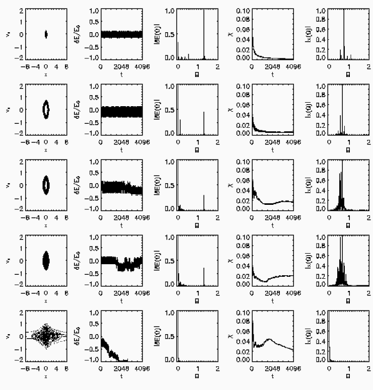
Figure 1: Top row: the phase space trajectory of a typical regular orbit evolved in a triaxial Plummer potential with axis ratios $a^{2}:b^{2}:c^{2}=1.25:1:0.75$, with initial energy $E=-0.8$, $m_{0}=0.1$ and $\omega_{0}=1.3$, along with the relative energy oscillations, $\delta E(t)/E$, the power spectrum $\left|\delta E(\Omega)\right|$, the finite time Lyapunov exponents $\chi$ computed for times $T\leq t$, and the power spectrum, $\left|x(\Omega)\right|$. Second row: the same for a ‘nearly regular’ sticky chaotic orbit, with the peak frequency for $|x({\Omega})|$ satisfying ${\Omega}^{(1)}={\omega}_{0}$ and the peak frequency for $|E({\omega})|$ equally ${\omega}_{0}/2$. Third row: a more irregular sticky orbit which still has the same peak frequencies. Fourth row: a wildly chaotic orbit with spectra peaked at lower frequencies. Fifth row: a more wildly chaotic orbit that rapidly diffuses toward larger radii and lower frequencies.

As noted already, the type of orbit correlates not only with the overall shape of the Fourier spectrum, but with the value of the peak frequencies for which quantities like $|x({\Omega})|$ or $E({\omega})$ have the most power. This is illustrated in Fig. 2, which exhibits scatter plots of ${\chi}$, the largest finite time Lyapunov exponent, and ${\Omega}^{(1)}$, the frequency for which $|x({\Omega})|$ has the most power. Each panel was generated from the same set of $800$ initial conditions. The four columns from left to right correspond to increasing amplitudes $m_{0}=0$, $m_{0}=0.05$, $m_{0}=0.1$, and $m_{0}=0.2$. The driving frequency ${\omega}_{0}=1.3$, and the orbital structure is dominated by a $2:1$ resonance. In particular, for sticky orbits $|x({\Omega})|$ peaks at ${\Omega}^{(1)}={\omega}_{0}/2=0.65$. (By contrast, as is evident from Fig. 1, $|E({\Omega})|$ peaks at ${\Omega}^{(1)}={\omega}_{0}=1.3$.) For all the regular orbits, ${\Omega}^{(1)}$ is larger than ${\omega}_{0}/2$, the value of which is indicated by the vertical dashed line. Alternatively, orbit segments with ${\Omega}^{(1)}\leq{\omega}_{0}/2$ correspond to wildly chaotic orbits.

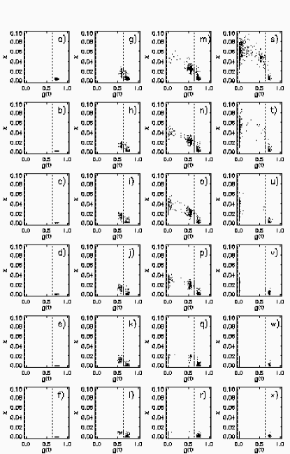
Figure 2: Finite time Lyapunov exponents as a function of peak frequency $\Omega^{(1)}$ for regular ($\Omega^{(1)}>\omega_{0}/2$), sticky ($\Omega^{(1)}\approx\omega_{0}/2$), and wildly chaotic ($\Omega^{(1)}<\omega_{0}/2$) orbits, generated from a microcanonical sampling of 800 initial conditions with energy $E=-0.8$, evolved in a triaxial Plummer potential with $a^{2}:b^{2}:c^{2}=1.25:1:0.75$ and driving frequency $\omega=1.3$, integrated for times $t=1024$, $2048$, $4096$, $8192,$ and $16384$, with amplitudes: (a)-(f) $m_{0}=0$, (g)-(l) $m_{0}=0.05$, (m)-(r) $m_{0}=0.1$, (s)-(x) $m_{0}=0.2$.

For lower amplitude driving, the relative measure of chaotic – as opposed to regular – orbits and the typical size of the largest finite time Lyapunov exponents for the chaotic orbits both tend to be smaller. In particular, for energies and potentials which admit no chaos in the absence of periodic driving, there appears to exist a minimum threshold amplitude, $m_{0}{\;}{\sim}{\;}0.05$, for the onset of appreciable amounts of chaos. For lower amplitudes, the relative measure of sticky chaotic segments – as opposed to wildly chaotic segments – also tends to be higher and, as will be discussed later, in some cases the time required for transitions from sticky to wildly chaotic tends to be longer.

Of especial interest is the case of potentials which, in the absence of periodic driving, admit large measures of both regular and chaotic orbits. As illustrated in Fig. 3, in this case weak driving tends to make some, albeit typically not all, the otherwise regular orbits chaotic; and the already chaotic orbits tend to remain chaotic. Few if any otherwise chaotic orbits are converted to regular. However, it is not true that the driving necessarily increases the values of the largest finite time Lyapunov exponents for all the otherwise chaotic orbits. Indeed, for sufficiently small $m_{0}$ the driving is comparably likely to increase or decrease the value of ${\chi}$. Significantly, though, as $m_{0}$ is increased the degree of chaos always appears to increase, at least initially. For sufficiently large values of $m_{0}$ all the otherwise regular orbits become chaotic and, for the otherwise chaotic orbits, there is a systematic increase in the values of the largest ${\chi}$. However, there will still be a few otherwise chaotic orbits which become less chaotic in the presence of driving. One other obvious trend evident from Fig. 3 is the systematic decrease in the values of ${\chi}(m_{0}{\neq}0)$ at late times. This decrease reflects the fact that the vast majority of the chaotic orbits have become wildly chaotic, and that many of these have drifted to less negative energies, where the orbital time $t_{D}$, and hence the Lyapunov time $1/{\chi}$, is very long.

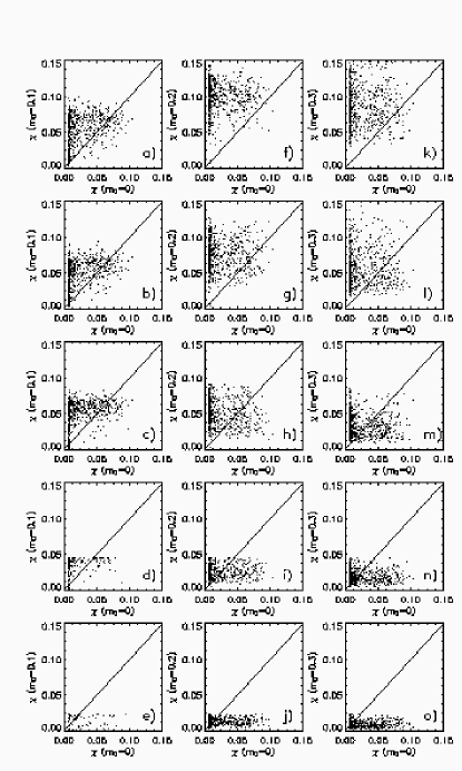
Figure 3: Finite time Lyapunov exponents for driven versus unperturbed orbits, integrated from the same microcanonical set of $800$ initial conditions with $E=-0.8$ in a triaxial Dehnen potential with axis ratios $a^{2}:b^{2}:c^{2}$ $=1.25:1:0.75$ and driving frequency $\omega=2.75$ at varying integration times $t=1024$, $2048$, $4096$, $8192$, and $16384$ for: (a) - (e) $m_{0}=0.1$, (f) - (j) $m_{0}=0.2$ and (k) - (o) $m_{0}=0.3$.

Whether, in the presence of periodic driving, an initial condition results initially in sticky as opposed to wildly chaotic behavior does not appear to correlate strongly with its behavior in the absence of driving. For example, there is no obvious preferential tendency for otherwise regular initial conditions to yield sticky behavior. For a fixed potential, the likelihood that an initial condition yields a sticky, as opposed to wildly chaotic, orbit is determined more by the amplitude $m_{0}$ than by the regular or chaotic behavior exhibited by the initial condition in the absence of periodic driving. When $m_{0}$ is small, sticky orbits tend to be more common; as $m_{0}$ increases, the relative measure of wildly chaotic segments increases.

The relative abundance of different orbit types does not appear to exhibit a simple, universal dependence on shape. In some cases, there is more chaos for parameter values where the equipotential surfaces are oblate and/or prolate, rather than spherical; in others spherical potentials exhibit more chaos. The one trend that does emerge, at least for the models considered here, is that genuinely triaxial potentials with $a{\;}{\neq}{\;}b{\;}{\neq}{\;}c$ tend to exhibit more chaos than potentials with either spherical or spheroidal symmetry.

To quantify at least partially the transition rate between sticky and wildly chaotic behavior, one can, for an orbit ensemble of fixed initial energy, begin by identifying the initial conditions that correspond to chaotic orbits, then identifying the range of energies which, for these initial conditions, correspond to sticky behavior, and finally determining for each orbit generated from a chaotic initial condition the first time that it acquires an energy outside this range. The obvious quantity of interest is the fraction $N(t)/N(0)$ of those chaotic orbits which have not yet ‘escaped’ within time $t$. When, as for the example presented below, the orbital structure is dominated by a $2:1$ resonance, regular orbits can be rejected immediately as having ${\Omega}^{(1)}>{\omega}_{0}/2$. However, the computed fraction does depend somewhat on the precise choice of energy range, which is not completely obvious. Fortunately, though, as discussed below, modest changes do not significantly alter the final results.

Examples of such an analysis, all generated for the same ensemble, are exhibited in Fig. 4, each panel of which plots $N(t)/N(0)$, the relative number of chaotic orbits which are sticky, as a function of time $t$ for different choices of amplitude $m_{0}$. The top two panels are for oblate ($a^{2}=b^{2}=1$, $c^{2}=0.75$) and triaxial ($a^{2}=1.25$, $b^{2}=1$, $c^{2}=0.75$) Plummer potentials which, in the absence of driving, admit few if any chaotic orbits. The lower panels are for oblate and triaxial Dehnen potentials with the same axis ratios, which admit a considerable amount of chaos even in the absence of driving. From this Figure two points are immediately evident. The first is that, in every case, after a very rapid initial decrease, $\ln N$ decreases systematically in a fashion that is roughly linear in time. This implies that, at least in a first approximation, transitions from sticky to wildly chaotic can be viewed a Poisson process,

$$N(t)=N_{0}\exp(-{\Lambda}t),$$ (5)

with $N_{0}$ the number of chaotic orbits which are initially sticky and ${\Lambda}$ the escape rate. This exponential decrease is the same behavior observed for diffusion through cantori in two-degree-of-freedom systems (see, e.g., pk99 ), thus reinforcing again the notion that these transitions involve passage through an entropy barrier.

Figure 4: (a) Fraction $N(t)/N(0)$ of chaotic orbits that remain ‘sticky’ after time $t$, computed for ensembles of $1200$ initial conditions with energy $E=-0.8$, evolved in an oblate Plummer potential with axis ratio $a^{2}:b^{2}:c^{2}=1:1:0.75$, pulsed with frequency ${\omega}_{0}=1.3$ and variable amplitude $m_{0}$. Solid curves with increasing thickness correspond to increasing amplitudes $m_{0}=0.15,0.2,0.25,0.3$. Dashed lines represent best linear fits. (b) The same for a triaxial Plummer potential with $a^{2}:b^{2}:c^{2}=1.25:1:0.75$, again with $E=-0.8$ and ${\omega}_{0}=1.3$. (c) The same for an oblate Dehnen potential with $a^{2}:b^{2}:c^{2}=1:1:0.75$, again with $E=-0.8$ but now with ${\omega}_{0}=2.75$. (d) The same for a triaxial Dehnen potential with $a^{2}:b^{2}:c^{2}=1.25:1:0.75$ with $E=-0.8$ and ${\omega}_{0}=2.75$.

The other striking point is that the dependence of ${\Lambda}$ on $m_{0}$ is very different for the Plummer and Dehnen models. For the Plummer models ${\Lambda}$ is rather nearly independent of driving amplitude; but, for the Dehnen models ${\Lambda}$ increases significantly as $m_{0}$ increases. This is an example of a more general result: If, in the absence of driving, the orbits are all regular, ${\Lambda}$ exhibits little if any dependence on $m_{0}$. If, however, a significant fraction of the orbits are already chaotic in the absence of driving, ${\Lambda}$ is a strongly increasing function of $m_{0}$. The degree of chaos exhibited by a model, as probed by the relative measure of chaotic orbits or the size of a typical finite time Lyapunov exponent, need not correlate especially with the amount of chaos that is present in the absence of driving. However, the presence or absence of chaos in the unperturbed models does impact the transition rate between sticky and wildly chaotic behavior.

But why do plots of $N(t)$ show an initial much more rapid decrease, and how sensitive are these results to the energy range associated with sticky orbit segments? The basic conclusion is that increasing the size of the sticky range slows the early time rapid decrease, but has only a minimal impact on the computed transition rate ${\Lambda}$. The results exhibited in Fig. 4 were computed assuming a range $E_{0}-1.5m_{0}<E<E_{0}+1.5m_{0}$, with $E_{0}$ the initial unperturbed energy and $m_{0}$ the amplitude of the perturbation, but, in most cases, the best fit ${\Lambda}$ changes only by $10\%$ or so if $1.5$ is increased to $3.0$ weird . The validity of this criterion was also tested by comparing the number of orbits that this prescription classifies as sticky at time $t=4096$ with the number of orbits which still appear locked to the driving frequency with ${\Omega}^{(1)}={\omega}_{0}/2$.

The obvious interpretation is that the initial rapid decrease reflects wildly chaotic orbits which require a finite time to escape from the sticky range: if the range is made larger, the time required for escape becomes longer. This suggests in turn that the most accurate estimate of the number of sticky orbits involves assuming the smallest range which clearly includes all sticky orbits, the criterion used to justify a value ${\approx}{\;}1.5$. Given such a choice, one also appears justified in interpreting $N_{0}$ in eq. (2.5) as the relative fraction of the chaotic orbits which are sticky at or near $t=0$.

Given this interpretation of $N_{0}$, one can easily estimate the relative abundance of regular, sticky, and wildly chaotic orbits at time $t=0$. The results for the ensembles used to construct Fig. 4 are exhibited in Fig. 5. It is evident that, in each case, the relative number of chaotic orbits is an increasing function of $m_{0}$, but the relative number of initially sticky orbits can vary significantly. For the Plummer potentials, the relative measure of sticky orbits tends to be very small irrespective of the magnitude of $m_{0}$. For the Dehnen potentials, however, sticky orbits are comparatively common, especially for smaller amplitude driving. In particular, for $m_{0}{\;}{\leq}{\;}0.15$ there are more sticky than wildly chaotic orbits for the oblate Dehnen potential. It should, however, be stressed that the relative measure of sticky versus wildly chaotic model need not increase monotonically as a potential is made less symmetric. For example, ensembles evolved in a spherical Plummer potential perturbed with the same amplitude $m_{0}$ tend to exhibit substantially larger relative measures of sticky orbits.

Figure 5: (a) Relative number of chaotic orbits (solid line and diamonds), sticky chaotic orbits (dashes and squares), and wildly chaotic orbits (dot-dashed lines and triangles) at $t=0$, plotted as a function of $m_{0}$, for the ensembles in Fig. 4, as predicted by the best linear fits.

Assuming that these conclusions are robust, they have obvious implications for chaotic phase mixing in systems subjected to periodic perturbations. Relatively low amplitude periodic driving can suffice to trigger large measures of chaotic orbits. However, these chaotic orbits are apt to be primarily sticky and, as such, unlikely to exhibit large-scale secular changes in energy. In the context of charged-particle beams, this would suggest that periodic driving could facilitate a comparatively rapid loss of coherence, but that it would not necessarily trigger the formation of a halo. If, however, the amplitude of the driving is increased, a larger measure of the orbits will be wildly chaotic; and a substantial fraction of these could drift to higher energy states associated with an extended halo. This expectation is consistent with real experiments involving charged-particle beams (e.g., haber ), which indicate that particle bunches which undergo larger amplitude oscillations (larger initial ‘mismatch’) tend to form more extended halos.

III LOW AMPLITUDE NOISE

The objective now is to describe how distinctions amongst regular, sticky chaotic, and wildly chaotic behavior and, especially, the rate of transitions between sticky and wildly chaotic behavior, are impacted by the introduction of weak perturbations, modeled as friction and/or Gaussian noise. The conclusions derive from an analysis of orbits generated as solutions to the perturbed evolution equation

$${d^{2}x^{i}\over dt^{2}}=-{{\partial}V\over{\partial}x^{i}}-{\eta}{dx^{i}\over dt}+F^{i}(t).$$ (6)

Here ${\eta}dx^{i}/dt$ represents a dynamical friction and $F^{i}$ is a Gaussian-distributed random force which, for specificity, is assumed to sample an Ornstein-Uhlenbeck process.

In the context of a galaxy or charged-particle beam, random perturbations associated with an external environment could correspond vanK to extrinsic noise, for which ${\eta}{\;}{\equiv}{\;}0$. Alternatively, effects associated with graininess or internal substructures could correspond to intrinsic noise, with a nonzero ${\eta}$ related to the moments of $F^{i}$ by the Fluctuation-Dissipation Theorem. In particular, the effects of graininess can be modeled (see, e.g., sk02 ) as intrinsic white noise, which can be viewed as a singular limit of an Ornstein-Uhlenbeck process with vanishing autocorrelation time.

The assumption that $F^{i}$ is Gaussian noise sampling an Ornstein-Uhlenbeck process implies that the stochastic process is characterized completely by its first two moments,

$${\langle}F^{i}(t){\rangle}=0\qquad{\rm and}$$

$${\langle}F^{i}(t_{1})F^{j}(t_{2}){\rangle}={\delta}^{ij}\;K(|t_{1}-t_{2}|),$$ (7)

where ${\langle}\;.\;{\rangle}$ denotes a statistical average and the autocorrelation function $K$ satisfies

$$K(|t_{1}-t_{2}|)={\Delta}^{2}\exp(-|t_{1}-t_{2}|/t_{c}).$$ (8)

Here ${\Delta}$ represents the typical ‘size’ of the random force and the autocorrelation time $t_{c}$ the time scale over which it changes appreciably. The limit $t_{c}\to 0$ corresponds to white noise. State-independent, additive noise has ${\eta}$ and $K$ independent of phase space coordinates. Multiplicative noise arises when these quantities are functions of $x^{i}$ and/or $v^{i}$.

Three different variants were considered:

1. Additive noise, both white and colored, without friction.

2. Additive noise with friction related by the Fluctua-tion-Dissipation Theorem,

$$\int_{-\infty}^{+\infty}d{\tau}K({\tau})=2{\Theta}{\eta}{\;}{\equiv}{\;}D,$$ (9)

where ${\Theta}$ represents a temperature and $D$ the diffusion constant entering into a Fokker-Plank description vanK . (This implies ${\Delta}^{2}={\Theta}{\eta}/t_{c}$.) On physical grounds, ${\Theta}$ was typically selected to be comparable in magnitude to the initial energy of the orbit(s) in question.

3. Multiplicative noise with $K(v^{i})$ satisfying

$$K(v^{i})=K_{0}v^{2}/{\langle}v^{2}{\rangle},$$ (10)

with $K_{0}$ the autocorrelation function appropriate for additive noise, $v^{2}$ the squared speed of the orbit, and ${\langle}v^{2}{\rangle}$ the mean squared speed of an orbit with the specified initial energy.

There is no uniformly accepted definition of chaos or Lyapunov exponent for stochastic differential equations. However, the following prescription, implemented in this paper, appears to capture one’s physical intuition in terms, e.g., of the visual appearance of an orbit. Specifically, in the context of this paper ${\chi}$ will be defined in the usual way by comparing the evolution of two nearby initial conditions, assuming, however, that both orbits feel exactly the same noise and, for consistency, the same friction. This entails solving a perturbation equation

$${d^{2}{\delta}x^{i}\over dt^{2}}=-{{\partial}^{2}V\over{\partial}x^{i}{\partial}x^{j}}{\delta}x^{j},$$ (11)

where the Hessian is evaluated along the original noisy orbit. This prescription obviates the necessity of deciding how to relate concrete realizations of a stochastic process at two nearby phase space points.

Consider first the effects of white noise. If, in the absence of noise, most of the orbits are not already chaotic, the most conspicuous effect resulting from the addition of noise is to increase the relative abundance of chaotic orbits. This is, for example, illustrated in Fig. 6, generated for the same Plummer models used to produce Fig. 4, which exhibits the relative measure $f_{c}$ of chaotic orbits as a function of amplitude ${\eta}$. For all three choices of $m_{0}$, the noise has a discernible effect even for amplitudes as small as ${\eta}=10^{-7}$; for ${\eta}$ as large as $10^{-4}$ almost all the orbits have become chaotic. Interestingly, however, the noise does not have a significant impact on the size of a typical finite time Lyapunov exponent for those orbits which are chaotic.

Figure 6: Relative measure of chaotic orbits, $f_{c}$, computed for a microcanonical ensemble of $1200$ initial conditions with energy $E=-0.8$ in a pulsating triaxial Plummer potential with axis ratio $a^{2}:b^{2}:c^{2}=1.25:1:0.75$, evolved with $\omega_{0}=1.3$, $m_{0}=0.1$ (empty circles with solid line), $m_{0}=0.15$ (crosses with short-dashed line), $m_{0}=0.2$ (asterisks with long-dashed line) and $m_{0}=0.3$ (filled circles with dash-dotted line) in the presence of additive white noise with ${\Theta}=1.0$ and variable amplitude ${\eta}$.

The empirical distinction between sticky and wildly chaotic orbits persists in the presence of relatively low amplitude noise, and transitions between sticky and wildly chaotic still appear to sample a (near-)Poisson process. However, as was the case in the absence of noise, the observed behavior of orbit ensembles depends considerably on whether or not the orbits are almost all chaotic.

For systems like the Plummer potentials, where there is little chaos in the absence of driving, the rate ${\Lambda}$ associated with transitions between sticky and wildly chaotic is largely independent of ${\eta}$. Increasing the noise amplitude, which increases the overall abundance of chaotic orbits, also increases the abundance of initially sticky chaotic segments; but the rate at which these are transformed into wildly chaotic orbits is largely unaffected unless the noise becomes very large in amplitude.

Alternatively, for systems like the Dehnen potentials, where there is a good deal of chaos even in the absence of driving, the addition of noise definitely accelerates transitions from sticky to wildly chaotic. This is, e.g., illustrated in the left hand column of Fig. 7, which exhibits $N(t)/N(0)$, the relative number of orbit that are still sticky, for the triaxial Dehnen potential used to generate Fig. 4. The qualitative behavior manifested in these panels is very similar to that associated with diffusion through cantori in two-degree-of-freedom Hamiltonian systems (cf. pk99 ), where one can argue that, by wiggling orbits, ‘noise helps orbits find holes’ in entropy barriers.

Figure 7: (a) Fraction $N(t)/N(0)$ of chaotic orbits that remain ‘sticky’ after time $t$, computed for ensembles of $1200$ initial conditions with $E=-0.8$, evolved in a triaxial Dehnen potential with axis ratio $a^{2}:b^{2}:c^{2}=1.25:1:0.75$, ${\omega}_{0}=2.75$, and $m_{0}=0.1$, allowing for additive white noise with variable amplitude. Dashed lines correspond to integrations without white noise, while the magnitude of $\eta$ increases with increasing line thickness through values $\eta=10^{-7},10^{-6},10^{-5},10^{-4}$. In each case ${\Theta}=1$. (b) The mean energy ${\langle}E(t){\rangle}$ computed for the same ensemble. (c) and (d) The same for $m_{0}=0.15$.

The situation for larger amplitude noise is rather different. Seemingly independent of the form of the potential, for ${\eta}>10^{-3}-10^{-2}$ escapes happen so quickly that the distinction between sticky and wildly chaotic becomes essentially meaningless. This can be understood by observing that, when the noise has such a large amplitude, it will pump energy into the orbit so rapidly that, even if the driving has a relatively minimal effect, one cannot think of the orbit as being restricted to a nearly constant energy hypersurface.

Although these conclusions were derived allowing only for additive white noise in the absence of any dynamical friction, they appear to be comparatively insensitive to the form of the perturbation. For example, the presence or absence of a dynamical friction of comparable amplitude ${\eta}$ is largely irrelevant. Moreover, there is no indication that allowing for ‘generic’ multiplicative noise would alter the basic picture. For example, allowing for multiplicative noise with an autocorrelation function scaling as in eq. (3.5) has only a minimal effect on the relative number of chaotic orbits or the transition rate between sticky and wildly chaotic behavior. All that really seems to matter is the amplitude of the noise. Moreover, even this dependence on amplitude is comparatively weak. Inspection of Figs. 6 and 7 indicates that there is only a roughly logarithmic dependence on ${\eta}$.

Also of interest is how the combined effects of periodic driving and friction/noise impact the mean energies of typical particle orbits. Examples of such behavior, again computed for orbits in a pulsed, triaxial Dehnen potential perturbed only by additive white noise, are exhibited in the right hand column of Fig. 7.

But how are such data to be interpreted? It follows immediately from the Langevin equation (3.1) that, allowing only for periodic driving and additive white noise, the mean energy ${\langle}E{\rangle}$ associated with some ensemble will satisfy

$${d{\langle}E{\rangle}\over dt}=\left\langle{{\partial}V\over{\partial}t}\right\rangle+3{\Theta}{\eta},$$ (12)

where ${\langle}{\partial}V/{\partial}t{\rangle}$ represents an average computed along the orbits. The noise leads directly to a linear increase in energy at a constant rate $3{\Theta}{\eta}$, independent of the form of the driving; the driving occasions an additional increase which will in general depend on the form of the perturbed orbits. Given the mean value ${\langle}E(t){\rangle}$ computed for orbits that are subjected to both noise and periodic driving, it is thus natural to subtract off the linear increase $3{\Theta}{\eta}t$ directly attributable and to compare the residual with the mean ${\langle}E(t){\rangle}$ computed in the absence of noise. To the extent that the former quantity is larger, one can infer that noise enhances the energy diffusion associated with periodic driving in the sense that the mean change in energy is larger than what would obtain allowing only for the separate effects of driving and noise.

The results of such an analysis are exhibited in Fig. 8, each panel of which plots the quantity

$${\Delta}V=\int{\langle}{\partial}V/{\partial}t{\rangle}~{}dt,$$ (13)

derived for the same set of initial conditions, evolved in the same potential with the same amplitude $m_{0}$ and same ${\omega}_{0}$ but in the presence of additive white noise with different amplitudes ${\eta}$. For both the Plummer and Dehnen potentials, it is evident that, at least for low amplitudes $m_{0}$, increasing ${\eta}$ tends to increase ${\Delta}V$, i.e., that the noise and driving reinforce one another in a superadditive fashion. However, for higher amplitudes $m_{0}$, more variability is observed, the one uniform feature being that the relative degree of reinforcement is less. In this sense, one can say that noise is more important as a source of energy diffusion in systems subjected to relatively low amplitude driving.

Figure 8: Mean value of the quantity ${\Delta}V$, as defined in 13, computed for $1200$ orbits with initial energy $E=-0.8$ evolved in a pulsating triaxial Plummer potential with axis ratio $a^{2}:b^{2}:c^{2}=1.25:1:0.75$, ${\omega}_{0}=1.3$, and variable amplitude (a) $m_{0}=0.1$ and (b) $m_{0}=0.2$. Dashed lines correspond to integrations without white noise, while the magnitude of white noise $\eta$ increases with increasing line thickness through values $\eta=10^{-7},10^{-6},10^{-5},10^{-4}$. (c) - (d) The same for a triaxial Dehnen potential with axis ratio $1.25:1:0.75$, and ${\omega}_{0}=2.75$.

But how is all this effected by allowing for colored noise with a finite autocorrelation time? If the autocorrelation time $t_{c}$ is sufficiently short compared with the dynamical time, colored noise has virtually the same effect as white noise. However, when $t_{c}$ becomes comparable to the orbital time $t_{D}$ the effects of the noise become weaker; and, for $t_{c}$ sufficiently large compared with $t_{D}$ the noise has only a relatively minimal effect.

Figure 9 illustrates how, for the same initial conditions used to generate Fig. 6, the relative number $f_{c}$ of chaotic orbits depends on both amplitude ${\eta}$ and autocorrelation time $t_{c}$. The top panel illustrates clearly that, for fixed ${\eta}$, increasing $t_{c}$ reduces the degree to which the noise converts regular orbits to chaotic. However, it is also apparent that, for sufficiently large ${\eta}$, almost all the orbits still become chaotic. The autocorrelation time must assume a value even larger than $t_{c}=32$ if the effects of the noise are to ‘turn off’ almost completely for amplitudes as large as ${\eta}=10^{-4}$.

Figure 9: Relative measure of chaotic orbits, $f_{c}$, computed for a microcanonical ensemble of $800$ initial conditions with energy $E=-0.8$ in a pulsating triaxial Plummer potential with axis ratio $a^{2}:b^{2}:c^{2}=1.25:1:0.75$, evolved with frequency ${\omega}_{0}=1.3$ and $m_{0}=0.1$ in the presence of noise with varying amplitude ${\eta}$ and autocorrelation time $t_{c}$. In (a): solid line with empty circles represents white noise (limit $t_{c}\to 0$), short-dashed line with crosses $t_{c}=0.5$, long-dashed line with squares $t_{c}=2$, and dash-dot line with triangles $t_{c}=8$, dash-dot-dot-dot line with filled circles $t_{c}=32$. In (b): solid line with empty circles represents $\eta=10^{-7}$, short-dashed line with crosses $\eta=10^{-6}$, long-dashed line with squares $\eta=10^{-5}$, dash-dot line with triangles $\eta=10^{-4}$, dash-dot-dot-dot line with filled circles $\eta=10^{-3}$. Horizontal dashed line corresponds to the fraction of chaotic orbits for the same ensemble evolved in the absence of any noise.

The panel a) of Fig. 10, generated for orbits in triaxial Plummer, demonstrate that the rates of transition between sticky and wildly chaotic behavior are largely independent of the autocorrelation time $t_{c}$. The panel c) of Fig. 10, representing orbits in triaxial Dehnen potentials, show that increasing the autocorrelation time $t_{c}$ tends also to weaken the effects of noise in accelerating transitions between sticky and wildly chaotic behavior.

Figure 10: (a) Fraction $N(t)/N(0)$ of chaotic orbits that remain ‘sticky’ after time $t$, computed for ensembles of $800$ initial conditions with $E=-0.8$, evolved in a triaxial Plummer potential with axis ratio $a^{2}:b^{2}:c^{2}=1.25:1:0.75$, ${\omega}_{0}=1.3$, and $m_{0}=0.1$, allowing for colored noise with ${\eta}=10^{-4}$ and variable $t_{c}$. The magnitude of $t_{c}$ increases with increasing line thickness through values $t_{c}=0.5$, $1$, $2$, and $4$. The long-dashed line corresponds to white noise. The short-dashed line corresponds to the same ensemble evolved in the absence of any kind of noise. (b) The mean energy ${\langle}E(t){\rangle}$ computed for the same ensembles. (c) and (d) The same for ensembles evolved in a triaxial Dehnen potential with $a^{2}:b^{2}:c^{2}=1.25:1:0.75$ and ${\omega}_{0}=2.75$, again with $m_{0}=0.1$ and ${\eta}=10^{-5}$.

The panels b) and d) of Fig. 10, generated for the same initial conditions, demonstrates that increasing autocorrelation time $t_{c}$ decreases the rates of the mean change in energy. For both potentials, the curve for $t_{c}=0.5$ coincides very nearly with the white noise curve, and the appreciable decreases in ${\langle}E(t){\rangle}$ arise for $t_{c}{\;}{\geq}{\;}1.0$.

IV FREQUENCY VARIATIONS

The objective now is to explore how the results described in the preceding Section are altered if one allows instead for variations in the pulsation frequency, again modeled as Gaussian noise sampling an Ornstein-Uhlenbeck process. What this entails is allowing for a variable frequency ${\omega}(t)={\omega}_{0}+{\delta}{\omega}(t)$, where the random frequency shift ${\delta}{\omega}$ is characterized by moments

$${\langle}{\delta}{\omega}(t){\rangle}=0$$

and

$${\langle}{\delta}{\omega}(t_{1}){\delta}{\omega}(t_{2}){\rangle}={\Omega}^{2}\exp(-|t_{1}-t_{2}|/t_{c}).$$ (14)

This implies in particular that ${\langle}{\omega}^{2}(t){\rangle}={\omega}_{0}^{2}+{\Omega}^{2}$. The form of the experiments was the same as in the preceding Section. The computations were performed assuming $F^{i}={\eta}=0$, i.e no ordinary noise.

As discussed in the preceding Section, allowing for ‘ordinary’ white noise tends to increase the relative abundance of chaotic orbits, especially for systems which, in the absence of driving, admit few if any chaotic orbits. Allowing for a ‘noisy’ frequency with vanishing autocorrelation time has exactly the opposite effect. For systems where, in the absence of driving, little if any chaos is present, making the frequency ‘stutter’ by introducing even comparatively low amplitude white noise impulses tends instead to decrease the relative abundance of chaotic orbits. This is, e.g., evident from Fig. 11, which was generated for the same initial conditions as Fig. 6, now allowing for white noise variations in ${\omega}$ with different amplitudes ${\Omega^{2}}$.

Figure 11: Relative measure of chaotic orbits, $f_{c}$, computed for a microcanonical ensemble of $800$ initial conditions with energy $E=-0.8$ in a pulsating triaxial Plummer potential with axis ratio $a^{2}:b^{2}:c^{2}=1.25:1:0.75$, evolved with ${\omega}_{0}=1.3$, $m_{0}=0.1$ (empty circles with solid line), $m_{0}=0.15$ (crosses with short-dashed line), $m_{0}=0.2$ (asterisks with long-dashed line) and $m_{0}=0.3$ (filled circles with dash-dotted line), allowing for ‘white noise’ random variations in frequency with variable amplitude ${\Omega^{2}}$.

As is illustrated in Fig. 12, allowing for random variations in frequency tends also to suppress transitions from sticky to wildly chaotic behavior and to decrease the amount of energy that the driving can pump into the orbits. White noise variations in frequency dramatically reduce the effects of driving as a source of energy diffusion.

Figure 12: Fraction $N(t)/N(0)$ of chaotic orbits that remain ‘sticky’ after time $t$, computed for ensembles of $800$ initial conditions with $E=-0.8$, evolved in a triaxial Dehnen potential with axis ratio $a^{2}:b^{2}:c^{2}=1.25:1:0.75$, ${\omega}_{0}=2.75$, and $m_{0}=0.1$, allowing for ‘white noise’ variations in frequency with variable amplitude ${\Omega}$. The magnitude of the noise increases with increasing line thickness through values ${\Omega^{2}}=10^{-7}$, $10^{-6}$, $10^{-5}$, and $10^{-4}$. The dashed line corresponds to integrations without frequency variations. (b) The mean energy ${\langle}E(t){\rangle}$ computed for the same ensembles. (c) and (d) The same for $m_{0}=0.2$.

These differences are reflected by the fact that even very weak perturbations, with amplitudes as small as ${\Omega^{2}}=10^{-6}$, completely alter the Fourier spectra of the orbits. Examples thereof are provided in Fig. 13 for both triaxial Plummer and triaxial Dehnen potentials. In each case, it is evident that, in the absence of the perturbation, there is a dominant resonance, ${\Omega}^{(1)}=\omega_{0}/2=0.65$ for the Plummer potential and ${\Omega}^{(1)}=\omega_{0}/2=1.375$ for the Dehnen potential. But, in each case, it is also apparent that, even for noise as weak as ${\Omega^{2}}=10^{-5}$, the effects of this resonance have entirely disappeared.

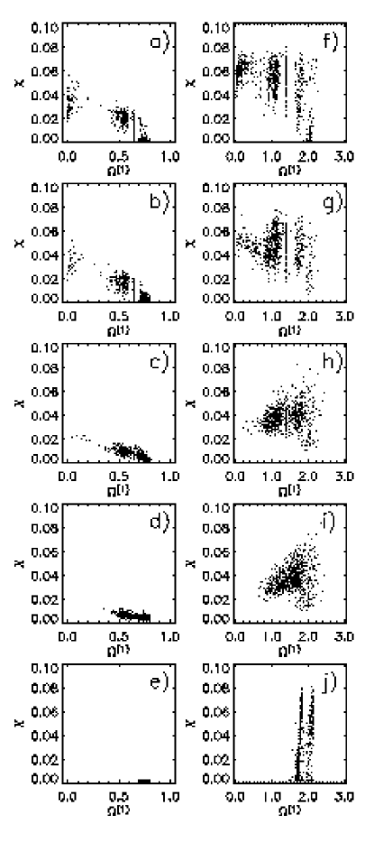
Figure 13: Finite time Lyapunov exponent as a function of frequency $\Omega^{(1)}$ for $800$ orbits with initial energy $E=-0.8$ in a triaxial Plummer potential with axis ratio $a^{2}:b^{2}:c^{2}=1.25:1:0.75$, pulsating with amplitude $m_{0}=0.1$ and $\omega_{0}=1.3$, allowing for ‘white noise’ variations with (a) ${\Omega}=0$, (b) ${\Omega^{2}}=10^{-7}$, (c) ${\Omega}=10^{-6}$, and (d) ${\Omega}=10^{-5}$. (e) The same ensemble evolved in the absence of both noise and driving. (f) - (j) The same for orbits in a Dehnen potential with ${\omega}_{0}=2.75$, again with $a^{2}:b^{2}:c^{2}=1.25:1:0.75$ and $m_{0}=0.1$.

Also evident from this Figure is the fact that even a very small ${\Omega^{2}}$ suffices to prevent orbits from diffusing to very large energy. In the absence of frequency variations, both potentials admit orbits that diffuse towards very large radii and, consequently, have very small peak frequencies. However, for ${\Omega^{2}}>10^{-5}$, there are no orbits with ${\Omega}^{(1)}<0.4$. This does not, however, necessarily imply that there are no chaotic orbits at all. For the case of the Dehnen potential there are still significant numbers of chaotic orbits with larger values of ${\Omega}^{(1)}$.

One might naively have expected that the stuttering simply ‘turns off’ the effects of the driving, so that orbits pulsed with $m_{0}=0.1$ and ${\Omega^{2}}=10^{-7}$, $10^{-6}$, or $10^{-5}$ behave very much like orbits evolved with $m_{0}={\Omega^{2}}=0$. This, however, is not the case. It is, for example, clear that, for the Dehnen model, the distribution of peak frequencies for an unpulsed, constant frequency integration has far more structure than the distributions for the pulsed, variable frequency models. Even though frequency variations can dramatically reduce the efficacy of the driving as a source of energy diffusion, they do not transform orbits back to the form they had in the absence of driving.

Adding color strengthens the effects of the perturbation. An example of this tendency is illustrated in Fig. 14, which exhibits the fraction of chaotic orbits for the ensembles of $800$ orbits in a pulsed Plummer potential, allowing for random variations in frequency with different values of ${\Omega^{2}}$ and $t_{c}$. It is clear from the bottom panel that increasing the value of autocorrelation time from the $t_{c}\to 0$ white noise limit results in a systematic increase in the relative measure of chaotic orbits. Also evident is the fact that even a relatively small value $t_{c}=0.5$ is sufficient to significantly increase the number of chaotic orbits relative to the white noise limit. As is evident from the lower panel, in the long autocorrelation time limit, $t_{c}\to\infty$, the effects of the colored noise gradually turn off. This is to be expected, if one views $t_{c}\to\infty$ as an adiabatic limit. The time-scale on which this turning off occurs is directly proportional to the amplitude of colored noise, i.e, it takes longer autocorrelation times for the effects of the stronger noise to reach the adiabatic limit.

Figure 14: Relative measure of chaotic orbits, $f_{c}$, computed for a microcanonical ensemble of $800$ initial conditions with energy $E=-0.8$ in a pulsating triaxial Plummer potential with axis ratio $a^{2}:b^{2}:c^{2}=1.25:1:0.75$, evolved with frequency ${\omega}_{0}=1.3$ and $m_{0}=0.1$, allowing for ‘colored noise’ variations in frequency with variable amplitude ${\Omega^{2}}$ and autocorrelation time $t_{c}$. In (a): solid line with empty circles represents white noise (limit $t_{c}\to 0$), short-dashed line with crosses $t_{c}=0.5$, long-dashed line with squares $t_{c}=2$, and dash-dot line with triangles $t_{c}=8$, dash-dot-dot-dot line with filled circles $t_{c}=32$. In (b): solid line with empty circles represents $\Omega^{2}=10^{-7}$, short-dashed line with crosses $\Omega^{2}=10^{-6}$, long-dashed line with squares $\Omega^{2}=10^{-5}$, dash-dot line with triangles $\Omega^{2}=10^{-4}$, dash-dot-dot-dot line with filled circles $\Omega^{2}=10^{-3}$. Horizontal dashed line corresponds to the fraction of chaotic orbits for the same ensemble evolved in the absence of any noise.

The left panel of Fig. 15 illustrates the fact that allowing for a finite autocorrelation time enhances the transitions from sticky to wildly chaotic behavior. The right hand panel illustrates the fact that, for fixed amplitude ${\Omega^{2}}$, integrations with nonvanishing autocorrelation time $t_{c}$ will pump more energy into the orbits than corresponding integrations with white noise or in the absence of noise. The observed approach of the thick solid lines representing large autocorrelation time $t_{c}$ to the short-dashed lines corresponding to integrations in the absence of any noise illustrates that the effects of the noise are turning off in the $t_{c}\to\infty$ limit.

Figure 15: (a) Fraction $N(t)/N(0)$ of chaotic orbits in a $800$ orbit ensemble that remain ‘sticky’ after time $t$, computed for an ensemble of initial conditions with $E=-0.8$, evolved in a pulsating triaxial Dehnen potential with axis ratio $a^{2}:b^{2}:c^{2}=1.25:1:0.75$, ${\omega}_{0}=2.75$ and $m_{0}=0.1$, allowing for ‘colored noise’ random variations in frequency with ${\Omega^{2}}=10^{-5}$ and variable $t_{c}$. The magnitude of $t_{c}$ increases with increasing line thickness through values $t_{c}=0.5$, $2$, $8$, and $32$. The long-dashed line corresponds to white noise. The short-dashed line corresponds to the same ensemble evolved in the absence of any kind of noise. (b) The mean energy ${\langle}E(t){\rangle}$ computed for the same ensembles.

One other point would seem significant. For the case of ‘ordinary’ noise, incorporated as a random force in the equations of motion, typically a comparatively large autocorrelation time $t_{c}{\;}{\approx}{\;}1$ is required before one sees appreciable differences from the white noise limit. By contrast, however, for the case of ‘noisy’ variations in frequency even an autocorrelation time as small as $t_{c}=0.5$ yields substantial differences from the white noise limit.

V CONCLUSIONS

Orbits in three-dimensional potentials subjected to periodic driving, $V(x^{i},t)=(1+m_{0}\sin{\omega}t)V_{0}(x^{i})$, divide into two distinct types, between which transitions are seemingly impossible: regular orbits, which are strictly periodic and have vanishing Lyapunov exponents, and chaotic orbits, which are aperiodic and have at least one positive Lyapunov exponent. Viewed over finite time intervals, the chaotic orbits divide in turn into two types: ‘sticky’ chaotic segments, which are locked to the driving frequency and exhibit little systematic energy diffusion, and ‘wildly chaotic’ segments, which are not so locked and can exhibit significant energy diffusion. The latter distinction is not absolute, transitions between sticky and wildly chaotic apparently involving motion through entropy barriers.

The relative abundance of sticky versus wildly chaotic segments depends considerably on the form of the potential. However, sticky segments tend overall to be more common for low amplitude driving, i.e., the relative phase space measure associated with sticky orbits tends to be larger. Increasing the amplitude also tends to increase the transition rate between sticky and wildly chaotic behavior, which suggests that the ‘holes’ associated with the entropy barriers become larger as $m_{0}$ increases.

The properties of orbits in such time-periodic potentials can be impacted significantly even by very low amplitude perturbations, both random impulses added to the equations of motion and random variations in the driving frequency, in each case modeled as Gaussian noise sampling an Ornstein-Uhlenbeck process. For fixed amplitude of the perturbation, the largest effects arise in the white noise limit of vanishing autocorrelation time $t_{c}$ and decrease systematically with increasing $t_{c}$. The details of the perturbation tend to be comparatively unimportant. For example, for the case of ‘ordinary’ noise the presence or absence of friction of comparable magnitude and/or making the noise multiplicative as opposed to additive has a comparatively minimal effect. Even the precise strength of the perturbation is relatively unimportant, the response exhibiting only a weak, roughly logarithmic dependence on amplitude.

Ordinary noise tends to enhance the effects of periodic driving by increasing the relative measure of chaotic orbits, especially in potentials which contain little if any chaos in the absence of driving. It also acts to accelerate transitions between sticky and wildly chaotic behavior, thus facilitating more efficient energy diffusion. The effects of noise in frequencies of pulsations have more complex effects. White noise suppresses the effects of periodic driving by decreasing transitions between sticky and wildly chaotic behavior. Colored noise fluctuations, at least for autocorrelation times on the order of the dynamical time, enhances the effects of periodic driving. These effects gradually turn off in the adiabatic $t_{c}\to\infty$ limit.

Ordinary noise appears to act by enhancing the effects of the resonances associated with the periodic driving. Wiggling orbital trajectories can allow an otherwise regular orbit to be impacted by a resonance which it might not otherwise ‘feel’, thus causing it to become chaotic. And similarly, the accelerated rate of transitions between sticky and wildly chaotic behavior can be attributed to the fact that such wiggling helps already chaotic orbits ‘find’ holes in the entropy barrier. Indeed, the effect of noise in enhancing such transitions is very similar qualitatively to the effect of noise as a source of accelerated diffusion through cantori in time-independent two-degree-of-freedom Hamiltonian systems pk99 .

Random white noise variations in the driving frequency appear to weaken the resonances. Making the frequency ‘stutter’ by adding even a very low amplitude, high frequency component to the driving significantly alters the Fourier spectra of orbits, suppressing structure which, in the absence of the perturbation, indicates the importance of the resonances. Variations characterized by non-vanishing autocorrelation time enhances the resonances because the Fourier spectrum of the frequency now has another strong component with which the fundamental frequencies of orbits can resonate.

Appendix A Implementing White and Colored Noise

Here we outline the implementation of noisy equations of motion (6). The term $F^{i}(t)$ is a Gaussian-distributed random force which samples Ornstein-Uhlenbeck process. It has a autocorrelation time $t_{c}$, which in the limit $t_{c}\to 0$ samples ordinary white noise. $F^{i}(t)$ is a normalized solution to the free particle Langevin equation

$${{du^{i}}\over{dt}}+{1\over t_{c}}u^{i}={1\over t_{c}}w^{i}(t),$$ (15)

where $w^{i}(t)$ is Gaussian-distributed white noise with zero mean and unit variance. It is well known that such a variable is easily generated as a sum of 12 random numbers in the range $[-1/2,1/2]$. The solution to (15) is given by uo

$$u^{i}(t)= u^{i}_{0} ~{}\exp(-t/t_{c})$$ (16)

$$+ {1\over t_{c}}~{}\exp(-t/t_{c})\int\limits_{0}^{t}\exp(\xi/t_{c})~{}w^{i}(\xi)~{}d\xi,$$

which, after some straightforward algebra, yields

$$\langle{{u^{i}}^{2}}\rangle={1\over{2t_{c}}}+\left({{u_{0}}^{i}}^{2}-{1\over{2t_{c}}}\right)\exp(-2t/t_{c}).$$ (17)

The second term is transient, so that for $t\gg t_{c}$,

$$\langle{{u^{i}}^{2}}\rangle\approx{1\over{2t_{c}}}.$$ (18)

This means that the random variable $\sqrt{2t_{c}}{~{}\!}u^{i}$ has autocorrelation time $t_{c}$, zero mean and unit variance.

We determine the proper amplitude of colored noise $A$ after substituting $F^{i}(t)=\sqrt{A}{~{}\!}u^{i}(t)$, into the equation (7) and equating it with the equation (8):

$$\langle F^{i}(t_{1})F^{j}(t_{2})\rangle = {A\over{2t_{c}}}\exp(-|t_{1}-t_{2}|/t_{c})$$ (19)

$$= \Delta^{2}\exp(-|t_{1}-t_{2}|/t_{c})$$

$$= {D\over{2t_{c}}}\exp(-|t_{1}-t_{2}|/t_{c}),$$

from which it is clear that $A=D\equiv 2\Theta\eta$. Therefore, the properly scaled noise noise factors are $F^{i}(t)=\sqrt{2\Theta\eta}{~{}\!}u^{i}(t)$, where $u^{i}(t)$ is the solution of (15) for colored noise, and $F^{i}(t)=\sqrt{2\Theta\eta}{~{}\!}w^{i}(t)$, where $w^{i}(t)$ is Gaussian-distributed white noise with zero mean and unit variance.