Dynamical properties of a family of collisionless models of elliptical galaxies

Abstract

N-body simulations of collisionless collapse have offered important clues to the construction of realistic stellar dynamical models of elliptical galaxies. Such simulations confirm and quantify the qualitative expectation that rapid collapse of a self-gravitating collisionless system, initially cool and significantly far from equilibrium, leads to incomplete relaxation, that is to a quasi-equilibrium configuration characterized by isotropic, quasi-Maxwellian distribution of stellar orbits in the inner regions and by radially biased anisotropic pressure in the outer parts. In earlier studies, as illustrated in a number of papers several years ago (see ber93 and references therein), the attention was largely focused on the successful comparison between the models (constructed under the qualitative clues offered by the N-body simulations mentioned above) and the observations. In this paper we revisit the problem of incomplete violent relaxation, by making a direct comparison between the detailed properties of a family of distribution functions and those of the products of collisionless collapse found in N-body simulations.

1 Introduction

We examine the results of a set of simulations of collisionless collapse of a stellar system and focus on the fit of the final quasi-equilibrium configurations by means of the so-called $f^{(\nu)}$ models (see sti87 , ber03 ). The models, constructed on the basis of theoretical arguments suggested by statistical mechanics, are associated with realistic luminosity and kinematic properties, suitable to represent elliptical galaxies. All the simulations have been performed using a new version tren04 of the original code of van Albada (see van82 ; the code evolves a system of simulation particles interacting with one another via a mean field calculated from a spherical harmonic expansion of a smooth density distribution), starting from various initial conditions characterized by approximate spherical symmetry and by a small value of the virial parameter $u$ ($u=-2K/W<0.2$; here $K$ and $W$ represent total kinetic and gravitational energy). From such initial conditions, the collisionless “gravitational plasma” evolves undergoing incomplete violent relaxation lyn67 .

The models, in spite of their simplicity and of their spherical symmetry, turn out to describe well and in detail the end products of our simulations. We should note that the present formulation neglects the presence of dark matter. Since there is convincing evidence for the presence of dark matter halos also in elliptical galaxies, this study should be extended to the case of two-component systems, before a satisfactory comparison with observed galaxies can eventually be claimed.

2 N-body experiments

Most simulations have been run with $8\times 10^{5}$ particles; the results have been checked against varying the number of particles. The units chosen are $10^{11}~{}M_{\odot}$ for mass, $10~{}kpc$ for length, and $10^{8}~{}yr$ for time. In these units the gravitational constant is $G\approx 4.497$, the mass of the model is $2$, and the initial radius of the system $1$.

We focus on clumpy initial conditions. These turn out to lead to more realistic final configurations (van82 , lon91 ). They can be interpreted as a way to simulate the merging of several smaller structures to form a galaxy. The clumps are uniformly distributed in space, within an approximate spherical symmetry; the ellipticity at the beginning of the simulation is small, so that the corresponding initial shape would resemble that of $E2-E3$ galaxies. We performed several runs varying the number of clumps and the virial ratio $u$ in the range from $0.05$ to $0.2$. Usually the clumps are cold, i.e. their kinetic energy is all associated with the motion of their center of mass.

The simulations are run up to time $t=10$, when the system has settled into a quasi-equilibrium. The violent collapse phase takes place within $t\approx 1$ . The final configurations are quasi-spherical, with shapes that resemble those of $E2-E3$ galaxies. The final equilibrium half-mass radius $r_{M}$ is basically independent of the value of $u$. The central concentration achieved is a function of the initial virial parameter $u$, as can be inferred from the conservation of maximum density in phase space lon91 .

3 Physically justified models

For a spherically symmetric kinetic system, extremizing the Boltzmann entropy at fixed values of the total mass, of the total energy, and of an additional third quantity $Q$, defined as $Q=\int J^{\nu}|E|^{-3\nu/4}fd^{3}qd^{3}p$, leads (sti87 ; see also ber03 ) to the distribution function $f^{(\nu)}=A\exp{[-aE-d(J^{2}/|E|^{3/2})^{\nu/2}]}$, where $a$, $A$, $d$, and $\nu$ are positive real constants; here $E$ and $J$ denote single-star specific energy and angular momentum. At fixed value of $\nu$, one may think of these constants as providing two dimensional scales (for example, $M$ and $Q$) and one dimensionless parameter, such as $\gamma=ad^{2/\nu}/(4\pi GA)$. In the following we will focus on values of $\nu$ ranging from 3/8 to 1 .

The corresponding models are constructed by solving the Poisson equation for the self-consistent mean potential $\Phi(r)$ generated by the density distribution associated with $f^{(\nu)}$. At fixed value of $\nu$, the models thus generated make a one-parameter family of equilibria, described by the concentration parameter $\Psi=-a\Phi(0)$, the dimensionless depth of the central potential well.

The projected density profile of the models is very well fitted by the $R^{1/n}$ law (for a definition of the law and of the effective radius $R_{e}$, see ber02 ), with the index $n$ varying in the range from $2$ to $6$, depending on the precise value of $\nu$ and on the concentration parameter $\Psi$. At worst, the residuals from the $R^{1/n}$ law are less than $0.25$ mag over a range of more than $8$ mag, while in general the residuals are less than $0.1$ mag in a range of more than $10$ mag.

The models are isotropic in the inner regions, while they are characterized by almost radial orbits in the outer parts. The local value of pressure anisotropy can be measured by $\alpha(r)=2-(\langle p^{2}_{\theta}\rangle+\langle p^{2}_{\phi}\rangle)/\langle p^{2}_{r}\rangle$. The form of the transition from isotropy ($\alpha\approx 0$) to radial anisotropy ($\alpha\approx 2$) is governed by the index $\nu$: higher values of $\nu$ give rise to a sharper transition. The anisotropy radius, that is the location where the transition takes place (with $\alpha=1$), is close to the half-mass radius of the models ber03 .

4 Fits and phase-space properties

In order to study the output of the simulations we compare the density and the anisotropy profiles, $\rho(r)$ and $\alpha(r)$, of the end products with the theoretical profiles of the $f^{(\nu)}$ family of models; smooth simulation profiles are obtained by averaging over time, based on a total of $20$ snapshots taken from $t=8$ to $t=10$. For the fitting models, the parameter space explored is that of an equally spaced grid in $(\nu,\Psi)$, with a subdivision of $1/8$ in $\nu$, from $3/8$ to $1$, and of $0.2$ in $\Psi$, from $0.2$ to $14.0$; the mass and the half-mass radius of the models are fixed by the scales set by the simulations. A least $\chi^{2}$ analysis is performed, with the error bars estimated from the variance in the time average process used to obtain the smooth simulation profiles. A critical step in this fitting procedure is the choice of the relative weights for the density and the pressure anisotropy profiles. We adopted equal weights for the two terms, checking a posteriori that their contributions to $\chi^{2}$ are of the same order of magnitude.

As exemplified by Fig. 1, the density of all the simulations is well represented by the best fit $f^{(\nu)}$ profile over the entire radial range. The fit is satisfactory not only in the outer parts, where the density falls under a threshold value that is nine orders of magnitude smaller than that of the central density, but also in the inner regions, where, in principle, there could be problems of numerical resolution. We have performed simulations with different numbers of particles, without noticing significant changes in the relevant profiles and in the quality of the fits. The successful comparison between models and simulations is also interesting because, depending on the initial virial parameter $u$, the less concentrated end products are fitted by a density profile which, if projected along the line-of-sight, exhibits different values of $n$ in an $R^{1/n}$ best fit analysis. In turn, this may be interpreted in the framework of the proposed weak homology of elliptical galaxies ber02 .

To some extent, the final anisotropy profiles for clumpy initial conditions are found to be sensitive to the detailed choice of initialization. In other words, runs starting from initial conditions with the same parameters, but with a different seed in the random number generator, give rise to slightly different profiles. The agreement between the simulation and the model profiles is good (see Fig. 1), except for about $20\%$ “irregular” cases; the origin of these is not clear, and we argue that they correspond to inefficient mixing in phase space during collapse (a discussion of these issues will be provided in a separate paper, currently in preparation).

At the level of phase space, we have performed two types of comparison, one involving the energy density distribution $N(E)$ and the other based on $N(E,J^{2})$. The chosen normalization factors are such that: $M=\int N(E)dE=\int N(E,J^{2})dEdJ^{2}.$ In Fig. 1 we plot the final energy density distribution for a simulation run called $C2$ (a regular case) with respect to the predictions of the best fit model identified from the study of the density and pressure anisotropy distributions. The agreement is very good, especially for the strongly bound particles. In some simulations, the distribution of less bound particles shows some deviations from the theoretical expectations, especially in the “irregular” cases, when the final $N(E)$ exhibits a double peak; one peak is around $E=0$, as expected, while the other is located at the point where there was a peak in $N(E)$ at the initial time $t=0$. We interpret this feature as a signature of inefficient phase mixing. Finally, at the deeper level of $N(E,J^{2})$, simulations and models also agree very well, as illustrated in the right set of four panels of Fig. 1. For the case shown, the distribution contour lines essentially coincide in the range from $E_{min}$ to $E\approx-30$; however, the theoretical model shows a peak located near the origin, corresponding to an excess of weakly bound stars on almost radial orbits.

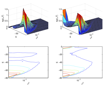
Figure 1: Comparison between the results of one simulation with initial $u=0.15$, called $C2$ (starting from 20 cold clumps of radius $0.4$), and the best fit $f^{(\nu)}$ model ($\nu=0.5$, $\Psi=6.2$). Left set of four panels: Density as measured from the simulation (crosses) vs. the best fit profile (top left). Residuals (in magnitudes) from the $R^{1/4}$ (dotted line) and from the $R^{1/n}$ (with $n=4.46$) law for the best fit projected-density profile (top right). Anisotropy profile of the simulation (crosses) vs. the best fit profile (bottom left). Energy density distribution $N(E)$ (bottom right). Right set of four panels: Final phase space density $N(E,J^{2})$ (left column), compared with that of the best fitting $f^{(\nu)}$ model (right column). The model curve for $N(E)$ and surface for $N(E,J^{2})$ have been computed by a Monte Carlo sampling of phase space.

References

- (1) Bertin, G., Ciotti, L., Del Principe, M. 2002, Astron. Astrophys., 386, 149
- (2) Bertin, G., Stiavelli, M. 1993, Rep. Prog. Phys., 56, 493
- (3) Bertin, G., Trenti, M. 2003, Astrophys. J., 584, 729
- (4) Londrillo, P., Messina, A., Stiavelli, M. 1991, Mon. Not. Roy. Astron. Soc., 250, 54
- (5) Lynden-Bell, D. 1967, Mon. Not. Roy. Astron. Soc., 136, 101
- (6) Stiavelli, M., Bertin, G. 1987, Mon. Not. Roy. Astron. Soc., 229, 61
- (7) Trenti, M., Ph.D. Thesis, Scuola Normale Superiore, Pisa, in preparation
- (8) van Albada, T.S. 1982, Mon. Not. Roy. Astron. Soc., 201, 939