Can long-term periodic variability and jet helicity in 3C 120 be explained by jet precession?

Abstract

Optical variability of 3C 120 is discussed in the framework of jet precession. Specifically, we assume that the observed long-term periodic variability is produced by the emission from an underlying jet with a time-dependent boosting factor driven by precession. The differences in the apparent velocities of the different superluminal components in the milliarcsecond jet can also be explained by the precession model as being related to changes in the viewing angle. The evolution of the jet components has been used to determine the parameters of the precession model, which also reproduce the helical structure seen at large scales. Among the possible mechanisms that could produce jet precession, we consider that 3C 120 harbours a super-massive black hole binary system in its nuclear region and that torques induced by misalignment between the accretion disc and the orbital plane of the secondary black hole are responsible for this precession; we estimated upper and lower limits for the black holes masses and their mean separation.

1 Introduction

3C 120 (z=0.033; Baldwin et al. 1980), also known as II Zw 14 and PKS 0430+052, is usually classified as a Seyfert 1 galaxy, although its morphology in the optical band is not as simple as that of a typical galaxy of this class. Indeed, photometric and spectroscopic studies seem to indicate that 3C 120 either passed, or it is still passing through a merger process (e.g., Soubeyran et al. 1989; Hjorth et al. 1995). The residual I-band image obtained by Hjorth et al. (1995) after subtraction of the stellar contribution, showed a complex structure formed by several condensations, probably associated to active star forming regions (Soubeyran et al., 1989), and an elongated structure which coincides with the kilo-parsec radio jet detected at 5 GHz (Walker, Walker & Benson, 1988). In fact, this large scale jet is the extension of a sub-parsec scale jet, which remains relativistic up to distances of about 100 kpc. (Walker, Benson & Unwin, 1987a).

Several superluminal radio components have been detected in the jet (e.g., Gómez et al. 1998, 2000; Walker et al. 2001; Gómez et al. 2001), with different velocities and position angles, besides a stationary core smaller than 54 $\mu$as (0.025$h^{-1}$ pc) (Gómez, Marscher & Alberdi, 1999). There is also evidence of the existence of trailing shocks in the jet (Gómez et al., 2001), that is, features that do not originate in the jet inlet. These features could be related to pinch-mode jet-body instabilities produced by the propagation of the superluminal components, as shown recently by numerical simulations (e.g., Agudo et al. 2001; Aloy et al. 2003). The observed correlation between dips in the X-ray emission and ejection of superluminal components has been interpreted as a consequence of the connection between jet origin and the accretion disc, such as in the case of microquasars (Marscher et al., 2002).

3C 120 presents variability in all bands and in different time-scales (e.g., Epstein et al. 1972; Halpern 1985; Webb 1990; Shukla & Stoner 1996; Zdziarski & Grandi 2001). The complex variability found in the historical B-band light curve was decomposed by Webb (1990) in three different components: a linear time decrease of its magnitude due to the diminution of the accretion rate, a long-term variability with a period of 12.4-yr produced by thermal or viscous instabilities in the accretion disc, and short-term variations associated to magnetic eruptions in the magnetized disc.

In this paper, the reported 12.4-yr variability is interpreted as periodic boosting of the radiation emitted by the underlying jet, caused by jet precession. This model also explains the differences in superluminal velocities and position angles of the different components, assuming that they represent the direction of the jet inlet at the epoch in which the components were formed. Furthermore, the complex jet structure of 3C 120 at large scales is also studied in the framework of jet precession. Jet precession has been claimed by several authors in order to explain the radio structure of several quasars, BL Lacs and radio-galaxies (e.g., Gower & Hutchings 1982; Gower et al. 1982; Gower & Hutchings 1984; Roos & Meuers 1987; Abraham & Carrara 1998; Abraham & Romero 1999; Abraham 2000; Stirling et al. 2003; Caproni & Abraham 2003), suggesting that jet precession is not so uncommon phenomenon in the Universe. We shall adopt $h=0.7$ and $q_{0}=0.5$ throughout the paper.

2 Jet precession

2.1 Observational evidences

High-resolution observations between 5 and 43 GHz (Walker et al., 1982; Walker, Benson & Unwin, 1987b; Gómez, Marscher & Alberdi, 1999; Gómez et al., 2000; Fomalont et al., 2000; Homan et al., 2001; Walker et al., 2001) give the core-component distance $r$ and the position angle on the plane of sky $\eta$ for each feature in the sub-parsec scale jet. Using data at different epochs, the apparent proper motion $\mu$ is calculated and the apparent velocity $\beta_{\mathrm{app}}$ in units of light speed $c$ is obtained from:

$$\beta_{\mathrm{app}}=\frac{q_{0}z+(q_{0}-1)[(1+2q_{0}z)^{1/2}-1]}{100hq_{0}^{2}(1+z)}\mu$$ (1)

where $h=H_{0}/100$, $H_{0}$ is the Hubble constant in units of km s^-1 Mpc^-1, $q_{0}$ is the deceleration parameter and $z$ is the redshift. The ejection epoch $t_{\mathrm{0}}$ of each component is obtained by back-extrapolation of their linear motions. The kinematic parameters of the different superluminal features are presented in Table 1.

Table 1: Kinematic parameters of the superluminal components of 3C 120.

Component	Literature	$t_{\mathrm{0}}$ (yr)	$\mu$ (mas/yr)	$h\beta_{\mathrm{app}}$	$\eta$ ($\degr$)
K1	-	1976.7 $\pm$ 0.6	3.01 $\pm$ 0.33	4.6 $\pm$ 0.5	-113 $\pm$ 2
K2	-	1977.6 $\pm$ 0.6	3.01 $\pm$ 0.39	4.6 $\pm$ 0.6	-108 $\pm$ 4
K3	A[1]	1978.8 $\pm$ 0.5	2.75 $\pm$ 0.33	4.2 $\pm$ 0.5	-101 $\pm$ 9
K4	B[1]	1980.3 $\pm$ 0.5	3.01 $\pm$ 0.26	4.6 $\pm$ 0.4	-99 $\pm$ 5
K5	C[1]	1981.0 $\pm$ 0.5	2.48 $\pm$ 0.26	3.8 $\pm$ 0.4	-95 $\pm$ 6
K6	D[1]	1981.7 $\pm$ 0.4	2.35 $\pm$ 0.20	3.6 $\pm$ 0.3	-97 $\pm$ 6
K7	E[1]	1982.6 $\pm$ 0.4	2.22 $\pm$ 0.20	3.4 $\pm$ 0.3	-101 $\pm$ 7
K8	F[1]	1983.3 $\pm$ 0.5	2.09 $\pm$ 0.20	3.2 $\pm$ 0.3	-102 $\pm$ 8
K9	G[1]	1984.3 $\pm$ 0.5	2.09 $\pm$ 0.39	3.2 $\pm$ 0.6	-109 $\pm$ 8
K10	H+I[1]	1985.4 $\pm$ 0.8	2.42 $\pm$ 0.39	3.7 $\pm$ 0.6	-119 $\pm$ 5
K11	I[1]	1986.1 $\pm$ 0.6	2.81 $\pm$ 0.33	4.3 $\pm$ 0.5	-120 $\pm$ 6
K12	J[1]	1986.7 $\pm$ 0.6	2.35 $\pm$ 0.33	3.6 $\pm$ 0.5	-120 $\pm$ 7
K13	K[1]	1988.0 $\pm$ 0.4	2.81 $\pm$ 0.39	4.3 $\pm$ 0.6	-117 $\pm$ 7
K14	A[2]	1994.5 $\pm$ 0.7	2.22 $\pm$ 0.26	3.4 $\pm$ 0.4	-108 $\pm$ 3
K15	B[2], K1A/U1A[3]	1994.9 $\pm$ 0.7	2.16 $\pm$ 0.26	3.3 $\pm$ 0.4	-106 $\pm$ 3
K16	C[2], K1B/U1B[3]	1995.2 $\pm$ 0.6	2.09 $\pm$ 0.26	3.2 $\pm$ 0.4	-111 $\pm$ 3
K17	D[2,4], d[2,4]	1995.5 $\pm$ 0.4	2.16 $\pm$ 0.20	3.3 $\pm$ 0.3	-113 $\pm$ 3
K18	G2[2], g[2]	1996.3 $\pm$ 0.5	2.09 $\pm$ 0.26	3.2 $\pm$ 0.4	-119 $\pm$ 5
K19	H[2,4], h[2,5]	1996.8 $\pm$ 0.4	2.09 $\pm$ 0.20	3.2 $\pm$ 0.3	-120 $\pm$ 5
K20	J[2,4], j[2]	1997.0 $\pm$ 0.4	2.16 $\pm$ 0.26	3.3 $\pm$ 0.4	-116 $\pm$ 3
K21	K[2,4], k[5]	1997.3 $\pm$ 0.4	2.22 $\pm$ 0.20	3.4 $\pm$ 0.3	-117 $\pm$ 5
K22	L[2,4], l2[5]	1997.5 $\pm$ 0.4	2.29 $\pm$ 0.20	3.5 $\pm$ 0.3	-124 $\pm$ 4
K23	o1+o2[5]	1998.2 $\pm$ 0.4	2.22 $\pm$ 0.13	3.4 $\pm$ 0.2	-122 $\pm$ 3

We have labelled jet components as ‘K’ followed by a number related to the epoch in which they were formed (‘1’ for the oldest one). We also present the labels given in earlier works in the second column of Table 1. Except for K10, we kept strictly the previous identifications. Considering the uncertainties, the listed parameters are compatible with those found in the literature (e.g., Gómez et al. 1998, 2001; Walker et al. 2001).

We can note in Table 1 that the different jet components were ejected with different velocities and position angles. A possible interpretation for this behaviour is in terms of a precessing jet model: precession changes the orientation of the jet inlet in relation to the line of sight, so that the direction in which the components are ejected, as well as their apparent velocities become a function of time. For the present discussion, it is not relevant whether the jet components are assumed to be plasmons or shocks since we are only interested in the kinematic aspects.

At lower resolution, VLBI observations at 1.7 GHz have revealed that the jet structure of 3C 120 is extremely complex (Walker et al., 2001); it presents sub-structures in scales of tenths of a parsec that move superluminally, a possible stationary component located at an angular distance of about 81 mas from the core and a jet aperture that is larger in the southern direction, specially after about 180 mas, where there is also a decrease in the apparent velocity.

Those characteristics were interpreted by Walker et al. (2001) as an indicative of the presence of a helical pattern in the jet. However, they can also be understood in terms of the precession model that explains the sub-parsec behavior of the superluminal jet.

2.2 Precession model

We will derive the instantaneous appearance of the jet, assuming that it is the result of the combination of plasma elements ejected in different epochs, with different angles in relation to the line of sight. Let us consider a plasma element ejected at time $t_{0}$ with velocity $c\beta$ ($c$ is the light speed) in the comoving reference frame. This element will have a velocity $c\beta_{\mathrm{app}}$ in the observer’s reference frame given by:

$$\beta_{\mathrm{app}}=\frac{\pm\beta\sin[\phi(t_{0})]}{1\pm\beta\cos[\phi(t_{0})]}$$ (2)

where $\phi$ is the angle between the moving direction of the element and the line of sight. The signs ‘+’ and ‘-’ refer to the jet and the counterjet respectively. As the counterjet has not been detected for scales smaller than 100 kpc (Walker, Benson & Unwin, 1987a), we will consider only the jet hereafter.

Due to jet precession, $\phi$ and $\eta$ are functions of time $t$ given by:

$$\phi(t)=\arcsin\biggl{[}{\sqrt{x(t)^{2}+y(t)^{2}}}\biggr{]}$$ (3)

$$\eta(t)=\arctan\biggl{[}\frac{y(t)}{x(t)}\biggr{]}$$ (4)

with

$$x(t)=A(t)\cos\eta_{0}-B(t)\sin\eta_{0}$$ (5)

$$y(t)=A(t)\sin\eta_{0}+B(t)\cos\eta_{0}$$ (6)

and

$$A(t)=\cos\Omega\sin\phi_{0}+\sin\Omega\cos\phi_{0}\sin\omega t$$ (7)

$$B(t)=\sin\Omega\cos\omega t$$ (8)

where $\omega$ is the precession angular velocity, $\Omega$ is the semi-aperture angle of the precession cone, $\phi_{0}$ is the angle between the precession cone axis and the line of sight and $\eta_{0}$ the projected angle of the cone axis on the plane of the sky.

In the determination of the precession parameters, we used all jet components listed in Table 1 as model constraints. As data were obtained at different frequencies, shifts in the core-component distances due to opacity effects may become quantitatively important in the calculation of the proper motions. To perform opacity correction in the observational data, we used the formalism given in Blandford & Königl (1979), which uses the integrated synchrotron luminosity $L_{\mathrm{syn}}$, the ratio between upper and lower limits of the energy distribution in the relativistic jet particles $\Gamma_{\mathrm{max}}/\Gamma_{\mathrm{min}}$, the intrinsic jet aperture angle $\psi^{\prime}$, a constant parameter $k_{\mathrm{e}}$ and the angle $\phi$ between the jet direction and the line of sight. The relation between these quantities is presented in Appendix A.

As in Lobanov (1998), we assumed $k_{\mathrm{e}}=1$, $\Gamma_{\mathrm{max}}/\Gamma_{\mathrm{min}}=100$, $\psi^{\prime}=0.5\degr$ and $L_{\mathrm{syn}}=8.4\times 10^{41}$ erg s^-1. However, in our model, the angle $\phi$ is a function of time and depends on the precession model parameters. Therefore, the corrections were determined iteratively together with the model. The final result was a small correction, with a mean value between 5 and 43 GHz of $\Delta r_{\mathrm{core}}=0.147$ mas, with upper and lower limits of 0.130 and 0.164 mas, respectively.

To find the precession parameters we consider a period of 12.3 yr, almost the same as the long-term variability period found by Webb (1990) in the B-band light curve. In order to determine the best set of model parameters, we chose a $\gamma$ factor compatible with the velocity of the fastest component ($\sim 4.6h^{-1}$ c), given by $\gamma_{min}=(1+\beta_{\mathrm{app}}^{2})^{1/2}$ ($\gamma_{min}\sim 6.7$ for $h=0.7$). After fixing a value for $\gamma$ close to its lower limit, we selected the parameters $\Omega$, $\phi_{\mathrm{0}}$ and $\eta_{\mathrm{0}}$ that fitted the apparent velocities and position angles of the jet components. Then, we checked the behavior of $h\beta_{\mathrm{app}}$ and $\eta$ as functions of time, assuming that the position angle of the jet component represents the jet position at the epoch when the component was formed. This procedure was done iteratively until a good fitting for the data was obtained.

The precession parameters are given in Table 2, while the model fitting in the ($\eta$, $h\beta_{\mathrm{app}}$), ($t$, $h\beta_{\mathrm{app}}$) and ($t$, $\eta$) planes is presented in Fig. 1. It is also possible to fit the data using larger values for $\gamma$ and other jet parameters (decreasing $\Omega$ and $\phi_{\mathrm{0}}$). As a consequence of that, not only the predicted position angles are much larger than those observed in the VLBI maps but also the time variations of the Doppler boosting factor become smaller than those necessary to explain the optical light curve (see Section 4 for further discussion).

Table 2: Parameters of the precession model for the parsec-jet of 3C 120.

$P$ (yr)a	$\gamma$	$\Omega$ ($\degr$)	$\phi_{\mathrm{0}}$ ($\degr$)	$\eta_{\mathrm{0}}$ ($\degr$)
12.3 $\pm$ 0.3	6.8 $\pm$ 0.5	1.5 $\pm$ 0.3	4.8 $\pm$ 0.5	-108 $\pm$ 4

• Measured in the framework fixed at the observer.

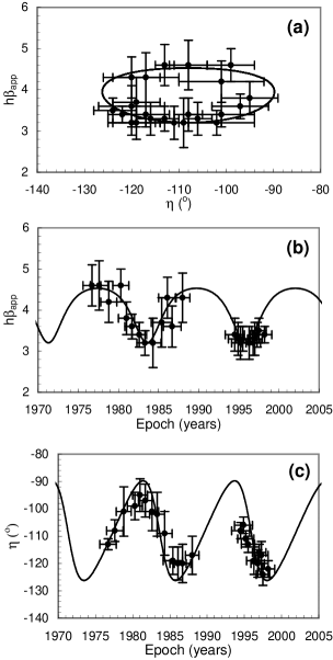
Figure 1: Precession model for 3C 120. The parameters are listed in Table 2. (a) - (c): Solutions of the model on the planes ($\eta$, $\mathrm{h}\beta_{\mathrm{app}}$), ($t$, $\mathrm{h}\beta_{\mathrm{app}}$) and ($t$, $\eta$).

3 Large scale jet structure of 3C 120

Taking into account that even though the jet components have ballistic trajectories on the plane of the sky, a snapshot in time of a precessing jet will show an helicoidal pattern. To compare our results with the large-scale jet structure described by Walker et al. (2001), we calculated the apparent proper motion $\mu$ of a jet element from $c\beta_{\mathrm{app}}[\phi(t)]$ through equation (1).

Using equations (2)-(8), we determined the right ascension and declination offsets of the jet element in relation to the core ($\Delta\alpha$ and $\Delta\delta$ respectively) in a given time $t_{\mathrm{obs}}$ ($t_{\mathrm{obs}}\geq t_{0}$) through:

$$\Delta\alpha(t_{\mathrm{obs}})=\mu_{\alpha}(t_{0})\cdot(t_{\mathrm{obs}}-t_{0})$$ (9)

$$\Delta\delta(t_{\mathrm{obs}})=\mu_{\delta}(t_{0})\cdot(t_{\mathrm{obs}}-t_{0})$$ (10)

where $\mu_{\alpha}$ and $\mu_{\delta}$ are respectively the apparent proper motions in right ascension and declination, being related to $\mu$ and $\eta$ by:

$$\mu_{\alpha}(t_{0})=\mu(t_{0})\cdot\sin[\eta(t_{0})]$$ (11)

$$\mu_{\delta}(t_{0})=\mu(t_{0})\cdot\cos[\eta(t_{0})]$$ (12)

Assuming now a continuous jet and the precession parameters listed in Table 2, we simulated the jet appearance at the five distinct epochs for which 1.7 GHz observations are available (Walker et al., 2001): $t_{\mathrm{obs}}$ = 1982.77, 1984.26, 1989.85, 1994.44 and 1997.70, as shown in Fig. 2. Note that this approach is similar to that used to model the radio structure of several quasars and radio-galaxies in previous papers (Gower & Hutchings, 1982; Gower et al., 1982; Gower & Hutchings, 1984; Roos & Meuers, 1987).

Figure 2: Helicoidal pattern due to jet precession. Each one of the panels corresponds to snapshots of the precession helix in five distinct epochs, chosen as the same epochs of the 1.7 GHz observations (Walker et al., 2001). The big circles superposed upon the helices represent the position of jet components which can be related to the features L2-L9 found by Walker et al. (2001).

Each point of the helices in Fig. 2 corresponds to a given plasma element, although in the case of a continuous jet, the helix driven by precession is continuous. The wavelength of the helices is basically related to the precession period, while the amplitude depends mainly on $\Omega$ and $\phi_{\mathrm{0}}$. As this pattern is not stationary in time, since the precession helix is tied up with the jet movement, the configuration observed in a given time $t$ will be seen again after an interval $\Delta t$, which corresponds to 12.3 yr in the case of 3C 120.

The comparison of the predicted helicoidal patterns in Fig. 2 with the VLBI maps obtained by Walker et al. (2001) show that the observed jet aperture is reasonably well described by jet precession in the inner parts of the jet. The maps reveal also the existence of discrete structures labelled as L2-L9, which could be superluminal. In order to compare these observations with our model, we assumed that L2-L9 were ejected at different epochs and have ballistic motions. We present in Table 3 their kinematic parameters, which are used to calculated their right ascension and declination offsets for the five epochs given in Fig. 2 (their positions are marked by big circles). Components L7 and L8 can be identified respectively as the evolved components K5 and K8 in the parsec-scale jet, as presented in Table 1.

Table 3: Kinematic parameters of the superluminal components observed at 1.7 GHz in the large scale jet of 3C 120.

Component	$t_{\mathrm{0}}$ (yr)	$\mu$ (mas/yr)	$h\beta_{\mathrm{app}}$	$\eta$ ($\degr$)
L2	1921.3	2.24	3.4	-95
L3	1945.0	2.49	3.8	-90
L4	1957.2	2.52	3.9	-90
L5	1966.4	2.94	4.5	-101
L6	1970.2	2.32	3.5	-93
L7	1980.7	2.76	4.2	-91
L8	1983.7	2.10	3.2	-108
L9	1992.1	2.88	4.4	-95

A good agreement between the offsets shown in Fig. 2 and the locations of L2-L9 in the 1.7 GHz maps of 3C 120 is found, suggesting that the simple approach assumed in this work (ballistic motion + precession) provide a reasonable description for their kinematic behaviour in such scales. However, this conclusion could be somehow misleading, since we can rule out neither the possibility that L2-L9 are formed by superposition of several unresolved components in the maps, nor that jet components have non-ballistic trajectories in those scales.

At larger distances from the core ($\mid\Delta\alpha\mid>80$ mas), we see that the full range of position angles provided by our precession model is not found in the observational data, in the sense that the amplitudes of the precession helices towards the southern direction are systematically larger than the observed jet aperture. A possible explanation for this behavior is the existence of an external medium which does not allow the jet propagation in some directions and could lead to the formation of a stationary component, as observed in the VLBI maps at $\Delta\alpha\approx-80$ mas and $\Delta\delta\approx-17$ mas.

From these results, it is reasonable to verify in what conditions the quasi-stationary component could be formed. The interaction between the fluids at different velocities will produce shock waves propagating along the jet. In the case of strong shocks and assuming that the fluid can be described by a relativistic adiabatic equation of state ($p\propto N^{4/3}$, where $p$ is the thermodynamic pressure), the jump condition between the pre-shock and pos-shock regions is (e.g., Blandford & McKee 1976; Romero 1996):

$$\frac{N_{\mathrm{ps}}}{N_{\mathrm{j}}}=4\gamma_{\mathrm{ps}}\gamma\biggl{[}1-\sqrt{1-\gamma_{\mathrm{ps}}^{-2}-\gamma^{-2}+(\gamma_{\mathrm{ps}}\gamma)^{-2}}\biggr{]}+3$$ (13)

where $N_{\mathrm{j}}$ and $\gamma$ are respectively the proper particle density and the bulk Lorentz factor in the pre-shock region, while $N_{\mathrm{ps}}$ and $\gamma_{\mathrm{ps}}$ are the same quantities in the pos-shock region.

If the observed feature is actually stationary, its proper motion must not produce displacements larger than the angular resolution of the maps, otherwise its motion would have been detected during this interval. From the beam-size in right ascension and declination (4 and 12.5 mas respectively) and the interval between the last and first observation ($\sim$14.93 yr), we estimated an upper limit for the apparent proper motion of about 0.27 mas/yr, which results in an apparent velocity smaller than 0.41$c$.

To calculate the true velocity of the quasi-stationary knot, it is necessary to know its viewing angle. However, only its position angle (about $-102\degr$) is known and the precession model allows two different solutions for the viewing angle: 3.3$\degr$ and 6.2$\degr$. Using equation (2) with $\phi=6.2\degr$, we found that the upper limits for the true velocity and the associated Lorentz factor for the quasi-stationary component are respectively $0.80c$ and $1.67$, while for $\phi=3.3\degr$ the same quantities have upper limits of $0.88c$ and $2.11$.

With these limits and assuming that the quasi-stationary component is associated with the pos-shock region, we found from equation (13) that the minimum particle density required to slow down the jet is $12N_{\mathrm{j}}$ and $10N_{\mathrm{j}}$ for the viewing angles $6.2\degr$ and $3.3\degr$, respectively. For an external medium like the clouds of the Narrow Line Region, with typical number density of 10⁴ cm^-3, and for a viewing angle of 6.2$\degr$, we obtain an upper limit of of 833 cm^-3 for the jet density, which is reasonable in terms of ordinary relativistic jets (e.g., Walker, Benson & Unwin 1987a; Altschuler 1989; Romero 1996).

4 The optical boosted emission of the underlying jet

The luminosity of 3C 120 observed in the optical band might be the result of the superposition of thermal contribution from the accretion disc with non-thermal contribution produced, e.g., in the underlying jet and in the superluminal components. If we consider that the underlying jet is represented by a relativistic continuous fluid, its flux density measured in the observer’s reference frame $S_{\mathrm{j}}(\nu)$ is related to that in the comoving frame $S_{\mathrm{j}}^{\prime}(\nu)$ by (Lind & Blandford, 1985):

$$S_{\mathrm{j}}(\nu)=S_{\mathrm{j}}^{\prime}(\nu)\delta(\phi,\gamma)^{2+\alpha}$$ (14)

where $\alpha$ is the spectral index ($S_{\nu}\propto\nu^{-\alpha}$) and $\delta$ is the Doppler factor, defined as:

$$\delta(\phi,\gamma)=[\gamma(1-\beta\cos\phi)]^{-1}$$ (15)

Due to jet precession, $\delta$, and consequently the observed emission from the underlying jet, become time dependent; the closer the jet is to the line of sight, the higher the boosting effect is.

Depending on the intrinsic jet intensity, periodic boosting variations could produce detectable variability in the light curve, as in the case of 3C 279 and OJ 287 (Abraham & Carrara, 1998; Abraham, 2000). To reproduce this light curve and following the suggestion by Webb (1990) of a possible secular linear variation, we modeled the contribution of the underlying jet assuming that its emission is described by equation (14), with $S_{\mathrm{j}}^{\prime}(\nu)$ given by:

$$S_{\mathrm{j}}^{\prime}(\nu,t)=S_{\mathrm{1}}^{\prime}(\nu)+S_{\mathrm{2}}^{\prime}(\nu)\cdot(t-1965)\cdot\frac{\delta(\phi,\gamma)}{(1+z)}$$ (16)

The term $\delta(\phi,\gamma)/(1+z)$ in equation (16) is due to the transformation of the time measured in the comoving frame to the observer’s reference frame. Combining equations (14) and (16), we have:

$$S_{\mathrm{j}}(\nu,t)=\biggl{[}S_{\mathrm{1}}^{\prime}(\nu)+S_{\mathrm{2}}^{\prime}(\nu)\cdot(t-1965)\cdot$$

$$\cdot\frac{\delta(\phi,\gamma)}{(1+z)}\biggr{]}\cdot\delta(\phi,\gamma)^{2+\alpha}$$ (17)

Observations in the B and I bands of the optical counterpart of the kilo-parsec radio jet led to $\alpha_{B-I}=2.0$ (Hjorth et al., 1995); assuming that this value is also valid for the parsec-scale jet and using $\delta$ from the precession model, we simulated the long-term periodic variability in two different cases: Model A, with a secular time decrease of the intrinsic flux density, and Model B, in which the linear term was neglected ($S_{\mathrm{2}}^{\prime}=0$). The model parameters are given in Table 4, where $S_{\mathrm{1}}^{\prime}(\nu)$ was chosen to keep $S_{\mathrm{j}}(\nu,t)$ smaller than the minimum observed value at all epochs. For that reason the values of the parameters should be considered as upper limits.

Table 4: Model parameters used in equation (17) to describe long-term variability in the B-band light curve of 3C 120.

		$S_{\mathrm{1}}^{\prime}$ ($\mu$Jy)		$S_{\mathrm{2}}^{\prime}$ ($n$Jy)
MODEL A		0.19		-0.14
MODEL B		0.16		0.0

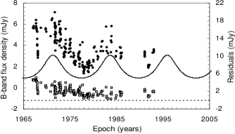
Figure 3: Contribution of the underlying jet for the variability in the B-band light curve of 3C 120 in the case of Model B (see Table 4). The full circles are related to the observed flux density, while open squares are the residuals obtained after subtracting the contribution of the underlying jet (solid lines). The dashed line corresponds to residual equals to zero.

Boosting effects produce a substantial increase in the underlying jet flux density in both models. Since the residuals obtained from the subtraction of the observed flux density from the model predictions are very similar in the two cases, the secular linear decrease in the B-band brightness proposed originally by Webb (1990) seems to be unnecessary, at least after 1965. We show in Fig. 3 the flux density calculated from model B, the B-band historical light curve of 3C 120 and the difference between them.

5 A possible super-massive black hole binary system in the nuclear region of 3C 120

Jet precession can be produced by the Lense-Thirring effect (Lense & Thirring, 1918), in which precession is due to the misalignment between the angular momenta of the accretion disk and of a Kerr black hole. This effect was investigated by Lu (1992) for several AGNs; for all of them, the period found was of the order of thousands of years. Using the same assumptions for the central object in 3C 120, which has a central mass of $3.4\times 10^{7}$ M_☉ (Peterson et al., 1998), we obtain an even longer precession period. On the other hand, jet precession with periods of several years can be produced in super-massive black hole binary systems, when the secondary black hole has an orbit non-coplanar with the primary accretion disc, which induces torques in its inner parts (e.g., Katz 1980, 1997; Romero et al. 2000) Thus, we will assume that the former scenario, in which jet inlet precession is induced in super-massive black hole binary system, is more suitable to 3C 120 and, from this assumption, the binary system parameters will be estimated.

Let us consider that the primary and secondary black holes, with masses $M_{\mathrm{p}}$ and $M_{\mathrm{s}}$ respectively, are separated by a distance $r_{\mathrm{ps}}$. From Kepler’s third law, we can relate $r_{\mathrm{ps}}$ to the orbital period of the secondary around the primary black hole $P_{\mathrm{ps}}$ through:

$$r_{\mathrm{ps}}^{3}=\frac{\mathrm{G}M_{\mathrm{tot}}}{4\pi^{2}}P_{\mathrm{ps}}^{2}$$ (18)

where G is the gravitational constant and $M_{\mathrm{tot}}$ is the sum of the masses of the two black holes.

In the observer’s reference frame, the orbital period $P_{\mathrm{ps}}^{obs}$ is given by:

$$P_{\mathrm{ps}}=\frac{P_{\mathrm{ps}}^{obs}}{(1+z)}$$ (19)

According to Romero et al. (2000), density waves, which disturb the accretion rate and originate the superluminal components, could be produced when the secondary black hole crosses the primary accretion disc. As the secondary crosses the disc twice per orbit, we used $P_{\mathrm{ps}}^{obs}$ as twice the mean separation between the emergence of superluminal components, which leads to $P_{\mathrm{ps}}\approx 1.4$ yr.

Using reverberation mapping techniques, Peterson et al. (1998) estimated a virial mass for the central source of $3.4\times 10^{7}$ M_☉. We assumed that this value corresponds to the total mass of the binary system and from equation (18), with the values of $P_{\mathrm{ps}}$ and $M_{\mathrm{tot}}$ given above, we found that $r_{\mathrm{ps}}\approx 5.9\times 10^{15}$ cm. Considering that the outer radius of the precessing part of the disc is $r_{\mathrm{d}}$, Papaloizou & Terquem (1995) and Larwood (1997) calculated its precession period $P_{\mathrm{d}}$ in terms of the masses of the black holes:

$$\frac{2\pi}{P_{\mathrm{d}}}(1+z)=-\frac{3}{4}\left(\frac{7-2n}{5-n}\right)\frac{GM_{\mathrm{s}}}{r_{\mathrm{ps}}^{3}}\times$$

$$\times\frac{r_{\mathrm{d}}^{2}}{\sqrt{GM_{\mathrm{p}}r_{\mathrm{d}}}}\cos\theta$$ (20)

where $n$ is the politropic index of the gas (e.g., $n=3/2$ and $n=3$ for the non-relativistic and relativistic cases, respectively) and $\theta$ is the angle between the orbit of the secondary and the plane of the disc.

If the jet and accretion disc are coupled, the jet precesses at same rate than the disc ($P=P_{\mathrm{d}})$, forming a precession cone with half-opening angle equal to the angle of orbit inclination ($\Omega=\theta$). Thus, replacing $M_{\mathrm{s}}$ by $M_{\mathrm{tot}}-M_{\mathrm{p}}$ in equation (20), we can calculate $r_{\mathrm{d}}$ in terms of $M_{\mathrm{p}}$ and $M_{\mathrm{tot}}$:

$$r_{\mathrm{d}}=\left[-\frac{8\pi}{3}\left(\frac{5-n}{7-2n}\right)\frac{(1+z)}{P\cos\Omega}\frac{r_{\mathrm{ps}}^{3}}{\sqrt{GM_{\mathrm{tot}}}}\right]^{2/3}\times$$

$$\times\frac{x_{\mathrm{p}}^{1/3}}{\left(1-x_{\mathrm{p}}\right)^{2/3}}$$ (21)

where $x_{\mathrm{p}}=M_{\mathrm{p}}/M_{\mathrm{tot}}$. In Fig. 4, we plot $r_{\mathrm{d}}$ as a function of $x_{\mathrm{p}}$ using the precession parameters listed in Table 2. We can observe that the increase of $r_{\mathrm{d}}$ with $x_{\mathrm{p}}$ is more pronounced after $x_{\mathrm{p}}\approx 0.7$, such that little variations in $x_{\mathrm{p}}$ introduces large changes in $r_{\mathrm{d}}$.

Figure 4: Outer radius of the precessing disc as a function of the fractional mass of the primary black hole (full line). The dashed line indicates the separation between the primary and secondary black holes.

This formalism is valid only if the disc precesses as a rigid-body, implying that $r_{\mathrm{d}}$ must be appreciably smaller than $r_{\mathrm{ps}}$ (Papaloizou & Terquem, 1995). This limit provides an additional constrain to the masses of the black holes. The dashed line in Fig. 4 shows the value of $r_{\mathrm{ps}}$ derived from equation (18). In order to satisfy the hypothesis of rigid-body precession, the allowed solutions are found for values of $r_{\mathrm{d}}$ which lie under the dashed line in Fig. 4. It necessarily means that $x_{\mathrm{p}}<0.88$, so that $M_{\mathrm{p}}<3.0\times 10^{7}M_{\sun}$. As $M_{\mathrm{tot}}=M_{\mathrm{p}}+M_{\mathrm{s}}$, we can also obtain an lower limit for the mass of the secondary, which should be higher than $4.0\times 10^{6}M_{\sun}$. Summarizing, we present in Table 5 the parameters of the black hole binary system calculated in this section.

Table 5: Parameters of a possible black hole binary system in the inner parts of 3C 120.

$P_{\mathrm{ps}}$ (yr)	$r_{\mathrm{ps}}$ (cm)	$M_{\mathrm{p}}$ (M☉)a	$M_{\mathrm{s}}$ (M☉)b	$M_{\mathrm{tot}}$ (M☉)c
1.4	$5.9\times 10^{15}$	$3.0\times 10^{7}$	$4.0\times 10^{6}$	$3.4\times 10^{7}$

• Upper limit;

• Lower limit;

• Peterson et al. (1998).

6 Conclusions

Based on the periodicity in the historical B-band light curve and variable jet structure, we propose the existence of jet precession in 3C 120, with a period of 12.3 yr.

We assume that the different apparent velocities of the superluminal components measured at milliarcsecond and larger scales are related to changes in the angle between the jet inlet and the line of sight due to precession, although the superposition of unresolved components and/or interaction with the environment could are acting at the largest scales.

We show that the periodicity in the optical light curve can be produced by the boosted underlying jet, with a time-dependent boosting factor driven by precession. An upper limit of 0.16 $\mu$Jy was estimated for the flux density of the underlying jet in the comoving reference frame. The inclusion of a secular linear term in the analysis of the long-term variability, as in Webb (1990), is not necessary to obtain a good fitting to the light curve.

The helicoidal jet pattern found by Walker et al. (2001) is interpreted in this work also as the result of jet precession. The helix generated by precession reproduces quite well the jet aperture seen in the 1.7-GHz maps up to distances from the core smaller than $\sim$80 mas, where there is a probable stationary component. Beyond that, the helix amplitude is systematically larger in the southern direction, suggesting the existence of an external medium that does not allow jet propagation. In order to produce a stationary component, considering a one-dimensional adiabatic relativistic jet as well as energy and particle flux conservation, we estimate a lower limit of $\sim$12 for the ratio between jet and environment densities.

Assuming that jet precession in 3C 120 is driven by a secondary super-massive black hole in a non-coplanar orbit around the primary accretion disc, using the total mass of the two black holes derived from reverberation mapping techniques and an orbital period of approximately 1.4 yr, we estimate an upper limit of $3.0\times 10^{7}$ M_☉ for the primary black hole mass, a lower limit of $4.0\times 10^{6}$ M_☉ for the secondary mass and a separation between them of about $5.9\times 10^{15}$ cm.

Appendix A Opacity effects on core-component distance and precession jet

As it was pointed out previously (e.g., Blandford & Königl 1979; Lobanov 1996, 1998), the absolute core position $r_{\mathrm{core}}$ depends inversely on the frequency when the core is optically thick, what introduces a shift in the core-component separation. Following Blandford & Königl (1979), we can write the absolute core position as:

$$r_{\mathrm{core}}(\nu)=\frac{4.56\times 10^{-12}(1+z)}{D_{\mathrm{L}}\gamma^{2}k_{\mathrm{e}}^{1/3}\psi\sin\phi}\cdot$$

$$\cdot\left[\frac{L_{\mathrm{syn}}\sin\phi}{\beta(1-\beta\cos\phi)\ln(\Gamma_{\mathrm{max}}/\Gamma_{\mathrm{min}})}\right]^{2/3}\nu^{-1}(\mathrm{mas})$$ (22)

where $z$ is the redshift, $D_{\mathrm{L}}$ is the luminosity distance (in units of parsec), $k_{\mathrm{e}}$ is a constant ($k_{\mathrm{e}}\leq 1$; Blandford & Königl 1979), $L_{\mathrm{syn}}$ is the integrated synchrotron luminosity (in units of erg s^-1), while $\Gamma_{\mathrm{max}}$ and $\Gamma_{\mathrm{min}}$ are related respectively to the upper and lower limits of the energy distribution of the relativistic jet particles. The quantities $\psi$ and $\nu$ are respectively the observed aperture angle of the jet (in radians) and the frequency (in Hz); the former is related to the intrinsic jet aperture angle $\psi^{\prime}$ through (e.g., Mutel et al. 1990):

$$\tan(\psi/2)=\tan(\psi^{\prime}/2)\cot\phi$$ (23)

The core position shift $\Delta r_{\mathrm{core}}$ between frequencies $\nu_{1}$ and $\nu_{2}$ ($\nu_{2}\geq\nu_{1}$) is given by:

$$\Delta r_{\mathrm{core}}(\nu_{1},\nu_{2})=\frac{4.56\times 10^{-12}(1+z)}{D_{\mathrm{L}}\gamma^{2}k_{\mathrm{e}}^{1/3}\psi\sin\phi}\cdot$$

$$\cdot\left[\frac{L_{\mathrm{syn}}\sin\phi}{\beta(1-\beta\cos\phi)\ln(\Gamma_{\mathrm{max}}/\Gamma_{\mathrm{min}})}\right]^{2/3}\frac{(\nu_{2}-\nu_{1})}{\nu_{1}\nu_{2}}(\mathrm{mas})$$ (24)

Note that if we substitute in equation (A3) a simpler version of equation (A2), $\psi\approx\psi^{\prime}\csc\theta$, we obtain equation (11) given in Lobanov (1998).

We can see that equation (A3) depends on the angle between the jet and line of sight; in the case of a jet which is precessing, this angle is a function of time, what obviously introduces a time dependency in $\Delta r_{\mathrm{core}}$. On the other hand, the shifts in the core-component separations do not occur in a fixed direction, but they are oriented according to the direction whose jet inlet is pointed. As the jet inlet is not resolved by observations, changes in its direction will reflect on changes in the position angle of the core region. Thus, a jet component, located at a distance $r$ from the core and with a position angle $\eta$, will have right ascension and declination offsets ($\Delta\alpha$ and $\Delta\delta$ respectively) given by:

$$\Delta\alpha(\nu_{1},\nu_{2})=r(\nu_{1})\sin[\eta(t_{\mathrm{obs}})]-$$

$$-\Delta r_{\mathrm{core}}(\nu_{1},\nu_{2})\sin[\eta_{\mathrm{c}}(t_{\mathrm{obs}})]$$ (25)

$$\Delta\delta(\nu_{1},\nu_{2})=r(\nu_{1})\cos[\eta(t_{\mathrm{obs}})]-$$

$$-\Delta r_{\mathrm{core}}(\nu_{1},\nu_{2})\cos[\eta_{\mathrm{c}}(t_{\mathrm{obs}})]$$ (26)

where $\eta_{\mathrm{c}}$ is the position angle of the core in the epoch $t_{\mathrm{obs}}$ in which observation is acquired. Known the precession model parameters, we are able to determine the second term of the equations (A4a) and (A4b) and correct the component position by core opacity effects; using them, we can determine the corrected core-component distance $r_{\mathrm{corr}}$ through:

$$r_{\mathrm{corr}}(\nu_{1})=[r(\nu_{1})^{2}+\Delta r_{\mathrm{core}}(\nu_{1},\nu_{2})^{2}-$$

$$-2r(\nu_{1})\Delta r_{\mathrm{core}}(\nu_{1},\nu_{2})\cos(\eta-\eta_{\mathrm{c}})]^{1/2}$$ (27)

Note that if $\Delta r_{\mathrm{core}}=0$, $r_{\mathrm{corr}}=r$. Other particular case is found when there is alignment between the position angles of the core and of the jet component ($\eta=\eta_{\mathrm{c}}$), such that $r_{\mathrm{corr}}=r-\Delta r_{\mathrm{core}}$.

Appendix B Glossary

In order to facilitate the reading of the manuscript, we define all the symbols that appear in the text in Table B1.

Table 6: Definition of the symbols used in the text.

Symbol	Meaning
$G$	gravitational constant
$c$	light speed
$H_{0}$	Hubble constant
$h$	$H_{0}/100$
$q_{0}$	deceleration parameter
$z$	redshift
$D_{\mathrm{L}}$	luminosity distance
$r$	core-component distance
$\Delta\alpha$	right ascension offset of components relative to the core position
$\Delta\delta$	declination offset of components relative to the core position
$t_{\mathrm{0}}$	ejection epoch for the jet components
$\eta$	position angle on the plane of the sky of jet components
$\mu$	apparent proper motion of jet components
$\beta_{\mathrm{app}}$	apparent velocity of jet components
$\phi$	viewing angle of jet components
$\omega$	jet precession angular velocity
$P$	jet precession period
$\Omega$	semi-aperture angle of the precession cone
$\phi_{\mathrm{0}}$	angle between the precession cone axis and the line of sight
$\eta_{\mathrm{0}}$	projected angle of the precession cone axis on the plane of the sky
$\beta$	jet bulk velocity
$\gamma$	Lorentz factor of the jet bulk motion
$\delta$	Doppler factor of jet components
$\gamma_{\mathrm{min}}$	lower limit for the jet bulk motion
$\gamma_{\mathrm{ps}}$	Bulk Lorentz factor of the pos-shock region
$p$	thermodynamic pressure
$N_{\mathrm{j}}$	proper particle density of the jet
$N_{\mathrm{ps}}$	proper particle density of the pos-shock region
$n$	politropic index of the gas
$\nu$	frequency
$S_{\mathrm{j}}$	flux density of the underlying jet in the observer’s reference frame
$S_{\mathrm{j}}^{\prime}$	flux density of the underlying jet in the comoving reference frame
$\alpha$	flux density spectral index
$M_{\mathrm{p}}$	mass of the primary black hole
$M_{\mathrm{s}}$	mass of the secondary black hole
$M_{\mathrm{tot}}$	total mass inside the nuclear region
$x_{\mathrm{p}}$	ratio between the primary and the total masses
$r_{\mathrm{ps}}$	separation between the primary and secondary black holes
$P_{\mathrm{ps}}^{obs}$	orbital period of the secondary around the primary black hole in the observer’s reference frame
$P_{\mathrm{ps}}$	orbital period of the secondary around the primary black hole in the source’s reference frame
$r_{\mathrm{d}}$	outer radius of the precessing part of the primary accretion disc
$P_{\mathrm{d}}$	precession period of the accretion disk
$\theta$	angle between the orbital plane of the secondary and the plane of the primary disc
$L_{\mathrm{syn}}$	integrated synchrotron luminosity
$\Gamma_{\mathrm{max}}$	upper limit for the energy distribution of relativistic jet particles
$\Gamma_{\mathrm{min}}$	lower limit for the energy distribution of relativistic jet particles
$\psi^{\prime}$	intrinsic jet aperture angle
$\psi$	observed jet aperture angle
$k_{\mathrm{e}}$	constant parameter
$\Delta r_{\mathrm{core}}$	angular shift in core position
$\eta_{\mathrm{c}}$	core position angle

References

- Abraham & Carrara (1998) Abraham, Z., Carrara, E. A. 1998, ApJ, 496, 172.
- Abraham & Romero (1999) Abraham, Z., Romero, G. E. 1999, A&A, 344, 61.
- Abraham (2000) Abraham, Z. 2000, A&A, 355, 915.
- Agudo et al. (2001) Agudo, I., Gómez, J. L., Martí, J. M., et al. 2001, ApJ, 549, L183.
- Aloy et al. (2003) Aloy, M. Á., Martí, J. M., Gómez, J. L., et al. 2003, ApJ, 585, L109.
- Altschuler (1989) Altschuler, D. R. 1989, Fundam. Cosmic Phys., 14, 37.
- Baldwin et al. (1980) Baldwin, J. A., Carswell, R. F., Wampler, E. J., et al. 1980, ApJ, 236, 388.
- Begelman et al. (1984) Begelman, M. C., Blandford, R. D., Rees, M. J. 1984, Rev. Mod. Phys., 56, 255.
- Blandford & Königl (1979) Blandford, R. D., Königl, A. 1979, ApJ, 232, 34.
- Blandford & McKee (1976) Blandford, R. D., McKee, C. F. 1976, Phys. Fluids, 19, 1130.
- Caproni & Abraham (2003) Caproni, A., Abraham, Z. 2003, ApJ, in press.
- Epstein et al. (1972) Epstein, E. E., Fogarty, W. G., Hackney, K. R., et al. 1972, ApJ, 178, L51.
- Fomalont et al. (2000) Fomalont, E. B., Frey, S., Paragi, Z., et al. 2000, ApJS, 131, 95.
- Gómez et al. (1998) Gómez, J. L., Marscher, A. P., Alberdi, A., Martí, J. M., Ibáñez, J. M. 1999, ApJ, 499, 221.
- Gómez, Marscher & Alberdi (1999) Gómez, J. L., Marscher, A. P., Alberdi, A. 1999, ApJ, 521, L29.
- Gómez et al. (2000) Gómez, J. L., Marscher, A. P., Alberdi, A., Jorstad, S. G., García-Miró, C. 2000, Science, 289, 2317.
- Gómez et al. (2001) Gómez, J. L., Marscher, A. P., Alberdi, A., Jorstad, S. G., Agudo, I. 2001, ApJ, 561, L161.
- Gower & Hutchings (1982) Gower, A. C., Hutchings, J. B. 1982, ApJ, 258, L63.
- Gower et al. (1982) Gower, A. C., Gregory, P. C., Hutchings, J. B., Unruh, W. G. 1982, ApJ, 262, 478.
- Gower & Hutchings (1984) Gower, A. C., Hutchings, J. B. 1984, PASP, 96, 19.
- Halpern (1985) Halpern, J. P. 1985, ApJ, 290, 130.
- Hjorth et al. (1995) Hjorth, J., Vestergaard, M., Sorensen, N., Grundahl, F. 1995, ApJ, 452, L17.
- Homan et al. (2001) Homan, D. C., Ojha, R., Wardle, J. F. C., et al. 2001, ApJ, 549, 840.
- Katz (1980) Katz, J. I. 1980, ApJ, 236, L127.
- Katz (1997) Katz, J. I. 1997, ApJ, 478, 527.
- Larwood (1997) Larwood, J. D. 1997, MNRAS, 290, 490.
- Lense & Thirring (1918) Lense, J., Thirring, H. 1918, Phys. Z., 19, 156.
- Lind & Blandford (1985) Lind, K. R., Blandford, R. D. 1985, ApJ, 295, 358.
- Lobanov (1996) Lobanov, A. P. 1996, in Physics of the Parsec-Scale Structure in the Quasar 3C 345, (NMIMT, Socorro, USA: Ph.D. thesis).
- Lobanov (1998) Lobanov, A. P. 1998, A&A, 330, 79.
- Lu (1992) Lu, Ju-fu. 1992, Chin. Astron. Astrophys., 16/2, 133.
- Marscher et al. (2002) Marscher, A. P., Jorstad, S. G., Gómez, J. L., et al. 2002, Nature, 417, 625.
- Mutel et al. (1990) Mutel, R. L., Phillips, R. B., Su, B., Bucciferro, R. R. 1990, ApJ, 352, 81.
- Papaloizou & Terquem (1995) Papaloizou, J. C. B., Terquem, C., 1995, MNRAS, 274, 987.
- Peterson et al. (1998) Peterson, B. M., Wanders, I., Bertram, R., et al. 1998, ApJ, 501, 82.
- Romero (1996) Romero, G. E. 1996, A&A, 313, 759.
- Romero et al. (2000) Romero, G. E., Chajet, L., Abraham, Z., Fan, J. H. 2000, A&A, 360, 57.
- Roos & Meuers (1987) Roos, N., Meuers, E. J. A. 1987, A&A, 181, 14.
- Shukla & Stoner (1996) Shukla, H., Stoner, R. E. 1996, ApJS, 106, 41.
- Soubeyran et al. (1989) Soubeyran, A., Wlérick, G., Bijaoui, A., et al. 1989, A&A, 222, 27.
- Stirling et al. (2003) Stirling, A. M., Cawthorne, T. V., Stevens, J. A., et al. 2003, MNRAS, 341, 405.
- Walker et al. (1982) Walker, R. C., Seielstad, G. A., Simon, R. S., et al. 1982, ApJ, 257, 56.
- Walker, Benson & Unwin (1987a) Walker, R. C., Benson, J. M., Unwin, S. C. 1987a, ApJ, 316, 546.
- Walker, Benson & Unwin (1987b) Walker, R. C., Benson, J. M., Unwin, S. C. 1987b, in Superluminal Radio Sources, ed. J. A. Zensus & T. J. Pearson (Cambridge: Cambridge Univ. Press), 48.
- Walker, Walker & Benson (1988) Walker, R. C., Walker, M. A., Benson, J. M. 1988, ApJ, 335, 668.
- Walker et al. (2001) Walker, R. C., Benson, J. M., Unwin, S. C., et al. 2001, ApJ, 556, 756.
- Webb (1990) Webb, J. R. 1990, AJ, 99, 49
- Zdziarski & Grandi (2001) Zdziarski, A. A., Grandi, P. 2001, ApJ, 551, 186.