The expected abundance of Lyman-$\alpha$ emitting primeval galaxies.
I. General model predictions.

We present model calculations for the expected surface density of Ly-$\alpha$ emitting primeval galaxies (PGs) at high redshifts. We assume that elliptical galaxies and bulges of spiral galaxies (= spheroids) formed early in the universe and that the Ly-$\alpha$ emitting PGs are these spheroids during their first burst of star formation at high redshift. One of the main assumptions of the models is that the Ly-$\alpha$ bright phase of this first starburst in the spheroids is confined to a short period after its onset due to rapid formation of dust. The models do not only explain the failure of early surveys for Ly-$\alpha$ emitting PGs but are also consistent with the limits of new surveys (e.g. the Calar Alto Deep Imaging Survey - CADIS). At faint detection limits $S_{\mbox{lim}}\leq 10^{-20}$W/m² the surface density of Ly-$\alpha$ emitters is expected to vary only weakly in the redshift range between $z=3$ and $z=6$ with values $>10^{3}/\mbox{deg}^{2}/\Delta z=0.1$ reaching its maximum at $z_{0}\approx 4$. At shallower detection limits, $S_{\mbox{lim}}\geq 3\times 10^{-20}$W/m² the surface density of high-z Ly-$\alpha$ emitters is expected to be a steep function of redshift and detection limit. This explains the low success in finding bright Ly-$\alpha$ galaxies at $z>5$. We demonstrate how the observed surface densities of Ly-$\alpha$ emitting PGs derived from recent surveys constrain the parameters of our models. Finally, we discuss the possibility that two Ly-$\alpha$ bright phases occur in the formation process of galaxies: An initial – primeval – phase in which dust is virtually non-existant, and a later secondary phase in which strong galactic winds as observed in some Lyman break galaxies facilitate the escape of Ly-$\alpha$ photons after dust has already been formed.

1 Introduction

The detection of the ancestors of large present day galaxies (like our Milky Way) during their first phase of violent star formation is currently one of the great challenges for observational cosmology. Commonly, these objects are referred to as primeval galaxies (PGs). Finding them in substantial numbers and over a sufficiently broad range of luminosities would provide us with direct insight into the epoch of galaxy formation in the young universe. Since current wisdom places the PG phase of our Galaxy between redshifts $z=5$ and $z=10$ one should ultimately aim to establish the luminosity function of primeval galaxies and their evolution at several redshifts within this range.

It was not long ago that such observational program would have seemed audacious. But with half a dozen telescopes of the 8-10m class in operation, the detection of star formation rates of ten M_☉/year appears feasible even at $z>5$. Indeed, the last few years have witnessed an enormous progress in identifying young galaxies at very high redshifts (see Dey et al., Dey98 (1998), Weymann et al.  Weymann98 (1998), Hu et al.  Hu98 (1998), Hu99 (1999), Hu02 (2002), Hu03 (2003), Rhoads et al.  Rhoads03 (2003)).

Various techniques have been used to search for galaxies at high redshifts. Currently the most successful method, introduced by Steidel et al. (Steidel92 (1992), Steidel93 (1993), 1996a , 1996b , 1998a , 1998b ) uses the Lyman break and the flat spectral energy distribution blue-wards of the Lyman break as a signature of very distant, young star-forming galaxies. Hundreds of galaxies found in this way have been spectroscopically confirmed to be young star forming galaxies at redshifts $z\simeq 3$ (Steidel et al.  1996a ). In addition several dozens of them could be detected at $z\simeq 4$ (Steidel et al. Steidel99 (1999)). The number density and clustering properties of these Lyman break galaxies are consistent with them being the central galaxies of the most massive dark matter halos present at $z\sim 3$ (Mo et al. Mo99 (1999)). Although the Lyman break galaxies seem to be relatively young star forming galaxies, they cannot represent the population of primeval galaxies in the sense defined above: The strong metal absorption lines in their spectra indicate that their current star formation period must have been preceded by an earlier star burst. The massive stars formed have already substantially enriched the interstellar medium in these systems. Moreover, both the UV continuum slope and the Balmer lines (Pettini et al.Pettini98 (1998)) suggest that the Lyman-break galaxies already contain significant amounts of dust. Therefore, it is now widely accepted that the star forming rates inferred from the UV continua of Lyman-break galaxies have to be corrected upwards by a factor of 2 to 5. The presence of dust also explains why only about 1/3 of the Lyman-break galaxies exhibit a strong Ly-$\alpha$ line: In typical star forming regions every Ly-$\alpha$ photon emitted by the hot OB stars will undergo dozens of multiple resonant scatterings before leaving the region towards the observer. Thus even small amounts of dust could quench the escaping Ly-$\alpha$ emission considerably.

In contrast to the Lyman-break galaxies, all galaxies known at $z>5$ exhibit a very strong Ly-$\alpha$ emission line (rest frame equivalent widths $>5$  nm). This is exactly the spectral signature we expect for the first few hundred million years after the onset of a violent burst of massive star formation and before the newly produced metals could be recycled into the cold phase of the inter-stellar medium. Note that at $z=3$ there still exists a large population of Ly-$\alpha$ bright galaxies (Shapley et al. Shapley03 (2003), Kudritzki et al.  Kudritzki00 (2000)) but their low star forming rates indicate that they represent a population of smaller galaxies in which the ”trigger density” has been reached later than in the Lyman-break systems. The weak continua of Ly-$\alpha$ bright galaxies make them hard to find by color-break techniques, but the strong emission lines should easily be detected in narrow-band searches for emission line objects.

Although early attempts to detect Ly-$\alpha$ bright galaxies at $z\ga 3$ failed (Pritchet Pritchet94 (1994)), we have witnessed a breakthrough in finding these objects at redshifts between 3 and 5 as sufficiently deep detection limits (line fluxes of a few $\times 10^{-20}$ Wm^-2 ) have been reached routinely in the last years (Hu et al. Hu98 (1998),Hu99 (1999),Hu02 (2002), Rhoads et al. Rhoads03 (2003), Maier et al. Maier02 (2003)). The most distant known object in the universe has been found in this way (Hu et al. Hu02 (2002)). But still, the number of Ly-$\alpha$ bright galaxies at $z>5$ which have been found in systematic surveys is very limited, and larger samples are required to draw any firm conclusions about the epoch of galaxy formation.

For both the interpretation of the results of present narrow-band searches for Ly-$\alpha$ bright galaxies and the optimum design of future surveys, it is essential to estimate the expected abundance of these objects under reasonable assumptions about the cosmological parameters and the history of galaxy formation.

Here we present a phenomenological model to predict the expected surface density of Ly-$\alpha$ bright PGs at high redshifts based on ideas which have already been sketched in Thommes & Meisenheimer (Thommes95 (1995)) and Thommes (Thommes96 (1996)).

In principle, the prediction of the abundance of Ly-$\alpha$ bright galaxies at high redshifts can be obtained in two ways: One way starts from a primeval density field in the early universe and follows the collapse of dark matter haloes by N-body simulations or with the Press Schechter formalism. Adding in baryonic matter and a reasonable star formation scenario in combination with a treatment of dust formation and distribution could then predict the abundance of star forming haloes and their star formation rate which – under the assumption of an initial mass function (IMF) – could be converted into a prediction of the number density of Ly-$\alpha$ bright galaxies above a certain detection limit. Haiman and Spaans (Haiman99 (1999)) present calculations along this line. However, it is not trivial to scale such an ab initio approach to the observed abundance of galaxies in the local universe.

Therefore, we pursue the second way in which one tries to extrapolate the local luminosity function of galaxies and their stellar content back into the past. This way has been pioneered by Meier (Meier76 (1976)) and further explored by Baron & White (Baron87 (1987)) leading to predicted surface densities of Ly-$\alpha$ bright PGs at $z\simeq 5$ between 1.4 PGs$/\squareforqed\arcmin/(\Delta z=1)$ (for $q_{0}=0.5$) and 0.05 PGs$/\squareforqed\arcmin/(\Delta z=1)$ ($q_{0}=0.0$) for a survey limit $S_{lim}\geq 10^{-19}$ Wm^-2. Such a high abundance has been clearly ruled out by the narrow-band surveys carried out by Thompson et al. (1995a ) and more recently by Hu et al. (Hu98 (1998)). This has triggered several new efforts to search wider fields to deeper limits (e.g. the Calar Alto Deep Imaging Survey – CADIS see Meisenheimer et al. Meisenheimer97 (1997), Meisenheimer98 (1998), the Large Angle Lyman Alpha survey – LALA, see Rhoads et al. Rhoads00 (2000)). We have identified two main points which Baron & White (Baron87 (1987)) did not take into account: (1) The Ly-$\alpha$ bright phase of PGs might be rather short due to rapid dust formation, and (2) galaxies show a substantial age spread and therefore did not form or start simultaneously with their first star formation. As we will see, both points tend to reduce the expected number densities so that the apparent contradiction between observations and predictions disappears.

In the present paper we will describe the basic assumptions of our models and discuss how choices of the cosmological parameters and the history of galaxy formation and of primeval star formation would influence the observable number density for a very broad range of search redshifts $3<z<13$ and detection limits between $10^{-19}$ and $10^{-21}$  Wm^-2. In a forthcoming paper (Meisenheimer, Thommes and Maier 2004, in the following referred to as paper II) we will try to combine all available survey results to constrain the free model parameters even further and thus provide a much more confined set of predictions which could be used as bench mark for future surveys.

The present paper is structured in the following way: In section 2 we briefly describe the narrow-band imaging technique for detecting Ly-$\alpha$ bright galaxies. In section 3 we describe the principle assumptions, parameters and functions of our model. In section 4 we give a very simplified and transparent version of our model and demonstrate why the earlier predictions by Baron & White (Baron87 (1987)) were much too optimistic. Section 5 explores the full range of model parameters in order to identify those which will most critically affect the predicted number density of Ly-$\alpha$ bright primeval galaxies. In section 6, we summarize the generic results of our model. Section 7 discusses how our results are useful in designing optimum surveys and gives a first account of how well the model agrees with the results of present surveys. This issue will be detailed in the subsequent paper II, in which we will adjust the free model parameters as close as possible to the results of all available emission line surveys. This will constrain the range of free parameters even further.

2 Narrow band imaging technique to search for high-redshift Ly-$\alpha$ galaxies

Any emission line survey must aim to map the three-dimensional phase space of objects $(\alpha,\leavevmode\nobreak\ \delta,\leavevmode\nobreak\ \lambda_{obs})$, where $\alpha,\leavevmode\nobreak\ \delta$ are the positions on the sky and $\lambda_{obs}=(1+z)\lambda_{el}$ is the observed wavelength of the emission line, onto the two-dimensional detector in an optimum way ($\lambda_{el}$= restframe wavelength of the emission line). Standard observational techniques for emission line surveys are reviewed by Pritchet (Pritchet94 (1994)).

We concentrate on the narrow-band imaging technique (see e.g. Hippelein et al. Hippelein03 (2003), Maier et al. Maier02 (2003), Meisenheimer et al. Meisenheimer97 (1997)): Here a rather narrow wavelength range $\Delta\lambda$ is selected by using a narrow-band filter or an imaging Fabry-Perot-Interferometer, while $(\alpha,\leavevmode\nobreak\ \delta)$ is directly mapped onto the detector coordinates $(x,y)$. This technique provides two main advantages for the search of Ly-$\alpha$ galaxies at $z\geq 5$: (a) Since the entire field of view $\Delta\omega$ is mapped onto the detector, two-dimensional methods can be used for background determination and source extraction. In general, they perform much better than the one-dimensional methods used in analyzing long-slit spectra. (b) One can place $\delta\lambda_{n}$ such that it falls into wavelength regimes of low and smooth night sky emission. This is of high importance when searching for Ly-$\alpha$ emission at $z>4.9$ where about 75% of the wavelength range is made rather useless by strong OH-lines in the night sky.

For the following model predictions of the abundance of Ly-$\alpha$ galaxies we assume $\Delta z=\Delta\lambda/\lambda_{Ly\alpha}=0.1$ ($\lambda_{Ly\alpha}$=121.57 nm) which is typical for the narrow-band technique. Three redshift intervals are selected such that the Ly-$\alpha$ line falls into the best night sky windows around $\lambda\simeq 705,\leavevmode\nobreak\ 815,$ and 920 nm (that is $z\simeq 4.8,$ 5.7, and 6.6). In addition, we present predictions for $z=3.5$ ($\lambda=530$ nm, V band), $z=9.3$ ($\lambda=1250$ nm, J band), and $z=12.6$ ($\lambda=1650$ nm, H band).

3 The basic formalism

We want to calculate the surface number density of Ly-$\alpha$ emitting PGs on the sky per solid angle $\Delta\omega$ which have detectable Ly-$\alpha$ fluxes greater than a certain flux limit $S_{lim}$ and which have redshifts $z_{0}$ in an interval $[z_{0}-\Delta z/2,z_{0}+\Delta z/2]$. In a narrow band search for Ly-$\alpha$ emitting objects, $z_{0}$ is given by the central wavelength $\lambda_{0}$ of the narrow band filter and $\Delta z$ by the band width of the filter $\Delta\lambda$ ($\Delta z=\Delta\lambda/\lambda_{Ly\alpha}$ ; $\lambda_{Ly\alpha}$=121.57 nm). Here $\Delta\omega$ refers to the area on the sky which is covered by the entire survey. $\Delta\omega$, $\Delta z$ and $z_{0}$ define a certain comoving volume $\Delta V_{c}$ of the universe. The intrinsic Ly-$\alpha$ flux of PGs at $z_{0}$ which produce observable fluxes of $S_{lim}$ is given by

$$L_{min}(z_{0})\,\,=\,\,4\pi\,S_{lim}\,d_{L}(z_{0})^{2}\,$$ (1)

with the luminosity distance $d_{L}(z_{0})$. We have to calculate the number of PGs in the volume $\Delta V_{c}$ with $L_{Ly\alpha}\geq L_{min}(z_{0})$ at the epoch $t_{0}=t(z_{0})$. This number depends on:

• The galaxy formation history, which determines the number of galaxies in the volume $\Delta V_{c}$ which are just in the process of forming and therefore might be in their Ly-$\alpha$ bright phase at the redshift $z_{0}$.

• The evolution of the Ly-$\alpha$ luminosity of the PGs as a function of time and mass of the PG.

We assume that the stars in ellipticals and bulges (both called spheroids) precede the formation of stars in disks which form out of gas which accretes around the spheroids. Our hypothesis is that most Ly-$\alpha$ emitting PGs will be these spheroids during their first burst of star formation at high redshift (but also refer to our discussion in section 7.4). We assume that such a “proto-spheroid” starts to shine in Ly-$\alpha$ as soon as the first star formation sets in and that the Ly-$\alpha$ luminosity is proportional to the star formation rate (SFR) as long as dust absorption is negligible. Furthermore, it is reasonable to assume that the SFR of the first star burst is proportional to the baryonic mass of the PG. Thus, the Ly-$\alpha$ luminosity of a PG should be proportional to its baryonic mass which we assume to be proportional to the total mass of the dark matter halo surrounding the spheroid. If the SFR is not constant but changes with time, so too does the Ly-$\alpha$ luminosity. However, after some time other effects like dust absorption may quench the Ly-$\alpha$ luminosity of the PGs, so the proportionality to the SFR is no longer valid. We describe this time dependence of the Ly-$\alpha$ luminosity with a function $f(t-t_{s})$ where $t_{s}$ is the epoch at which the galaxy starts to shine in Ly-$\alpha$ (see Fig. 1, we call $t_{s}$ the ignition time):

$$\begin{array}[]{c}L_{Ly_{\alpha}}^{(M_{b})}(t-t_{s})=k_{Ly\alpha}\leavevmode\nobreak\ M_{b}\leavevmode\nobreak\ f(t-t_{s})\\ \\ \mbox{with}\quad f(t-t_{s})\leavevmode\nobreak\ \left\{\begin{array}[]{cc}\equiv 0&\mbox{if $t<t_{s}$}\\ >0&\mbox{if $t>t_{s}$}\end{array}\right.\end{array}$$ (2)

$k_{Ly\alpha}$ gives the factor of proportionality between SFR and Ly-$\alpha$ flux in a dust-free medium. $M_{b}$ denotes the baryonic mass of the PG which we assume to be proportional to the total mass $M$ of the PG. $L_{Ly_{\alpha}}^{(M_{b})}(t-t_{s})$ gives the Ly-$\alpha$ luminosity of a galaxy with mass $M_{b}$ at the epoch $t$ (time since the big bang), which started to shine in Ly-$\alpha$ at the epoch $t_{s}$. Because of the assumed proportionality between the Ly-$\alpha$ flux and the PG mass $M$, there exists a lower limit $M_{min}$ for the PGs observed at redshift $z_{0}$, which can get luminous enough in Ly-$\alpha$ that they have an observable flux $>S_{lim}$. PGs with $M<M_{min}$ remain always too faint in Ly-$\alpha$ to be detectable above the survey flux limit $S_{lim}$.

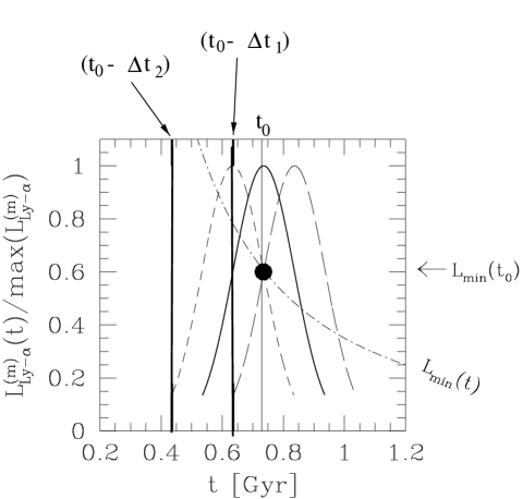
Figure 1: The constraint $t_{s}$ has to fulfill so that the Ly-$\alpha$ flux is detectable at $z_{0}$. The big black point marks the minimum flux detectable at $z_{0}=z(t_{0})$ with the detection limit $S_{lim}$. In order to be detectable in Ly-$\alpha$, the ignition epoch $t_{s}$ for the Ly-$\alpha$ emission has to be in the interval $[t_{0}-\Delta t_{2},t_{0}-\Delta t_{1}]$. This interval is marked by the thick vertical line. The short dashed, solid and long dashed curves show the possible Ly-$\alpha$ luminosity of PGs as a function of time with different ignition times $t_{s}$. The short dashed curve shows the time evolution of the Ly-$\alpha$ luminosity of a PG with an $t_{s}$ at the lower bound of the relevant time interval. At $t_{0}$ the Ly-$\alpha$ luminosity of such a PG is already very week e.g. because of ongoing dust formation. The solid curve corresponds to a PG with an ignition time $t_{s}$ centered in the relevant time interval. It reaches its maximal Ly-$\alpha$ luminosity at the epoch $t_{0}$ corresponding to the observed redshift $z_{0}$. Therefore, such a PG should be detectable. On the other hand, the long dashed curve corresponds to a PG with a $t_{s}$ at the right end of the relevant time interval. The Ly-$\alpha$ luminosity of such a PG has just reached detectable values and will rise further.

The maximal number of PGs in the volume $\Delta V_{c}$ which we can expect to be bright enough in Ly-$\alpha$ is then given by the integral over the mass function of PGs with lower integration limit $M_{min}$ multiplied by $\Delta V_{c}$:

$$\int_{M_{min}}^{\infty}\Phi(M,z_{0})dM\leavevmode\nobreak\ \Delta V_{c}$$ (3)

where the mass function $\Phi(M,z_{0})dM$ gives the comoving density of objects with mass $M\in[M,M+dM]$ at the observed redshift $z_{0}$.

But not all of these galaxies are in the PG phase at the observed epoch $t_{0}$. Some of them already left the PG phase or others enter this phase at a later epoch, so that they are dormant at $t_{0}$. The situation is illustrated in Fig. 1. The Ly-$\alpha$ bright phase during which a PG will be detectable in Ly-$\alpha$ is constrained to a certain time interval $[t_{s}+\Delta t_{1}(M),t_{s}+\Delta t_{2}(M)]$ which is defined by

$$\begin{array}[]{l}L_{Ly\alpha}^{(M)}(t-t_{s})\,\,\geq\,\,L_{min}(t_{0})\\ \\ \mbox{for all}\,t\in\,[t_{s}+\Delta t_{1}(M),t_{s}+\Delta t_{2}(M)]\end{array}$$ (4)

The PG is observable in Ly-$\alpha$ at $z_{0}=z(t_{0})$ only if $t_{0}\in[t_{s}+\Delta t_{1}(M),t_{s}+\Delta t_{2}(M)]$. This translates to a constraint for $t_{s}$:

$$t_{s}\,\,\in\,\,[t_{0}-\Delta t_{2}(M),t_{0}-\Delta t_{1}(M)]$$ (5)

Only PGs with $M\geq M_{min}$ which fulfill (5) will be detectable in Ly-$\alpha$ at a redshift of $z_{0}$ (Fig. 1).

The next building block of our model is the ’history of galaxy formation’, that is the distribution of ignition times $t_{s}$ which we assume to be coupled to the formation time of the halo. Galaxies show a substantial age spread. This translates to different $t_{s}$ for different galaxies. Finally our model should end up with the number of spheroids we observe today, e.g. with the current mass function of spheroids $\Phi(M,0)$. To take into account the ’history of galaxy formation’, we introduce a distribution function $P_{M}(t)dt$, which gives the fraction of current spheroids with mass $M$ which formed and started their first star formation during the time interval $[t,t+dt]$. The index $M$ indicates that $P_{M}(t)$ will in general depend on the mass of the objects. We normalize $P_{M}(t)$ according to

$$\int_{0}^{t(z=0)}P_{M}(t)dt=1$$ (6)

$t(z=0)$ is the present age of the universe.
$\Phi(M,0)\,P_{M}(t)dt\,dM$ gives the comoving number density of spheroids with mass in the mass interval $[M,M+dM]$ collapsing and starting their first star formation during the time interval $[t,t+dt]$. The number of PGs per solid angle $\Delta\omega$ with a detectable $Ly-\alpha$ flux above $S_{lim}$ is then given by

$$\begin{array}[]{l}N_{Ly_{\alpha}>L_{min}}(z_{0})=\\ \\ \int_{M_{min}(z_{0})}^{\infty}\left\{\int_{t_{0}-\Delta t_{2}(M)}^{t_{0}-\Delta t_{1}(M)}\Phi(M,0)P_{M}(t)dt\right\}dM\leavevmode\nobreak\ \Delta V_{c}(z_{0})\end{array}$$ (7)

Some remarks on equation (7):

• In this form, expression (7) is quite general but note that the integration limits $t_{0}-\Delta t_{2}(M)$ and $t_{0}-\Delta t_{1}(M)$ are determined by the duration of the phase in which the PGs of a certain mass are bright enough in Ly-$\alpha$ to be detectable. They depend strongly on the shape of the function $f(t-t_{s})$.

• The mass function (for spheroids) at redshift $z(t)$ is given by

  $$\Phi(M,z(t))=\Phi(M,0)\int_{0}^{t(z)}P_{M}(t)\,dt.$$ (8)

  With the normalization (6) we ensure that the number of spheroids which form in our model is the number we observe today.

• Note that with the normalization (6) we assume implicitly that the spheroids which form at high redshift remain until today and therefore we neglect that some spheroids might merge after their formation. This means that our approach might underestimate the abundance of PGs at intermediate $z$. This could in principle be dealt with by adjusting the right hand side of (6) to values $>1$. Because the merger rate might depend on the mass of the objects, these values would clearly be mass dependent. However, in this paper we keep the normalization constraint (6) for simplicity and therefore neglect merging of spheroids after their formation.

4 Discussion of two special cases

In order to make expression (7) more transparent, we choose two special functions for $P_{M}(t)$ and $L^{(M)}_{Ly\alpha}(t-t_{s})$. First, we assume for $P_{M}(t)$ a delta-function $P_{M}(t)=\delta(t-t_{in})$. That is, all spheroids have the same formation and ignition epoch $t_{s}=t_{in}$ and shine in Ly-$\alpha$ simultaneously (independent of their mass). If we assume that a fraction $\epsilon$ of the stars of a spheroid are born in the first starburst with a constant SFR over a period $\Delta t$ (that is $SFR=\epsilon M_{b}/\Delta t$, where $M_{b}$ is the stellar mass $\approx$ baryonic mass of the spheroid today) and that the Ly-$\alpha$ luminosity is proportional to the SFR, we get for the Ly-$\alpha$ luminosity

$$L^{(M_{b})}_{Ly\alpha}(t-t_{s})=\left\{\begin{array}[]{cc}k_{Ly\alpha}{\epsilon M_{b}\over{\Delta t}}&\mbox{\leavevmode\nobreak\ if \leavevmode\nobreak\ $t\in[t_{s},t_{s}+\Delta t]$}\\ 0&\mbox{otherwise}\end{array}\right.$$ (9)

With this choice for $P_{M}(t)$ and $L^{(M_{b})}_{Ly\alpha}(t-t_{s})$ (7) gives

$$\begin{array}[]{l}N_{det}(z_{0})=\\ \\ \left\{\begin{array}[]{cc}\int_{M_{min}(z_{0})}^{\infty}\Phi(M,0)dM\leavevmode\nobreak\ \Delta V_{c}(z_{0})&\,\mbox{ $t_{0}\in[t_{in},t_{in}+\Delta t]$}\\ 0&\,\mbox{otherwise}\\ \end{array}\right.\end{array}$$ (10)

This is the formula Baron & White (Baron87 (1987)) used for their calculations.

They took $t_{in}={1\over 5}t_{coll}$ and $\Delta t={4\over 5}t_{coll}$, where $t_{coll}$ is the duration of the collapse associated with a uniform spherical perturbation of the same initial mean density as the protogalaxy . They varied $z_{coll}$ between 6 and 1.5 and took $q_{0}=0.5$ and $q_{0}=0.05$. This corresponds to a variation of $\Delta t$ between 0.6 and 6 Gyrs. For the luminosity function $\Phi(L)$ of present-day galaxies they took a Schechter function with the parameters $\alpha=-1.25$, $L^{*}=1.6\times 10^{10}h_{0}^{-2}$L_⊙ and $\Phi^{*}=1.2\times 10^{-2}h_{0}^{3}$ Mpc^-3. Assuming (as we do) that one only can observe the ancestors of present-day ellipticals and the bulges of present-day spirals during their violent formation process, they reduced $\Phi^{*}$ by a factor of 3 to $0.4\times 10^{-2}h_{0}^{3}$ Mpc^-3. They used a mass-to-light ratio of 6.6 to convert the present day luminosity function to a mass function $\Phi(M,z_{0})$. To convert star formation rates into a Ly-$\alpha$ flux, they used for the constant $k_{Ly\alpha}$ in (9) the value $k_{BW}\,:=\,0.25\times 10^{35}{\mbox{W}\over{\mbox{m}^{2}}}{1\over{\mbox{M}_{\odot}\mbox{yr}^{-1}}}$. Note that this value is by a factor 4 smaller than the value deduced from local galaxies with the assumption of a standard IMF and CASE B recombination (Kennicutt Kennicutt83 (1983)). In this respect, Baron and White were conservative. Fig. 2 shows the results we got from (10) for $z_{0}=4.8$ and $\Delta z=0.1$ with the parameters of Baron & White together with the early limits from the Palomar Fabry-Perot survey for Ly-$\alpha$ emitting PGs (Thompson et al. 1995a , 1995b ) and more recent limits from CADIS (Maier et al. Maier02 (2003)) and LALA (Rhoads et al. Rhoads03 (2003)). Even the least optimistic predictions by Baron & White are in obvious conflict with the results of the latest surveys.

Figure 2: Most optimistic (solid line) and pessimistic (dashed line) number density predictions for Ly-$\alpha$ emitting PGs for $z_{0}=4.8$ and $\Delta z=0.1$ according to the parameters of Baron & White (1987) together with the early upper limits of the Palomar Fabry-Perot survey of Thompson et al. (1995a ) (triangles) and more recent searches by Maier et al. (Maier02 (2003)) (small arrows) and Rhoads et al. (Rhoads03 (2003)) (open star with arrow).

Alternatively, let us assume that the galaxies do not form and start at the same time with their Ly-$\alpha$ bright PG phase. A simple way to approximate this is to assume that the formation and ignition times $t_{s}$ of the galaxies are distributed equally over a certain time interval. So the delta function for $P_{M}(t)$ has to be replaced by the function

$$P_{M}(t)=\left\{\begin{array}[]{cc}{1\over{t_{out}-t_{in}}}=:{1\over{\Delta t_{P}}}&\mbox{if $t\in[t_{in},t_{out}]$}\\ 0&\mbox{otherwise}\end{array}\right.$$ (11)

Furthermore, we assume that the genuine Ly-$\alpha$ bright PG phase only lasts for a limited period, e.g. $\Delta t_{Ly\alpha}=0.2$ Gyr as discussed above:

$$L_{Ly\alpha}^{(M_{b})}(t-t_{s})\,=\,\left\{\begin{array}[]{ll}k_{Ly\alpha}{\epsilon\,M_{b}\over\Delta t}&\mbox{for $t\in[t_{s},t_{s}+\Delta t_{Ly\alpha}]$}\\ 0&\mbox{otherwise}\end{array}\right.$$ (12)

With (11) and (12) we get

$$\begin{array}[]{l}N_{Ly\alpha>L_{min}}(z_{0})\,=\\ \\ {\delta t\over{\Delta t_{P}}}\leavevmode\nobreak\ \int_{M_{min}(z_{0})}^{\infty}\Phi(M,0)dM\leavevmode\nobreak\ \Delta V_{c}\\ \\ \end{array}$$ (13)

with

$$\delta t\leq\Delta t_{Ly-\alpha}$$ (14)

Thus, in comparison with (10) the numbers are at least reduced by the factor $\Delta t_{Ly-\alpha}/\Delta t_{P}$. In Table 1 we show this factor for different $z_{in}$, $z_{out}$ ($z_{in}$ and $z_{out}$ are the redshifts, corresponding to $t_{in}$ and $t_{out}$ in (11)) and a $\Delta t_{Ly\alpha}$ of $2\times 10^{8}$ yr for different values of the matter density $\Omega_{M}$ and the vacuum energy density $\Omega_{V}$. Obviously the factors by which the numbers are reduced can be quite large. This simple example demonstrates that the predictions e.g. from Baron & White (Baron87 (1987)) are likely to be much too optimistic and could well over-predict the abundance of Ly-$\alpha$ bright galaxies by a factor of 10 or so.

Table 1: Factors $\Delta t_{Ly\alpha}/{\Delta t_{P}}$ for different $z_{in}$ and $z_{out}$ and $\Delta t_{Ly\alpha}=2\times 10^{8}yr$ (for $H_{0}=70\,\mbox{km/s Mpc${}^{-1}$}$).

$z_{in}$	$z_{out}$	$\Omega_{M}$	$\Omega_{V}$	$\Delta t_{Ly\alpha}\over\Delta t_{P}$
20	5	1.0	0.0	0.37
		0.3	0.0	0.23
		0.1	0.0	0.16
		0.3	0.7	0.20
		0.1	0.9	0.12
20	2	1.0	0.0	0.12
		0.3	0.0	0.08
		0.1	0.0	0.06
		0.3	0.7	0.07
		0.1	0.9	0.04

5 The detailed model

The above examples use oversimplified assumptions. A proper model instead should aim for more realistic functions $L^{(M)}_{Ly\alpha}(t)$, $P_{M}(t)$ and $\Phi(M,0)$. We deliberately follow a phenomenological approach: We try to parameterize the situation with reasonable functions and try to fix the parameters using both the present day galaxy population and some results from high redshift observations. Note the close similarity to the “semianalytic” models of galaxy evolution (see e.g. Somerville et al. Somverville01 (2001)).

5.1 The ’history’ of galaxy formation

In the previous section we approximated the function $P_{M}(t)$ by assuming that the ignition times $t_{s}$ of the galaxies are either fixed at a certain time or equally distributed over a time interval. Here we will estimate the function $P_{M}(t)$ from the paradigm that galaxies are assumed to arise from peaks in the density field $\delta(\@vec{x},t)=(\rho(\@vec{x},t)-\bar{\rho})/\bar{\rho}$. In the following we will omit the spatial coordinate $\@vec{x}$.

Consider the density field $\delta(M,t_{i})$ at an initial time $t_{i}$ smoothed with a box containing the mass $M$ and let $\sigma_{0}(M,t_{i})$ be the rms variation of this smoothed density field. We define the dimensionless fluctuation amplitude

$$\nu(M,t_{i}):={\delta(M,t_{i})\over{\sigma_{0}(M,t_{i})}}$$ (15)

In the linear regime the fluctuation amplitude grows proportionally to the linear growth factor $D(t)$. The density field at an epoch $t>t_{i}$, therefore, is given by

$$\delta(M,t)=\delta(M,t_{i})D(t)/D(t_{i})$$ (16)

The density contrast grows according to this simple relation until non-linear effects become important and the region ceases to expand, turns around and collapses to form a virialized halo. According to the linear relation (16) the density contrast would have reached a critical value $\delta_{c}$ at the time the halos form. $\delta_{c}$ can be estimated from the evolution of an isolated spherical over-dense region (see e.g. Padmanabhan (Padmanabhan93 (1993))). The value is of order one and depends weakly on $\Omega_{M}$. The exact value will not be important for our considerations. According to this rule, peaks in the initial density field (at epoch $t_{i}$ ) with a peak hight of $\nu(M,t_{i})=\delta_{c}D(t_{i})/(\sigma_{0}(M,t_{i})D(t_{0}))$ will collapse at the epoch $t_{0}$. We define the function

$$\nu_{i}(M,t):={\delta_{c}D(t_{i})\over{\sigma_{0}(M,t_{i})D(t)}}$$ (17)

We are interested in the number density $dN_{\mbox{form}}(t)$ of peaks which collapse in a certain time interval $[t_{0},t_{0}+dt]$. It depends on the distribution of the peak hights, $p(\nu)$. $p(\nu)d\nu$ gives the probability that a peak has a $\nu$-value in the interval $[\nu,\nu+d\nu]$. $p(\nu)$ translates into a distribution of collapse times. $dN_{\mbox{form}}(t)$ is given by

$$dN_{\mbox{form}}\sim p(\nu_{i}(M,t))\,\left|{d\nu_{i}\over{dt}}\right|\,dt$$ (18)

from which we obtain of the distribution in collapse times

$$P_{M}(t)=p(\nu_{i}(M,t))\left|{d\nu_{i}\over{dt}}\right|$$ (19)

The distribution of collapse redshifts is then given by

$$P_{M}(z)=p(\nu_{i}(M,t))\left|{d\nu_{i}\over{dt}}\right|\left|{dt\over{dz}}\right|$$ (20)

If we assume that we can approximate the fluctuation spectrum by a power-law with index $n$, we can write the function $\nu_{i}(M,t)$

$$\nu_{i}(M,t)=\left(M\over M_{*}\right)^{n+3\over 6}{D(t_{*})\over D(t)}$$ (21)

$M_{*}$ is the characteristic mass scale, which collapses at the time $t_{*}$. We treat $t_{*}$ for mass $M_{*}$ as a free parameter of our model. In this way we incorporate uncertainties in $\delta_{c}$ and the absolute normalization of the fluctuation power spectrum.

If the density fluctuation field is Gaussian, we can calculate the peak distribution $p(\nu)$ with the formalism given by Bardeen et al. (Bardeen (1986), BBKS). $p(\nu)$ depends on the width of the power spectrum under consideration. This is described by the BBKS parameter $\gamma$ ($\gamma=1$ corresponds to power at a single wavelength only; lower values indicate a larger range of wavelength). In the special case of a power-law spectrum with a Gaussian filtering $\gamma$ is given by (BBKS)

$$\gamma^{2}={n+3\over{n+5}}$$ (22)

Assuming a cold dark matter (CDM) model with adiabatic initial density fluctuations with a power spectrum $\sim k$, the power spectrum evolves as the universe expands into a power spectrum with effective power-law indices ranging from -3 on small scales up to 1 on large scales (see BBKS). On galactic scales the index is n=-2, which is the value we assume in the following. With Gaussian filtering (22) gives $\gamma=0.58$.

Figure 3: The distribution function $p(\nu)$ for $\gamma=0.58$ corresponding to an effective power-law index of the power spectrum of $n=-2$. The solid curve shows the result of the exact calculation and the dashed one is calculated with the fitting formula given by BBKS.

Since, in general, $p(\nu)$ cannot be written in closed form, BBKS give a fitting formula which is accurate enough for our purpose. Fig. 3 shows $p(\nu)$ for $\gamma=0.58$ calculated exactly and with the fitting formula provided by BBKS.
We normalize $P_{M}(t)$ according to equation (6). Fig. 4 shows the distribution $P_{M}(t)$ of the collapse times for three different masses $0.1*M_{*},M_{*}$ and $5\times M_{*}$. Fig. 5 shows the corresponding $P_{M}(z)$ curves. $t_{*}$ was chosen in such a way that $P_{M_{*}}(t(z))$ has its maximum at $z_{\mbox{max}}=z(t_{\mbox{max}})=6$. The curves illustrate again the crucial point of ’bottom up’ hierarchical structure formation: $P_{M}(t(z))$ with $M<M_{*}$ peaks at higher redshifts than $P_{M_{*}}(t(z))$ and $P_{M}(t(z))$ with $M>M_{*}$ peaks at lower redshifts than $P_{M_{*}}(t(z))$. Furthermore, the scatter (width) of the collapse times is smaller for small mass objects which form at high z than for massive objects which form later. Note that the peak formalism is not a strong theoretical motivation for the shape of our function $P_{M}(t_{s})$. By taking $z_{max}$ as a free parameter of the model (see above) we are not strictly applying the peak formalism which would give a definite result for the mass function of halos at a certain redshift once the power spectrum is known. Here we only use the peak formalism to get an estimate for the form of $P_{M}(t_{s})$. Furthermore remember that $t_{s}$ is not the formation time of the halo but the time when the first star formation starts whereas in the mass function which would be predicted directly by the peak formalism the variable would be the time of collapse $t_{col}$ of the halos. By using $z_{max}$ as a free parameter we leave open how exactly the collapse time and the ignition of star formation in halos are correlated. Comparison of our model with observations may in the end determine wether our choice for $P_{M}(t_{s})$ according to the paradigm of hirarchical structure formation was a good choice or not. However, because of the simplicity of our model, we could easily modify the function $P_{M}(t_{s})$ to take into account new results such as that bigger galaxies may have earlier star formation epochs as suggested by Heavens et al. (Heavens04 (2004)). This may be the subject of a following paper.

Figure 4: Distribution of collapse times for the three different masses $0.1\times M_{*}$ (dotted-dashed line), $M_{*}$ (solid line) and $5\times M_{*}$ (dashed line).

Figure 5: The same curves as in Fig. 4, but with the time axis transformed into redshift.

5.2 Development of the Ly-$\alpha$ luminosity with time

The assumption of a constant star formation rate and Ly-$\alpha$ luminosity of a PG as in (12) is a crude simplification. Detailed numerical simulations of the formation of galaxies (e.g. Steinmetz (Steinmetz93 (1993))) show that the SFR of PGs start with very low values, increase rapidly and reach a peak after a few $10^{8}$ years. The metallicity of the early bulge increases rapidly in this phase and soon reaches values around 1/10 of the solar value. According to our definition this limits the genuine Ly-$\alpha$ bright PG phase to a short time period $\Delta t_{Ly\alpha}$ of the order $10^{8-9}$ years. After this time the metalicity reaches values which inevitably lead to significant dust formation combined with an absorption of the Ly-$\alpha$ flux. Although the escape of Ly-$\alpha$ photons from star forming galaxies is a rather complicated problem depending on several conditions like the composition of the interstellar medium (e.g. multiphases, see Neufeld (Neufeld91 (1991)), or gas flows in the interstellar medium, see Kunth et al.  (Kunth99 (1999)) , we come back to this points in section 7), we simplify and assume that after a certain time period the Ly-$\alpha$ emission is no longer proportional to the SFR and decreases mainly due to the increasing dust content. We approximate this behavior by a Gaussian for $f(t-t_{s})$ (see (2) ) with a width $\sigma_{Ly\alpha}$ which remains a free parameter of our model:

$$\begin{array}[]{l}L^{(M_{b})}_{Ly\alpha}(t-t_{s})=\\ \\ \left\{\begin{array}[]{cc}k_{Ly\alpha}\cdot\epsilon\cdot{M_{b}\over{t_{s}}}\exp\left\{-{(t-t_{s}-2\sigma_{Ly\alpha})^{2}\over{2\sigma_{Ly\alpha}^{2}}}\right\}&\mbox{ for $t\geq t_{s}$}\\ 0&\mbox{otherwise}\\ \end{array}\right.\end{array}$$ (23)

Later on, we will see that the observed number densities of Ly-$\alpha$ emitting PGs constrains $\sigma_{Ly\alpha}$. The typical length of the Ly-$\alpha$ bright phase could be described by the FWHM $\Delta t_{Ly\alpha}=2\sigma_{Ly\alpha}\sqrt{2\ln 2}$ of (23). As already expressed in (2), we assume that the star formation rate and therefore the Ly-$\alpha$ flux during this first phase of star formation is proportional to the baryonic mass $M_{b}$ content of the galaxy. We further assume that $M_{b}$ is proportional to the total mass $M$ of the object according to $M_{b}={\Omega_{b}\over\Omega_{M}}M$ ($\Omega_{b}$ is the density parameter of the baryonic mass in the universe). Furthermore, we assume that the star formation rate and accordingly the Ly-$\alpha$ luminosity scales proportionally to $1/t_{s}$. This is motivated by the spherical collapse model (see e.g. Padmanabhan, Padmanabhan93 (1993)). A perturbation which decouples from the cosmic expansion at the epoch $t_{\mbox{max}}$ will collapse (to a black hole) at the epoch $t_{s}=2\times t_{\mbox{max}}$. The duration of the collapse process is therefore $\delta t=0.5\times t_{s}$. Hence, objects which collapse earlier collapse faster and we assume that the star formation rate is higher as well. Since we do not attempt to incorporate the complicated processes leading to primeval star formation and a certain IMF into our model, we summarize this in the free parameter $\epsilon$, which describes the overall scaling of the star formation with respect to $M_{b}$. As in our simple model in section 4 (see equation (9)) , $\epsilon$ can be interpreted as the factor of proportionality which determines the fraction of the stars of the spheroid which are born in the first starburst, although this is not strictly true as the Gauss function (23) describes the combined effect of star formation and dust production on the Ly-$\alpha$ emission. If all stars are produced in a very short starburst, $\epsilon$ could be well above 1. In this paper we fixed $\epsilon$ to one. This means that the Ly-$\alpha$ emission of a galaxy at its maximum corresponds to a SFR of $SFR={M_{b}\over{t_{s}}}$.

5.3 Mass function

We assume that

• Ly-$\alpha$ emitting PGs are the precursors of todays spheroids

• the baryonic mass we see today in these spheroids is proportional to the baryonic or total mass of the corresponding PG at the time of their first star formation

• subsequent merging processes or gas accretion does not destroy the luminous part of the average galaxy, which forms todays spheroid. However, merging of the PG into a larger halo (e.g. a cluster) may strip gas and/or the original dark halo of the galaxy and gas accretion might lead to the formation of a disk. Additional star bursts might add further stars to the spheroidal system, but the added baryonic mass is assumed to be proportional to the baryonic/total mass initially present at the time of the first star burst.

In equation (23) we therefore need the todays (baryonic) mass function of spheroids $\Phi_{\mbox{spheroids}}(M_{b},0)$. We derive the local bulge mass function from the type dependent luminosity functions determined from the CFA redshift survey by Marzke et al.  (Marzke94 (1994)) together with values for the type-dependent ratio of the bulge to disk luminosity from Simien & De Vaucouleurs (Simien86 (1986)) and a constant (baryonic) mass to light ratio for spheroids set to $10M_{\odot}/L_{\odot}$.

Marzke et al. (Marzke94 (1994)) described the luminosity functions for all Hubble types $T$ by Schechter functions

$$\Phi_{T}(L)dL\,=\,\Phi^{*}_{T}\left({L\over L^{*}_{T}}\right)^{\alpha_{T}}\exp\left\{-{L\over L^{*}_{T}}\right\}\,d\left({L\over L^{*}_{T}}\right)$$ (24)

with the parameters listed in table 2.

Table 2: Schechter function parameter for the different Hubble types according to Marzke et.al. (1994)

Hubble Typ T	$\alpha$	$L^{*}$	$\Phi^{*}$
		$[10^{9}h_{0}^{-2}L_{\odot}]$	$[10^{-3}h_{0}^{3}Mpc^{-3}]$
E  $T\in[-7,-4]$	-0.85	7.66	1.5
S0  $T\in[-3,0]\quad$	-0.94	4.88	7.6
Sa-Sb $T\in[1,4]$	-0.58	4.79	8.7
Sc-Sd $T\in[5,7]$	-0.96	5.2	4.4
Sm-Im $T>7$	-1.87	5.1	0.6

We write the total luminosity $L_{tot}$ of a galaxy as the sum of the bulge luminosity $L_{B}$ and the disk luminosity $L_{S}$:

$$L_{tot}\,=\,L_{B}\,+\,L_{S}$$ (25)

Furthermore, we denote with $\gamma_{T}$ the ratio of the bulge luminosity to the disk luminosity:

$$\gamma_{T}\,:=\,{L_{B}\over L_{S}}$$ (26)

The bulge mass of a galaxy of Hubble type T is given by

$$M_{B}\,=\,\Upsilon_{B}{1\over{1+\gamma_{T}^{-1}}}L_{tot}\,=:\,\Upsilon^{eff}_{T}L_{tot}$$ (27)

$\Upsilon_{B}$ denotes the mass-to-light ratio of the bulge components of present day galaxies, which is relatively independent of the galaxy type. We took $\Upsilon_{B}=10$ M_⊙/L_⊙. Eq. (27) defines $\Upsilon^{eff}_{T}$, a type dependent ”effective mass-to-light ratio”. Table 3 lists the values $\Upsilon^{eff}_{T}$ for different Hubble types calculated with the type dependent $\gamma_{T}$ values of Simien and DeVaucouleurs (1986).

Table 3: Effective bulge mass-to-light ratio $\Upsilon^{eff}_{T}$ for the different Hubble types.

Hubble Typ T	$\Upsilon^{eff}_{T}$
	$[M_{\odot}/L_{\odot}]$
E  $T\in[-7,-4]$	10
S0  $T\in[-3,0]$	5.4
Sa-Sb $T\in[1,4]$	2.8
Sc-Sd $T\in[5,7]$	0.48

$$M_{B}^{*}(T)\,=\,\Upsilon^{eff}_{T}\,L^{*}_{T}$$ (28)

With (28) the luminosity functions (24) transform into the type dependent bulge massfunctions

$$\begin{array}[]{l}\Phi_{T}(M_{B})dM_{B}\,=\\ \\ \quad\quad\Phi^{*}_{T}\left({M_{B}\over M_{B}^{*}(T)}\right)^{\alpha_{T}}\exp\left\{-{M_{B}\over M_{B}^{*}(T)}\right\}\,d\left({M_{B}\over M_{B}^{*}(T)}\right)\end{array}$$ (29)

The total (baryonic) spheroid mass function of present day galaxies is given by the sum over the mass functions of the different Hubble types

$$\Phi_{tot}(M_{B})\,dM_{B}\,=\,\sum_{T}\,\Phi_{T}(M_{B})\,dM_{B}$$ (30)

We will use (30) as an approximation for the mass function $\Phi(M_{b},0)$ in equation (7).

5.4 Summary of the model

We constructed a phenomenological model to calculate the expected surface density of Ly-$\alpha$ emitting, high redshift young galaxies. According to (7) we have to take into account the evolution of the Ly-$\alpha$ luminosity as a function of time and mass of the galaxy and the galaxy formation history. We estimated these functions with the following assumptions:

• We assume that Ly-$\alpha$ emitting PGs are the precursors of the present day spheroids (=bulges & ellipticals) in the phase of their first star burst.

• The first star formation starts in a dust-free environment. The enrichment of the IGM with dust in the first hundred million years of star formation leads to a rapid attenuation of the Ly-$\alpha$ emission. The time evolution of the Ly-$\alpha$ emission is described by a Gaussian with FWHM $\Delta t_{Ly\alpha}$, which gives the typical duration of the Ly-$\alpha$ bright phase.

• The SFR and accordingly the Ly-$\alpha$ emission is assumed to be proportional to the baryonic mass $M_{b}$ of the PG. Furthermore, the SFR is assumed to scale with $1\over t_{s}$, where $t_{s}$ is the collapse time: Comparing objects with the same baryonic mass, the ones which form their stars at higher redshifts have higher star formation rates.

• We get a first guess for the functional form of the distribution of ’ignition times’ $P_{M}(t_{s})$ by the distribution of peak hights $p(\nu)$. However, this is a mere ad-hoc assumption with no strong theoretical motivation. We fix the parameters $M_{*}$ and $t_{*}$ so that $P_{M}(t_{s})$ peaks at a certain redshift $z_{\mbox{max}}$ for $M=M_{*}=4\times 10^{10}$M_⊙, which corresponds roughly to the (baryonic) bulge mass of our Milky Way. $z_{\mbox{max}}$ is a free parameter of our models.

• We normalized $P_{M}(t_{s})$ so that our model ends up at $z=0$ with the mass function of spheroids we see today. This assumes that the spheroids which formed in the early universe stay as entities until today and that their current baryonic mass is proportional to the baryonic mass at the time of their first star formation. This does not exclude later merging processes of the dark matter halos and e.g. accretion of gas, which may lead to the formation of a disk.

An overview of parameters of our model is given in Table 4. Note that we keep those parameters fixed which are determined by observations of the local universe or theoretical arguments. The free parameters of our model have to be determined by the observational statistics of Ly-$\alpha$ bright PGs. This will be attempted in paper II. Here we will only point to the most obvious constraints (see section 7.2) and use them to define a “basic model”. In Table 4 the parameter values of this “basic model” are summarized.

Table 4: Parameters of the model and their value range explored in this paper. The values of the “basic model “ are chosen in such a way that the model is in agreement with recent observations (see section 7.2 )

Parameter	Value range	Explanation	“Basic Model”
$\Omega_{M},\Omega_{\lambda}$	$\Omega_{M}=1.0$, $\Omega_{\Lambda}=0.0$	flat CDM (fCDM)
	$\Omega_{M}=0.3$, $\Omega_{\Lambda}=0.0$	open CDM (oCDM)
	$\Omega_{M}=0.3$, $\Omega_{\Lambda}=0.7$	$\Lambda$ CDM	$\Omega_{M}=0.3$, $\Omega_{\Lambda}=0.7$
h	0.7	Hubble paramter $H_{0}=h100$km /s Mpc-1	0.7
$\Delta t_{Ly\alpha}=2\sigma_{Ly\alpha}\sqrt{2\ln 2}$	0.1 - 2 Gyr	duration of the Ly-$\alpha$ bright phase	0.35 Gyr
$\epsilon$	$\epsilon\equiv 1$	star formation effiency	1
$n$	-2.0	power law index of the power spectrum	-2.0
$z_{max}$	3-25	redshift, at which the distribution of	3.4
		’ignition times ’ $P_{M}(t_{s})$ peaks for
		$M=M_{*}=4\times 10^{10}\mbox{M}_{\odot}$
$\alpha$,$L^{*}$, $\Phi^{*}$, $\Upsilon^{eff}$	see Table 2 and Table 3	parameters describing the luminosity function and	see Table 2 and
		the mass to light ratio for todays spheroids	Table 3

Figure 6: Expected number density per deg² and $\Delta z=0.1$ of Ly-$\alpha$ emitting PGs with a minimum detectable Ly-${\alpha}$ flux of $S_{lim}=3\times 10^{-20}$Wm^-2. $\Delta t_{Ly\alpha}$ was fixed to 0.35 Gyr according to our “basic model”. The different panels show the results for different observing redshifts $z_{0}$. The three different curves in each panel correspond to different cosmologies: The solid line corresponds to $\Omega_{M}=0.3$, $\Omega_{\Lambda}=0.0$, the dashed line corresponds to $\Omega_{M}=1.0$, $\Omega_{\Lambda}=0.0$ and the dashed dotted line corresponds to $\Omega_{M}=0.3$, $\Omega_{\lambda}=0.7$.

6 Predicted abundance of Ly-${\alpha}$ galaxies

Fig. 6 shows the expected number density of Ly-$\alpha$ emitting PGs as a function of $z_{\mbox{max}}$. The different panels show the results for different observing redshifts $z_{0}$. Note that the curves for the different redshifts look very similar. They rise steeply at small $z_{max}<z_{0}$ to a maximum and then fall off slowly at high redshifts $z_{max}>z_{0}$. This behavior can be understood by Fig. 7 which shows $P_{M}(z)$ for elliptical galaxies with $M=M_{*}$ and various $z_{max}=3,\leavevmode\nobreak\ 6,\leavevmode\nobreak\ 9$ and 12. The two vertical solid lines mark the interval (5) for $z_{0}=3.5$. The number of observable Ly-$\alpha$ emitting PGs is proportional to the shaded area under the $P_{M}(z)$ curve in this interval. The observed number density is governed by two effects: For low $z_{max}$ the maximum of the $P_{M}(z)$ curve lies on the left hand side of the interval (5), that is at redshifts below $z_{0}$ (see the solid curve in Fig. 7). With decreasing $z_{max}$ the width of the $P_{M}(t)$ curve increases rapidly. This corresponds to an increasing spread of the ignition times, that is an increasing $\Delta t_{P}$ in (11) (see also the discussion there). Taking into account the normalization constraint (6), the overall amplitude of $P_{M}(z)$ decreases rapidly with decreasing $z_{max}$. This explains the steep decrease of the curves in Fig. 6 for decreasing $z_{max}<z_{0}$.

If $z_{max}$ lies at higher redshift than the interval (5) we face the following situation: With increasing $z_{max}$ the overall amplitude of $P_{M}(z)$ increases rapidly (see the dashed, dotted and dashed dotted lines in Fig. 7).The reason for this is that the width of the curves $P_{M}(t)$ decreases with increasing $z_{max}$. However, because the total number of galaxies which form is conserved (see again (6)) the total area under the $P_{M}(t)$ curve does not change much. Thus, the peak amplitudes of $P_{M}(t)$ and $P_{M}(z)$ increase. This almost completely compensates for the effect that for $z_{max}>z_{0}$ the observed redshift interval (see Fig. 7) samples lower and lower relative levels of the $P_{M}(z)$ curve. If one does not consider one specific mass only but the full range of masses $M>M_{lim}$, the situation becomes somewhat more involved but the basic explanation for the behavior of the $N(z_{max})$ curves remains valid.

The lines in the different panels of Fig. 6 reach roughly the same maximum value $N_{max}$, almost independently of the observation redshift $z_{0}$. For instance, for $\Omega_{m},\Omega_{\Lambda}=0.3,0.7$, we find $1200<N_{max}<1600/\squareforqed\degr/(\Delta z=0.1)$ out to redshift $z_{0}=9.3$. This can be understood in the following way: (1) Because we assumed that the star formation rate and accordingly the Ly-$\alpha$ flux scales proportional to $1/t_{s}$ (see eq. (23)), galaxies of a given mass are intrinsically brighter in Ly-$\alpha$ if they form at higher redshift. (2) As discussed above, the function $P_{M}(t)$ is narrower if it peaks at higher redshifts (see Fig. 4 and Fig. 5) and thus exhibits a higher peak amplitude.

(3) In addition one should note that the comoving volume $\Delta V(z)$ is almost independent of $z$ between $z\approx 3$ and $z\approx 6$.

(1) and (2) lead to an increase of PGs above a fixed mass limit with increasing $z_{0}$. On the other hand, increasing $z_{0}$ means increasing the luminosity distance $d_{L}$ of the observed objects, and thus requires higher masses for PGs which are still observable above the detection limit $S_{lim}$. Since both $t(z)$ and $D_{L}(z)$ directly depend on the geometry of the universe, the fact that $N_{max}$ is almost independent of $z_{0}$ is not a coincidence but rather a genuine property of our model.

After to $z_{max}$, the least known free parameter of our model is the duration of the Ly-$\alpha$ bright phase, $\Delta t_{Ly\alpha}$. Actually, it depends on the detailed astrophysical conditions during the formation of the first generation of massive stars in PGs. Most notable are the initial mass function (IMF) which determines the rate of heavy element production, the feedback processes which enrich the interstellar gas, the cooling of the hot gas phase, the topology of the star forming regions and many more. Therefore it is essential to understand how $\Delta t_{Ly\alpha}=2\sqrt{2\ln 2}\cdot\sigma_{Ly\alpha}$ influences the predicted number of Ly-$\alpha$ galaxies in our model.

The panels in Fig. 8 show the expected number density of Ly-$\alpha$ emitting PGs as a function of $\sigma_{Ly\alpha}$ for a survey flux limit $S_{\rm lim}=3\times 10^{-20}\,\mbox{W/m${}^{2}$}$. From equation (23) we get for the length $\Delta t$ of the time interval (5)

$$\Delta t=\Delta t_{2}\,-\,\Delta t_{1}=2\,\sigma_{Ly\alpha}\sqrt{2\ln\left(M\over{M_{min}}\right)}$$ (31)

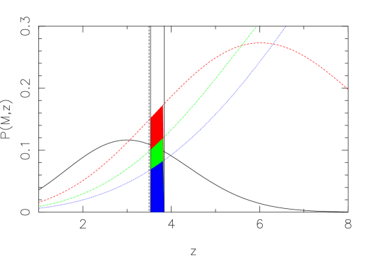
Figure 7: $P_{M}(t)$ for elliptical galaxies with $M=M_{*}$ and different $z_{max}=3,6,9$ and 12.The two vertical lines mark the interval (5) for $z_{0}=3.5$. The dashed vertical line very close to the left border of the interval (5) marks the observing redshfit $z_{0}=3.5$.

First, we consider the case $\sigma_{Ly\alpha}<<t(z_{0})$, $z_{max}\geq z_{0}$. In this case the time interval (5) ends shortly before $t(z_{0})$ and the maximum of the $P_{M}(t)$ curve is located at higher redshifts than the redshift corresponding to ($t_{0}-\Delta t_{2}$) (see Fig. 7). An increase of $\sigma_{Ly\alpha}$ has two effects which both increase the expected number density of Ly-$\alpha$ emitting PGs:

• The interval (5) over which $P_{M}(t)$ is integrated increases proportional to $\sigma_{Ly\alpha}$

• The interval (5) moves to the right, that is nearer to the maximum of $P_{M}(t)$.

If $z_{max}<z_{0}$ and $\sigma_{Ly\alpha}<<t(z_{0})$ the increase of the interval (5) proportional to $\sigma_{Ly\alpha}$ gives an increase of the expected number density, too. Accordingly, all curves in Fig. 8 have a positive slope at small $\sigma_{Ly\alpha}$. On the other hand, if $\sigma_{Ly\alpha}$ is large, the interval (5) moves to earlier times before $P_{M}(t)$ reaches its maximum and where $P_{M}(t)$ is a steep function of $t$. This leads to a decrease of the expected number density of Ly-$\alpha$ emitting PGs when further increasing $\sigma_{Ly\alpha}$.

Figure 8: Expected number density per deg² and $\Delta z=0.1$ of Ly-$\alpha$ emitting PGs as a function of $\sigma_{Ly\alpha}$ (see 23) for fixed $S_{lim}=3\times 10^{-20}\mbox{W/m${}^{2}$}$. The cosmology is fixed to $\Omega_{M}=0.3$, $\Omega_{\Lambda}=0.7$. The solid curves correspond to $z_{max}=3.4$, the dashed curves to $z_{max}=6$ and the dotted dashed curves to $z_{max}=10$.The arrow marks the value $\sigma_{Ly-\alpha}=0.15$ of our “basic model”.

Figure 9: Expected number density per deg² and $\Delta z=0.1$ of Ly-$\alpha$ emitting PGs as a function of the minimum detectable Ly_α flux of $S_{lim}$ according to our “basic model” parameters $\Delta t_{Ly-\alpha}=0.35$ Gyr and $\Omega_{M}=0.3$, $\Omega_{V}=0.7$. The solid curves correspond to $z_{max}=3.4$, the dashed curves to $z_{max}=6$ and the dashed dotted curves to $z_{max}=10$.

Finally, we show the expected abundance of Ly-${\alpha}$ galaxies as function of the survey limit $S_{lim}$ and observed redshift $z_{0}$ (see Fig. 9). For the purpose of this plot we fixed the duration of the Ly-${\alpha}$ bright phase to the value of our basic model: $\Delta t_{Ly\alpha}=0.35$ Gyrs (see section 7.2). To illustrate the dependence on $z_{max}$ we display the cumulative number density of Ly-$\alpha$ emitting PGs for three different values of $z_{max}=3.4,6.0$ and $10.0$. It is obvious from Fig. 9 that for $z_{max}\la 10$ a set of optical surveys for Lyman-$\alpha$ ($z_{0}=3.5$ corresponds to $\lambda({\rm Ly}\alpha)=547$ nm, $z_{0}=6.6$ to 924 nm) could be sufficient to determine $z_{max}$. However, when $z_{max}$ is located beyond $z_{max}=10$, only the inclusion of a deep near infrared emission line survey (e.g. in the J band aiming for Ly-$\alpha$ at $z_{0}\simeq 9.3$) would be conclusive. Such a survey seems not feasible from the ground and would have to wait for the Next Generation Space Telescope.

7 Discussion

After we outlined the generic properties and predictions of our model, we discuss several aspects which relate to current and future surveys for Ly-$\alpha$ emitting primeval galaxies.

7.1 Optimum survey strategy

First, we consider what conclusions about an optimum survey strategy for Ly-$\alpha$ galaxies can be drawn from the predicted number densities (Fig. 9): At bright detection limits (e.g. $\log(S_{\rm lim})\ga-19.5$ for $z_{0}<6$ ) the curves are steep due to the exponential fall-off of the underlying luminosity function (i.e. underlying mass function (30)) towards high luminosities. Here it will be more useful to improve the detection limit of a survey than to enlarge its area. The opposite is true at very faint detection limits (e.g. $\log(S_{\rm lim})\la-20.5$ for $z_{0}<6$). A survey which reaches such a depth will benefit more from an increase in area than from pushing the limits deeper.

Formally, one might quantify the merit of a Ly-$\alpha$ survey by the total number $N_{\rm PG}$ of Ly-$\alpha$ emitting PGs which could be found by spending a given observing time $t_{obs}$ at a given telescope.

Using the observing time $t_{obs}$ to increase the observed area $\Delta\omega$ on the sky gives

$$\begin{array}[]{rl}N_{\rm PG}\propto\Delta\omega&\propto t_{obs}\\ &\\ \Rightarrow\log(N_{\rm PG})&=\log(t_{obs})+const.\\ &\\ \Rightarrow{\partial\log(N_{\rm PG})\over\partial\log(t_{obs})}&=1\end{array}$$ (32)

On the other hand, using observing time to improve the detection limit $S_{\rm lim}$:

$$\begin{array}[]{rl}S_{\rm lim}&\propto{1\over\sqrt{t_{obs}}}\\ &\\ \Rightarrow\log(S_{\rm lim})&=-{1\over 2}\log(t_{obs})\,+\,const.\end{array}$$ (33)

If we take into account that $\log(N_{\rm PG})$ is a function of $S_{\rm lim}$

$$\log(N_{\rm PG})\,=\,f(\log(S_{\rm lim}))\,=\,f\left(-{1\over 2}\log(t_{obs})+const\right)$$ (34)

we find:

$$\begin{array}[]{rl}{\partial\log(N_{\rm PG})\over\partial\log(t_{obs})}&=\,f^{\prime}(\log(S_{\rm lim}))\,{\partial\log(S_{\rm lim})\over{\partial\log(t_{obs})}}\\ &\\ &=-{1\over 2}f^{\prime}(\log(S_{\rm lim}))\end{array}$$ (35)

Notice that $f^{\prime}<0$ everywhere (cf. Fig. 9). Comparison of (32) and (35) shows how the optimum survey strategy should be chosen: If $f^{\prime}(\log(S_{\rm lim}))<-2$ one should use additional observing time to increase the integration time in order to reach fainter flux limits. If $f^{\prime}(\log(S_{\rm lim}))\geq-2$ additional observing time should be used to increase the survey area $\Delta\omega$ on the sky in order to increase the number density of detectable PGs.

Figure 10: Comparison of our “basic model” with observational data. Big open star: LALA survey of Rhoads et al. (Rhoads03 (2003)); filled square: Hu et al. (Hu99 (1999)); small stars and arrows: CADIS Maier et al. (Maier02 (2003)); open boxes: Hu et al. (Hu98 (1998));open circles: Kudritzki et al. (Kudritzki00 (2000)); filled star with arrow: LALA survey of Rhoads et al. Rhoads03 (2003) for $z_{0}=4.8$; solid line: $z_{0}=3.5$; dashed line: $z_{0}=5.7$; dotted dashed line: $z_{0}=4.8$;

Figure 11: Expected number density per deg² and $\Delta z=0.1$ of $Ly-\alpha$ emitting PGs as a function of the observation redshift $z_{0}$ for $\Delta t_{Ly\alpha}=2\sigma_{Ly-\alpha}\sqrt{2\ln 2}=0.35$ Gyr (according to our “basic model”) at a detection limit of $lg(S_{lim}[\mbox{W/m${}^{2}$}])=-19.5$. The three curves correspond to $z_{max}=3.4$ (solid curve) ,4.5 (dashed curve), 5.5 (dashed dotted curve). The cosmology is fixed to $\Omega_{M}=0.3$, $\Omega_{V}=0.7$ (according to our “basic model”). The symbols mark observational data: open box: Hu et al. (Hu98 (1998)) for $log(S_{lim}[\mbox{W/m${}^{2}$}])=-19.5$; open circle: Kudritzki et al. (Kudritzki00 (2000)) for $log(S_{lim}[\mbox{W/m${}^{2}$}])=-19.5$; small star: CADIS Maier et al. (Maier02 (2003)) for $log(S_{lim}[\mbox{W/m${}^{2}$}])=-19.54$.

Figure 12: Expected number density per deg² and $\Delta z=0.1$ of $Ly-\alpha$ emitting PGs as a function of the observation redshift $z_{0}$ for $\Delta t_{Ly\alpha}=2\sigma_{Ly-\alpha}\sqrt{2\ln 2}=0.35$ Gyr and the detection limits of $log(S_{lim}[\mbox{W/m${}^{2}$}])=$ -21.0 (solid line), -20.0 (dashed line), -19.0 (dashed dotted line). $z_{max}$ is fixed to 3.4 and the cosmology is fixed to $\Omega_{M}=0.3$, $\Omega_{V}=0.7$ (according to our “basic model”). The symbols mark observational data: open box: Hu et al. (Hu98 (1998)) for $log(S_{lim}[\mbox{W/m${}^{2}$}])=-19.1,-19,9$; open circle: Kudritzki et al. (Kudritzki00 (2000)) for $log(S_{lim}[\mbox{W/m${}^{2}$}])=-19.0,-19.8$; small stars: CADIS Maier et al. (Maier02 (2003)) for $log(S_{lim}[\mbox{W/m${}^{2}$}])=-19.54,-19.32,-19.19$.

7.2 Comparison with observed abundance

We have chosen the parameters of our “basic model” in such a way that our model fits the observed surface density of Ly-$\alpha$ emitting PGs at redshifts $z_{0}=3.5$ and $z_{0}=5.7$. Fig. 10 shows the result. If we keep $\epsilon$ fixed to $1$ the main free paramters of the model are $z_{max}$ and $\Delta t_{Ly-\alpha}$. These parameters seem to be strongly constrained by the observational data at different redshifts. To produce Fig. 10 we varied the two parameters $z_{max}$ and $\Delta t_{Ly-\alpha}$ by hand in order to fit the data. It is non trivial to find a combination of values consistent with all available data. However, as explained below, part of the difficulty may arise from a second Ly-$\alpha$ bright phase of PGs.
Fig.11 shows the surface density of Ly-$\alpha$ emitters as a function of redshifts $z_{0}$ for different $z_{max}$ and a fixed detection limit. Fig. 12 shows the same diagram for different detection limits $\log(S_{lim}[\mbox{W/m${}^{2}$}])=$-21, -20, -19 but fixed $z_{max}=3.4$. At faint detection limits $\log(S_{lim}[\mbox{W/m${}^{2}$}])<-20.0$ the number density peaks at redshifts $z_{0}\geq 3$ and falls off slowly with increasing redshift. For $z_{max}=$4.5 and 5.5 the surface density of Ly-$\alpha$ emitters at a detection limit of $\log(S_{lim}[\mbox{W/m${}^{2}$}])<-20.0$ is expected to be more or less constant in the redshift range $z_{0}=3...5$ with values $\geq 10^{3}$ 1/deg² / $\Delta z=0.1$, reaching its maximum at $z_{0}\approx 4$. For $z_{max}=3.4$ the surface density falls faster with increasing redshift $z_{0}>3$, especially at lower detection limits. However, at faint enough detection limits, $\log(S_{lim}[\mbox{W/m${}^{2}$}])\approx$-21 (see Fig. 12), the number density only changes moderately in the redshift range between 3 and 5. At faint detection limits $\log(S_{lim}[\mbox{W/m${}^{2}$}])<-20.0$ the expected number density of Ly-$\alpha$ emitting PGs is expected to be significantly higher ($\geq\mbox{several}\,\,100$ / deg² / $\Delta z=0.1$) out to very high redshifts of $z_{0}\approx 8$. This may open interesting prospects for the examination of the epoch of reionisation (see Haiman, Haiman02 (2002) and Cen, Cen03 (2003)). On the other hand according to Fig. 12 the surface density of Ly-$\alpha$ emitting PGs is predicted to be a steep function of observing redshfit $z_{0}$ and detection limit at high detection limits $\log(S_{lim}\mbox{W/m${}^{2}$}])\geq-19$ which explains the failure of early surveys (see Pritchet et al. Pritchet94 (1994)).

As we determined the model parameters only with the data at $z_{0}=3.5$ and $z_{0}=5.7$ we get an independent prediction for the surface density of Ly-$\alpha$ emitting PGs at e.g. $z=4.8$ (see Fig. 10). According to this prediction, the surface density at $z=4.8$ e.g. at $\log(S_{lim}[\mbox{W/m${}^{2}$}])=-19.5$ should be roughly a factor of 4 higher than at $z=5.7$. But very recent data by the LALA survey (Rhoads et al. Rhoads03 (2003)), CADIS survey (Maier et al. Maier02 (2003)) and the Subaru Deep Field survey (Shimasaku et al. Shimasaku03 (2003)) indicate that the surface density of Ly-$\alpha$ emitting PGs does not differ much between $z=4.8$ and $z=5.7$ at $\log(S_{lim}[\mbox{W/m${}^{2}$}])=-19.5$. As we will discuss in detail in paper II, this can be understood in the framework of our models if $z_{max}$ is close to 5 or 6 instead of 3.4 (cf. Fig. 11 for the case $z_{max}=5.5$). However, the low absolute numbers observed at $z_{0}=5.7$ and $z_{0}=4.8$ can then only be explained by reducing either $\epsilon$ or $\sigma_{Ly\alpha}$ considerably. As this will also reduce the absolute numbers at $z_{0}=3.5$ a conflict with the observations is unavoidable. This might be a hint that a large fraction of the Ly-$\alpha$ emitters at $z_{0}<4$ do not belong to the class of “primeval” Ly-$\alpha$ galaxies considered here, but are galaxies in a later state of evolution (see section 7.4)

7.3 Comparison with other models

Besides the calculations of Haiman and Spaans (Haiman99 (1999)) our calculations are the only ones that try to model the number density of Ly-$\alpha$ emitters at high redshifts taking into account the formation of dust during the early phases of star formation and the history of galaxy formation. Haiman and Spaans deduced the mass function and formation history of haloes directly from the power spectrum with the Press-Schechter formalism, whereas we extrapolated the local luminostiy function of galaxies and their stellar content back into the past and only used the power spectrum and peak formalism to deduce a realistic distribution of formation times. Furthermore, while we use a phenomenological approach to describe the modulation of the Ly-$\alpha$ emission by dust formation in the early phase of star formation, Haiman and Spaans used detailed Monte Carlo simulations of individual galaxies with a range of masses for the ionizing stars, dust content and inhomogeneity together with the solutions of the radiative transfer problem for the Ly-$\alpha$ line in an inhomogeneous multi-phase medium (Neufeld, Neufeld91 (1991)). It is interesting that our model and the model of Haiman and Spaans both agree in predicting high surface densities of Ly-$\alpha$ emitters out to redshifts $\approx 8$. Furthermore, both models also predict that the surface density of Ly-$\alpha$ emitters as a function of redshift at faint detection limits (see Fig. 12) should be rather flat in the redshift interval between 4 and 6.

7.4 Lyman-break galaxies and second generation Ly-$\alpha$ emission.

In our models we assumed that strong Ly-$\alpha$ emitting PGs are young spheroids during their very first phase of star formation in which dust does not play a crucial role. Subsequently the interstellar medium will be enriched with metals very soon after the onset of star formation. Due to the ongoing dust formation, Ly-$\alpha$ photons will be more and more absorbed. The Ly-$\alpha$ flux of the PGs will decrease although the SFR may still increase and reach its maximum at a later time. A Ly-$\alpha$ dark phase follows, during which all Ly-$\alpha$ photons are destroyed due to resonant scattering in the dusty interstellar medium and during which the SFR reaches its maximum.

At later times after the SFR reaches its maximum, model calculations (see e.g. Friaça and Terlevich (Friaca99 (1999))) predict a phase in which strong outflowing winds build up. Once these winds have developed, a second Ly-$\alpha$ bright phase might develop. Complicated outflows of gas with high velocities $v$ are indeed a common feature of LBGs (see Pettini et al. Pettini98 (1998)) and have also been found in nearby HII galaxies (Kunth et al. Kunth98 (1998)). Large scale outflows not only explain that whenever LBGs show Ly-$\alpha$ in emission, this is shifted by up to $\approx 1000$km/s relative to the metal absorption lines but in addition explain their P-Cygni line profiles.
The Ly-$\alpha$ line of objects in this second Ly-$\alpha$ bright phase should be shifted by the velocity of the outflowing wind relative to the metal absorption lines and should show a P-cygni profile. In principle high resolution high S/N spectra of the objects may allow us to disentangle Ly-$\alpha$ emitting objects which are in their first or second Ly-$\alpha$ bright phase. In our predictions for the number density of Ly-$\alpha$ emitters we took into account only the first Ly-$\alpha$ bright phase and neglected the possible second phase. At very faint detection limits and redshift $z_{0}<4$, Ly-$\alpha$ emitters from the second phase might contribute. However, because we fixed our parameters to the observed surface density of Ly-$\alpha$ emitters by Hu et al.(Hu98 (1998)) and the new CADIS (Maier et al. Maier02 (2003)) results, which do not distinguish between two Ly-$\alpha$ emitting phases of PGs, our value for $\Delta t_{Ly\alpha}$ might be representative of a (weighted) sum of the durations of both phases. In this, the duration of the second phase might have a lower weight, because this phase might be much fainter in Ly-$\alpha$ than the first one. Furthermore, one would expect that the relative “contamination” by Ly-$\alpha$ emitters in this second Ly-$\alpha$ bright phase increases with time. This might explain why Ly-$\alpha$ emitters at $z_{0}=3.5$ seem overabundant in comparison to a model which fits their density at redshifts $z_{0}>4.5$.

8 Conclusions

We presented a simple phenomenological quantitative model for the expected surface number density of high redshift Ly-$\alpha$ emitting galaxies. We assumed that elliptical galaxies and bulges of spiral galaxies (which we call spheroids) formed early in the universe while disks were built up at a later stage. Thus, we identified the high redshift Ly-$\alpha$ emitting PGs with these spheroids during their first burst of star formation. One of the main assumptions of our model is that the Ly-$\alpha$ bright phase of this first starburst is confined to the first several hundred million years after the onset of star formation (duration: $\Delta t_{Ly\alpha}$). We assumed an ad-hoc-function for the distribution of ’ignition times’ with some motivation from the distribution of peak hights in the peak-formalism. In order to derive absolute number densities, we follow the method backwards in time as pioneered by Baron & White (1987): The number of PGs that form in our model are normalized to the present (baryonic) mass function of spheroids. Using the surface density of Ly-$\alpha$ emitters detected by recent surveys at redshifts 3.5 and 5.7, we find that the Ly-$\alpha$ bright phase of primeval galaxies is very likely confined to a rather short period of $\leq 0.5$ Gyr after the onset of star formation. Our model predicts that the surface density of Ly-$\alpha$ emitters with Ly-$\alpha$ fluxes $S_{\mbox{lim}}\leq 10^{-20}$W/m² should be high ($\geq\mbox{several}\,\,100/\squareforqed\degr/(\Delta z=0.1)$) out to very high redshifts of $z_{0}\approx 8$. The substantial number of spectroscopically confirmed high redshift Ly-$\alpha$ emitting objects at redshifts $z_{0}\geq 5$ (see e.g. Santos et al. Santos04 (2004) or Malhotra and Rhoads Malhotra04 (2004) and references therein) show that systematic searches for these objects are indeed successful. Now the main task for observers will be to quantify the selection effects and to separate the second generation Ly-$\alpha$ emitters. Together with our simple phenomenological model the observation of the Ly-$\alpha$ luminosity function at high redshifts (e.g. $z=5.7,6.6,9.3,12.6$ as discussed above) may give interesting hints concerning the peak of galaxy formation activity (from $z_{max}$) and the duration of Ly-$\alpha$ bright phases of PGs (from $\Delta t_{Ly-\alpha}$). As soon as this is accomplished our model will be able to pin down the formation of galaxies in term of the three parameters $\epsilon,\Delta t_{Ly-\alpha}$ and $z_{max}$. It will be straightforward to test any physical model of galaxy formation with respect to this intuitive parameterisation of the observed abundance of PGs.

- (1) Bardeen, J.M. et al., 1986, ApJ, 304, 15
- (2) Baron, E. and White, S., 1987, ApJ, 322, 585
- (3) Cen, R., 2003, ApJ, 597, L13
- (4) Charlot, S. & Fall, S., 1993, ApJ, 415, 580
- (5) Dey, A. et al., 1998, ApJ, 498, L93
- (6) Friaça, A.C.S. & Terlevich, R.J., 1999, MNRAS, 305, 90
- (7) Haiman, Z. and Spaans, M., 1999, ApJ, 518, 138
- (8) Haiman, Z., 2002, ApJ, 576, L1
- (9) Heavens, Panter, Jimenez, Dunlop, astro-ph/0403293
- (10) Herbst, T.M. 1994, PASP 106, 1298
- (11) Hippelein, H. et al. 2003, A& A, 402, 65
- (12) Hu, E.M., Cowie, L.L., McMahon, R.G., 1998, ApJ 502, L99
- (13) Hu, E.M., McMahon, R.g., Cowie, L.L. 1999, ApJ, 522, L9
- (14) Hu, E.M. et al. 2002, ApJ, 568, L75
- (15) Hu, E.M. et al. 2003, astro-ph/0311528
- (16) Kennicutt, R.C.,1983, ApJ, 272, 54
- (17) Kudritzki, R.-P., Mendez, R.H., Feldmeier, J.J. et al. 2000, ApJ, 536, 19
- (18) Kunth, D. et al., 1998, A&A, 334, 11
- (19) Kunth, D., et al., 1999, to appear in Thuan T., Balkowski C., Cayette V., Van J.T.T., eds, Proceedings of the XVIIIth Moriond Astrophysics Meeting on Dwarf Galaxies and Cosmology. Editions Frontiéres, astro-ph/9809096
- (20) Maier, C., Meisenheimer, K., Thommes, E. et al., 2003, A&A, 402, 79
- (21) Malhotra, S., Rhoads, J.E., 2004, astro-ph/0407408
- (22) Marzke et al., 1994, AJ, 108, 437
- (23) Meier, D., 1976, ApJ, 207, 343
- (24) Meisenheimer,K. et al., 1997, “The Calar Alto Deep Imaging Survey for Primeval Galaxies” in The Early Universe with the VLT , J. Bergeron (ed.), Proceedings of ESO Workshop Held at Garching, Germany, 1-4 April 1996, Springer, Berlin Heidelberg New York, 1997, 165-172
- (25) Meisenheimer, K. et al. , 1998, ”The Calar Alto Deep Imaging Survey for Galaxies and Quasars at ”, in The young universe: Galaxy formation and evolution at intermediate and high redshift, S. D’Oderico, A. Fontana, E. Giallongo (eds.), ASP Conference Series; Vol. 146; p. 134-141
- (26) Mo, H.J. et al., 1999, MNRAS,304, 175
- (27) Neufeld, D.A., 1991, ApJ, 370, L85
- (28) Padmanabhan, T., 1993, ”Structure Formation in the Universe”, Cambridge University Press
- (29) Pettini, M., et al., 1998, ApJ, 508, 539
- (30) Pritchet, C.J., 1994, PASP, 106, 1052
- (31) Renzini, A., 1999, “The formation of galactic bulges”, edited by C.M. Carollo, H.C. Ferguson, R.F.G. Wyse. Cambridge, U.K. ; New York: Cambridge University Press (Cambridge contemporary astrophysics), p.9
- (32) Rhoads, J.E. et al. 2000, ApJ,545, L85
- (33) Rhoads, J.E., Dey, A., Malhotra, S. et al., 2003, AJ, 125, 1006
- (34) Santos, M.R., Ellis, R.S., Kneib, J.-P., 2004, ApJ, 606, 683
- (35) Shapley, Alice E., Steidel, Charles C., Pettini, Max, Adelberg, Kurt L., ApJ, 588, 65
- (36) Shimasaku, K. et al. 2003, private communication
- (37) Somerville, R.S., Primack, J.R., Faber, S.M., 2001, MNRAS, 320, 504
- (38) Steinmetz, M., 1993, Thesis, Technische Universität München
- (39) Steidel, C.C., & Hamilton, D., 1992, AJ, 104, 941
- (40) Steidel, C.C., & Hamilton, D., 1993, AJ, 105, 2017
- (41) Steidel, C.C. et al., 1996a, ApJ, 462, L17
- (42) Steidel, C.C. et al., 1996b, AJ, 112, 352
- (43) Steidel, C.C. et al., 1998a, ApJ, 492, 428
- (44) Steidel, C.C. et al., 1998b, Roy Soc of London Phil Tr A, vol. 357, Issue 1750, p.153 ,astro-ph/9805267
- (45) Steidel, C.C. et al., 1999, ApJ, 519,1
- (46) Simien, F. and DeVaucouleurs, G., 1986, ApJ, 302, 564
- (47) Thommes, E.& Meisenheimer, K., 1995, in Galaxies in the Young Universe, Springer Verlag, Berlin Heidelberg NewYork, 1995, p.242
- (48) Thommes, E., 1996, Thesis, Universität Heidelberg, Germany
- (49) Thompson, D., Djorgovski, S. and Trauger, J., 1995a, AJ, 110, 963
- (50) Thompson, D. and Djorgovski, S., 1995b, AJ, 110, 982
- (51) Weymann, R.J. et al., 1998,ApJ, 505, L95