The Mouse That Soared: High Resolution X-ray Imaging of the
Pulsar-Powered Bow Shock G359.23–0.82

Abstract

We present an observation with the Chandra X-ray Observatory of the unusual radio source G359.23–0.82 (“the Mouse”), along with updated radio timing data from the Parkes radio telescope on the coincident young pulsar J1747–2958. We find that G359.23–0.82 is a very luminous X-ray source ($L_{X}~{}[0.5-8.0~{}{\rm keV}]~{}=5\times 10^{34}$ ergs s^-1 for a distance of 5 kpc), whose morphology consists of a bright head coincident with PSR J1747–2958, plus a $45^{\prime\prime}$-long narrow tail whose power-law spectrum steepens with distance from the pulsar. We thus confirm that G359.23–0.82 is a bow-shock pulsar wind nebula powered by PSR J1747–2958; the nebular stand-off distance implies that the pulsar is moving with a Mach number of $\sim 60$, suggesting a space velocity $\approx 600$ km s^-1 through gas of density $\approx 0.3$ cm^-3. We combine the theory of ion-dominated pulsar winds with hydrodynamic simulations of pulsar bow shocks to show that a bright elongated X-ray and radio feature extending $10^{\prime\prime}$ behind the pulsar represents the surface of the wind termination shock. The X-ray and radio “trails” seen in other pulsar bow shocks may similarly represent the surface of the termination shock, rather than particles in the postshock flow as is usually argued. The tail of the Mouse contains two components: a relatively broad region seen only at radio wavelengths, and a narrow region seen in both radio and X-rays. We propose that the former represents material flowing from the wind shock ahead of the pulsar’s motion, while the latter corresponds to more weakly magnetized material streaming from the backward termination shock. This study represents the first consistent attempt to apply our understanding of “Crab-like” nebulae to the growing group of bow shocks around high-velocity pulsars.

1. Introduction

Many isolated pulsars are observed to generate relativistic winds. The consequent interaction with surrounding material can generate a variety of complex, luminous, evolving structures, collectively referred to as pulsar wind nebulae (PWNe). For several decades the Crab Nebula was regarded as the archetypal PWN, but in the last few years the realization has grown that PWNe can fall into a variety of classes, depending on the properties and evolutionary state of the pulsar and of its surroundings (Gaensler, 2004).

Arguably the most spectacular such sources are pulsar bow shocks, which are PWNe confined by ram pressure owing to the pulsar’s highly supersonic motion through surrounding material. Less than ten years ago, just a handful of such sources were known, predominantly seen through H$\alpha$ emission produced where the interstellar medium (ISM) was shocked by the pulsar’s motion (Cordes, 1996). However, recent efforts at optical, radio and X-ray wavelengths have identified many new such PWNe and their pulsars (e.g., Frail et al., 1996; van Kerkwijk & Kulkarni, 2001; Olbert et al., 2001; Jones et al., 2002; Gaensler et al., 2002b); see Chatterjee & Cordes (2002) and Gaensler et al. (2004) for recent reviews. These results have consequently motivated renewed theoretical efforts to model these systems, through which one can infer the properties of pulsar winds and of the surrounding medium (e.g., Bucciantini & Bandiera, 2001; Bucciantini, 2002; van der Swaluw et al., 2003; Chatterjee & Cordes, 2004). Pulsar bow shocks are a particularly promising tool in this regard, because they correspond to pulsars more representative of the general population than young pulsars like the Crab, and are unbiased, in situ, tracers of the undisturbed ISM.

X-ray emitting electrons are a powerful probe because their short synchrotron lifetimes allow us to trace the current behavior of the central pulsar, in contrast to the integrated spin-down probed by radio-emitting particles. It is thus not surprising that significant advances in understanding “Crab-like” PWNe have been made since the launch of the Chandra X-ray Observatory. This mission’s high spatial resolution in the X-ray band has allowed us to make detailed studies of magnetic fields and particles in pulsar winds (e.g., Gaensler et al., 2002a; Pavlov et al., 2003). While Chandra has successfully also identified X-ray emission from a few pulsar bow shocks (Kaspi et al., 2001; Olbert et al., 2001; Stappers et al., 2003), these sources have generally been very faint, so that little quantitative analysis has been possible.

1.1. G359.23–0.82: The Mouse

Here we consider the most recently established instance of a pulsar bow shock, G359.23–0.82, also known as “the Mouse”. G359.23–0.82 was discovered in a radio survey of the Galactic Center region (Yusef-Zadeh & Bally, 1987), one of several unusual sources identified at that time in this part of the sky.

A radio image of the system is shown in Figure 1. Clearly a “Mouse” is indeed an appropriate description: a compact “snout”, a bulbous “body” and a remarkable long, narrow, tail are all apparent. The tail fades into the background $\sim 12^{\prime}$ west of the peak position of radio flux. Further to the west can be seen part of the rim of the supernova remnant (SNR) G359.1–0.5. The bright head and orientation of the tail suggested that the Mouse is powered by an energetic source possibly ejected at high velocity from the supernova explosion which formed SNR G359.1–0.5. However, H i absorption observations showed that G359.23–0.82 is at a maximum distance of $\sim 5.5$ kpc, while SNR G359.1–0.5 is an unrelated background object (Uchida et al., 1992).

The Mouse remained largely an enigma until Predehl & Kulkarni (1995) used the ROSAT PSPC to show that the bright eastern end of this object was a source of X-rays. These archival ROSAT data are shown as contours in Figure 1. Two bright sources are seen to the immediate southeast of the Mouse, SLX 1744–299 (upper) and SLX 1744–300 (lower), both thought to be X-ray binaries near the Galactic Center (Skinner et al., 1987; Sidoli et al., 2001). Much fainter emission can be seen coincident with the head of the Mouse. Although the detection of Predehl & Kulkarni (1995) lacked the resolution and sensitivity to carry out any detailed calculations, they argued that the radio and X-ray properties of G359.23–0.82 made it likely that this source was a bow-shock PWN, powered by a pulsar of spin-down luminosity $\dot{E}\sim 2\times 10^{36}$ ergs s^-1 and space velocity $V\sim 400$ km s^-1. Subsequent deeper X-ray observations confirmed the power-law spectrum of X-ray emission from G359.23–0.82, supporting this hypothesis (Sidoli et al., 1999).

Motivated by these results, we recently carried out a search for a radio pulsar associated with G359.23–0.82, using the 64-m Parkes radio telescope. We successfully identified a 98-ms pulsar, PSR J1747–2958, with a characteristic age $\tau=25$ kyr and a spin-down luminosity $\dot{E}=2.5\times 10^{36}$ ergs s^-1, coincident with the Mouse’s head (Camilo et al., 2002). The position of the pulsar as determined through pulsar timing by Camilo et al. (2002) is denoted by the small ellipse coincident with the bright radio and X-ray emission at the Mouse’s eastern tip. The high spin-down luminosity of the pulsar, its small characteristic age, and its spatial coincidence with the head of the Mouse, all argue that the pulsar is associated with and is powering the nebular emission.

The Mouse thus is no longer a mystery, but rather presents itself as a spectacular example of an energetic, high velocity, pulsar interacting with the surrounding medium. We here present a Chandra observation of G359.23–0.82, as well as updated radio timing parameters which confirm that PSR J1747–2958 is physically associated with this system. The high X-ray luminosity of the Mouse enables the first detailed study of a pulsar bow shock at high energies, and lets us begin building a link between the hydrodynamic behavior of ISM bow shocks and the relativistic properties of pulsar winds. We present our observations and data analysis in §2, and our results in §3. In §4 we carry out a detailed discussion of the structure and energetics of the X-ray bow shock driven by PSR J1747–2958, and compare these data with hydrodynamic simulations. We constrain properties of the ambient medium, of the shock structure around the pulsar, and of the nebular magnetic field, and consider what this bright PWN implies for the interpretation of other pulsar bow shocks seen in X-rays.

2. Observations and Analysis

2.1. X-ray Observations

G359.23–0.82 and PSR J1747–2958 were observed with Chandra on 2002 Oct 23/24, using the back-illuminated S3 chip of the ACIS detector (Burke et al., 1997). The detector was operated in standard timed exposure mode, for which the frame time is 3.0 seconds. Data were subjected to standard processing by the Chandra X-ray Center (version number 6.9.2), and were then analyzed using CIAO v3.0.1 and calibration set CALDB v2.23. No periods of high background or flaring were identified in the observation; the total usable exposure time after standard processing was 36 293 seconds.

The ACIS detector suffers from charge transfer inefficiency (CTI), induced by radiation damage. However, the effects of CTI for the back-illuminated chips are relatively minor, and have not been corrected for here.

Energies below 0.5 keV and above 8.0 keV are dominated by counts from particles and from diffuse X-ray background emission. Unless otherwise noted, all further discussion only considers events in the energy range 0.5–8.0 keV.

2.2. Radio Timing Observations

PSR J1747–2958 was initially detected on 2002 Feb 1 using the Parkes radio telescope, as reported by Camilo et al. (2002). We have continued to monitor this source at Parkes, and summarize here the timing observations through 2003 Oct 6.

The pulsar is observed approximately once a month, for $\sim 3$ hr on each day, at a central frequency of 1374 MHz using the central beam of a 13-beam receiver system. Total-power signals from 96 frequency channels spanning a band of 288 MHz for each of two polarizations are sampled at 1-ms intervals, 1-bit digitized, and recorded to magnetic tape for off-line analysis. Time samples from different frequency channels are added after being appropriately delayed to correct for dispersive interstellar propagation according to the dispersion measure of the pulsar (DM $=101.5$ cm^-3 pc). The time series is then folded at the predicted topocentric period ($P\approx 98.8$ ms) to form a pulse profile. Each of these profiles is cross-correlated with a high signal-to-noise ratio profile created by the addition of many observations; together with the precisely known starting time of the observation, we obtain a time-of-arrival (TOA), and uncertainty, for a fiducial point (in effect, the peak of emission) of the pulse profile.

PSR J1747–2958 is intrinsically very faint at radio wavelengths, and the observed flux density fluctuates somewhat, likely owing to interstellar scintillation. The net result is that a handful of observations do not yield adequate pulse profiles and these are removed from subsequent analysis. We have retained a total of 26 TOAs, obtained from 82.6 hr of observing time, that we use to obtain a timing solution.

3. Results

3.1. X-ray Imaging

The resulting X-ray image is shown in Figure 2. Apart from the Mouse (to be discussed below), the following other sources are apparent:

(a) In the south-east corner of the field, the very bright X-ray binary SLX 1744–299, whose position in our Chandra data is (J2000) RA $17^{\rm h}47^{\rm m}25\fs 90$, Decl. $-30^{\circ}00^{\prime}02\farcs 0$. The image of SLX 1744–299 shows broad wings, resulting from both the point spread function (PSF) of the telescope and from dust scattering. The linear feature seen running approximately east-west through SLX 1744–299 is a read-out streak, produced by photons from this source hitting the CCD while charges are being shuffled across the detector. The core of the image of SLX 1744–299 suffers from severe pile up, resulting from two or more nearly contemporaneous photons being detected as a single event. No signal at all is detected in the central few pixels, because the total photon energy per frame exceeds the on-board rejection threshold of 15 keV.

(b) 21 other unresolved sources, detected using the WAVDETECT algorithm (Freeman et al., 2002). The most prominent of these is at coordinates (J2000) RA $17^{\rm h}47^{\rm m}13\fs 59$, Decl. $-29^{\circ}59^{\prime}16\farcs 9$. This source contains $1895\pm 44$ counts in the energy range 0.5–8.0 keV, and lies $0\farcs 35$ from the position of the USNO-A2.0 star 0600-28725346 (Monet et al., 1998). We assume that this X-ray source is associated with this star, and that the offset between the X-ray and optical coordinates is an estimate of the uncertainty in positions determined from these Chandra data. (The error associated with the X-ray centroiding is negligibly small by comparison.) The corresponding positional uncertainty in each coordinate is therefore $\approx 0\farcs 25$.

X-ray emission from the Mouse itself is also clearly detected, containing $\sim 13\,000$ counts in the 0.5–8.0 keV band, after applying a small correction for background. In Figure 3(a) we show an X-ray image of the Mouse alone. This image has not had an exposure correction applied to it; over the entire extent of the Mouse the exposure varies by less than 1%. This image shows that the source overall has an axisymmetric “head-tail” morphology, with the main axis aligned east-west. To within the uncertainties of the radio timing position as listed by Camilo et al. (2002), the location of PSR J1747–2958 is coincident with the peak of the X-ray emission seen from the Mouse. (In §3.5 below, we will present an improved position, with an uncertainty reduced by a factor of $\sim$50 in each coordinate.)

The brightness profile along the symmetry axis is shown in Figure 4. This demonstrates that to the east of the brightest emission, the vertically-averaged count-rate decreases very rapidly, dropping by a factor of 100 in just $3\farcs 5$. Figure 3(a) shows that this sharp fall-off in brightness forms a clear parabolic arc around the eastern edge of the source. Along the symmetry axis of this source, we estimate the separation between the peak emission and this sharp leading edge by rebinning the data using $0\farcs 12\times 0\farcs 12$-pixels, and in the resulting image determining the distance east of the peak by which the X-ray surface brightness falls by $e^{-2}=0.14$. Using this criterion, we find the separation between peak and edge to be $1\farcs 0\pm 0\farcs 2$.

Further east of this sharp cut-off in brightness, the X-ray emission is much fainter, but is still significantly above the background out to an extent $7^{\prime\prime}-8^{\prime\prime}$ east of the peak. Figure 3(a) shows that this faint emission surrounds the eastern perimeter of the source; this component can also be seen at lower resolution in Figure 2. In future discussion we refer to this region of low surface brightness as the “halo”.

To the west of the peak, the source is considerably more elongated. Figure 4 suggests that there are three regimes to the brightness profile: out to $4\farcs 5$ west of the peak, a relatively sharp fall-off (although not as fast as to the east) is seen, over which the mean surface brightness decreases by a factor of 10. Consideration of Figure 3(a) shows that this corresponds to a discrete bright core surrounding the peak emission, with approximate dimensions $5^{\prime\prime}\times 6^{\prime\prime}$. We refer to this region as the “head”.

In the interval between $5^{\prime\prime}$ and $10^{\prime\prime}$ west of the peak, the brightness falls off more slowly with position, fading by a factor of $\sim 2$ from east to west. Examination of Figure 3(a) shows this region to be coincident with an elongated region sitting west of the “head”, with a well-defined boundary. Assuming this region to be an ellipse and that part of this ellipse lies underneath the “head”, the dimensions of this region are approximately $12^{\prime\prime}\times 5^{\prime\prime}$. We refer to this region in future discussion as the “tongue”.

The western edge of the “tongue” is marked by another drop in brightness by a factor of 2–3. Beyond this, the mean count-rate falls off still more slowly, showing no sharp edge, but rather eventually blending into the background $\gtrsim 45^{\prime\prime}$ west of the peak. Figure 3(a) shows that this region corresponds to an even more elongated, even fainter region trailing out behind the “head” and the “tongue”. We refer to this region as the “tail”. The tail has a relatively uniform width in the north-south direction of $\sim 12^{\prime\prime}$, as shown by an X-ray brightness profile across the tail, indicated by the solid line in Figure 5. The tail shows no significant broadening or narrowing at any position.

3.2. Comparison with Radio Imaging Data

In Figure 3(b) we show a high-resolution radio image of G359.23–0.82, made from archival 4.8 GHz observations with the Very Large Array (VLA). This image has the same coordinates as the X-ray image in Figure 3(a) (similar data were first presented by Yusef-Zadeh & Bally, 1989; an even higher resolution image is presented in Fig. 2 of Camilo et al., 2002). The radio image shares the clear axisymmetry and cometary morphology of the X-ray data. The “head” region which we have identified in X-rays is clearly seen also in the radio image, in both cases showing a sudden drop-off in emission to the east of the peak, with a slight elongation towards the west. The radio image shows a possible counterpart of the X-ray “tongue”, in that it also shows a distinct, elongated, bright feature immediately to the west of the “head”. However, this region is less elongated and somewhat broader than that seen in X-rays. In the radio, the “tail” region appears to have two components, as indicated by the two contour levels drawn in Figure 3(b), and by the dashed line in Figure 5. Close to the symmetry axis, the radio tail has a bright component which has almost an identical morphology to the X-ray tail. Far from the axis, the radio tail is fainter, and broadens rapidly with increasing distance from the head. This component does not appear to fade significantly along its extent. The full extent of the radio tail can be seen in Figure 1, where it can be traced a further $12^{\prime}$ to the west before fading into the background, along most of this extent having the appearance of a narrow, collimated tube (see also Yusef-Zadeh & Bally, 1987, 1989). No counterpart to the X-ray “halo” is seen in these radio data.

3.3. X-ray Spectroscopy

Spectra for G359.23–0.82 were extracted in six regions. The first five regions are defined by the annular regions lying between five smoothed contour levels, as shown in Figure 6. Regions 1 and 2 represent inner and outer regions of the “head”, respectively; region 3 encompasses the “tongue”; regions 4 and 5 respectively correspond to the inner and outer parts of the X-ray “tail”. In all five cases, only data enclosed by these contours which is to the west of RA (J2000) $17^{\rm h}47^{\rm m}15\farcs 94$ are considered, so as to avoid contamination by the spectrum of emission from the halo. Region 6 (not shown in Fig. 6) corresponds to the halo, and consists of data falling in an annular region centered on the X-ray peak, and lying between radii of $4\farcs 8$ and $14\farcs 1$. Only data in this annulus lying east of RA (J2000) $17^{\rm h}47^{\rm m}15\farcs 79$ were considered, so as to avoid contamination by the spectrum of the head and other bright regions.

For each of the regions under consideration, we computed the appropriate response matrix (RMF) and effective area file (ARF) using the CIAO script acisspec, which weights the RMFs and ARFs for well-calibrated $32\times 32$-pixel sub-regions of the CCD by the flux of the source at that position, and then combines these to produce a single RMF and ARF for the region of interest. Once spectra were extracted, they were rebinned so that each new bin contained at least 30 counts. Spectra were subsequently analyzed using XSPEC v11.2.0.

As can be seen in Figure 2, the CCD background in this observation is dominated by the PSF wings and dust-scattered emission from SLX 1744–299. The background thus shows a significant spatial gradient across the field, determined by the distance from SLX 1744–299. To provide a good estimate of the background at the position of G359.23–0.82, we thus extract background counts within the annular region shown in Figure 2, corresponding to data lying between $2\farcm 6$ and $3\farcm 9$ from SLX 1744–299, but excluding regions enclosing USNO-A2.0 0600-28725346, the read-out streak from SLX 1744–299, and G359.23–0.82 itself. This region contains $8754\pm 94$ counts within the energy range 0.5–10.0 keV, at an approximate surface brightness of 0.2 counts arcsec^-2. The spectrum in this region was subtracted from those in the six extraction regions of G359.23–0.82 in all future discussion.

The data in regions 2–5 are all fit well by power-law spectra modified by photoelectric absorption: individual fits to each of these four regions result in spectra with foreground hydrogen column densities $N_{H}\sim(2-3)\times 10^{22}$ cm^-2 and photon indices $\Gamma\sim 2$. When one fits region 1 to a power law, one obtains a comparable absorbing column ($N_{H}\approx 2.8\times 10^{22}$ cm^-2) but a somewhat harder spectrum ($\Gamma\approx 1.6$). However, the fit is not particularly good ($\chi^{2}_{\nu}/\nu=222/172=1.29$), mainly because of a hard excess seen in data at energies 7–10 keV. This excess is not seen in fits to regions 2–5. Although the spectrum of the background increases at these energies, region 1 is much smaller and contains many more counts than regions 2–5. It is thus unlikely that we are seeing the effects of background in region 1 but not in regions 2–5.

Rather, it seems likely that the X-ray emission in region 1 is of sufficient surface brightness to be suffering from pile-up, in which multiple low energy photons are misconstrued as a single higher-energy event (Davis, 2001). Pile-up not only affects the spectrum of a source, but also produces an effect known as “grade migration”, in which the charge patterns produced by adjacent photons are combined and reinterpreted as a single pattern, potentially different from the pattern produced by either incident photon. Generally, grade migration increases the possibility that a photon (or combination of multiple photons) will be mistakenly identified as a particle background event. Thus an additional test for pile-up is to compare the number of “level-2” events (i.e., events with grades appropriate for X-ray photons) with the number of “level-1” events (i.e., all events telemetered by the spacecraft, regardless of grade). Sources which have surface brightnesses well above the background but which are free of pile-up will generally show a consistent ratio of count-rates in level-2 to level-1 events. However, sources suffering from pile-up will show a reduced level-2/level-1 ratio, because of grade migration. We have computed this ratio for the Mouse, and find that in regions 2–5, the ratio of level-2 to level-1 events is $0.97\pm 0.01$ (where the error quoted is the standard error in the mean). However, at the center of region 1 this ratio markedly drops to $0.88\pm 0.01$. This thus appears to be an additional signature of pile-up at the peak of the X-rays from G359.23–0.82, confirming the inference made from the spectrum of region 1.

We have tried to account for the effects of pile-up on the spectrum by incorporating the pile-up model of Davis (2001), the free parameters in this model being the “grade morphing parameter” and the PSF fraction (see Davis, 2001, for details). Including this extra component in the spectral fit successfully accounts for the hard excess seen in the spectrum of region 1, and provides a good fit to a power law with best-fit parameters $N_{H}=(3.0\pm 0.3)\times 10^{22}$ cm^-2 and $\Gamma=2.0\pm 0.3$. This spectrum is noticeably softer than the fit inferred without accounting for pile-up, as expected.

To sensibly compare the spectra from all of regions 1–5, we assume that there is minimal spatial variation in the integrated hydrogen column density across the $\lesssim 1^{\prime}$ extent of the Mouse. We consequently have carried out a joint fit to the spectra of these five regions, requiring all five fits to have the same value of $N_{H}$, but otherwise leaving $N_{H}$ as a free parameter. The photon index of each region was allowed to vary freely. The corresponding spectral parameters are listed in Table 1; the spectra and model are plotted in Figure 7. We find that this model is a good fit to the data, resulting in an absorbing column $N_{H}=(2.7\pm 0.1)\times 10^{22}$ cm^-2 and photon indices in the range $1.8\leq\Gamma\leq 2.5$. Most notably, there is a clear trend of an increasingly softer spectrum as one moves away from the “head”, the outer region of the “tail” being steeper than the “head” by a factor $\Delta\Gamma=0.7\pm 0.1$ at 90% confidence.

We caution that pile-up in region 1 has two additional effects on the data. First, the incident count-rate is significantly higher than that detected, simply because the piled-up event list contains multiple events incorrectly interpreted as single events. Using the spectral parameters for region 1 listed in Table 1, we infer that in the absence of pile-up, the count-rate for region 1 would be 0.28 counts s^-1 in the energy range 0.5–8.0 keV, 40% higher than that observed. This is in good agreement with the effects on count-rate due to pile-up estimated in Figure 21 of Townsley et al. (2002). Second, even when we account for pile-up using the model of Davis (2001), the inferred flux is still an underestimate. This is because the spectral fit does not incorporate those events incorrectly tagged as non-standard as a result of grade migration. The flux listed for region 1 in Table 1 is thus only a lower limit; without carrying out detailed modeling of the effects of grade migration, it is difficult to estimate by how much the flux has been underestimated.

We did not include region 6 (the halo) in the joint fit shown in Figure 7, as it contains substantially less counts than the other regions, and possibly has a more complex spectral shape. In the second half of Table 1, we list the parameters resulting from spectral fits to region 6 using both non-thermal (power law) and thermal (Raymond-Smith) models. (Considerably more sophisticated thermal models are available, but were not considered warranted given the low count-rate.) The best-fit thermal and non-thermal models are both good fits to the data, but result in estimates of the absorbing column which are inconsistent with those inferred from regions 1–5. We have also fit these models to region 6 with the absorption fixed at $N_{H}=2.7\times 10^{22}$ cm^-2. However, for both power-law and Raymond-Smith spectra, the corresponding fits are not good matches to the data.

3.4. Spatial Modeling

The Chandra image of the Mouse reveals that most of the X-ray flux from this source is contained in the bright “head” region, a close-up of which is shown in the left panel of Figure 8. Of particular interest for interpreting this emission is to characterize what fraction, if any, of the “head” is in an unresolved source. In principle, one can answer this question by developing a spatial model for this region, and then deconvolving it by the PSF to determine the underlying spatial structure.

Unfortunately, the pile-up which is present in the “head” (see discussion in §3.3 above) not only alters the spectrum in this region, but also distorts the shape of the PSF. Specifically, the effective count-rate in the core of the PSF is reduced as a result of pile-up, while that in the wings is mostly unaffected. Because of this effect, an image of an unresolved source will appears broader than the standard Chandra PSF. Since from Table 1 we know the incident spectrum of the piled-up emission, we can account for this by simulating the expected piled-up PSF and fitting this to our image. However, as shown below, it is likely that the “head” region consists of a compact, piled-up, source sitting on top of a more extended component suffering from minimal pile-up. In this case, proper spatial modeling of this emission requires us to simultaneously deconvolve the compact component by the piled-up PSF, and the diffuse component by a PSF without pile-up. The shape of each PSF further depends on the incident spectrum, which likely is different for the compact and extended components. The required analysis would be extremely challenging, and is beyond the scope of this paper. To properly determine the spatial structure of this region, we plan future observations with the High Resolution Camera (HRC) aboard Chandra, which has slightly better spatial resolution than ACIS, and which does not suffer from pile-up. (The HRC also provides sufficient time-resolution to simultaneously search for X-ray pulsations from PSR J1747–2958.)

In the meantime, we here provide an illustrative example of a potential spatial decomposition of emission in the “head” region. Here we fit our model directly to the image, not taking into account the effects of the PSF. We are thus unable to determine the true spatial extent of the underlying model components.

We have carried out our analysis using the SHERPA fitting program within CIAO. Specifically, we extracted a $5^{\prime\prime}\times 5^{\prime\prime}$ image centered on the “head”, with 0.25 ACIS pixels = $0\farcs 123$ sampling. This region is completely contained within region 1 as defined in Figure 6. Using SHERPA, we then created a model consisting of two gaussians plus a level offset. The center, amplitude, FWHM, eccentricity and position angle of each gaussian are all left as free parameters, as is the amplitude of the offset.

This model was fit to the data using the Levenberg-Marquardt optimization method within SHERPA. The original image and best-fitting model are shown in the two leftmost panels of Figure 8. The model matches the data well, as is demonstrated by the image in the center right panel of Figure 8, which shows that the residuals are of low amplitude and display no systematic structure. In the rightmost panel of Figure 8 we show the best-fit model at four times higher resolution, where the two gaussian components can better be distinguished. The parameters for this model and their uncertainties are listed in Table 2.

To determine the expected extent of an unresolved source in the absence of pile-up, we have simulated the expected PSF using the Chandra Ray Tracer (CHaRT), for a source at the position of the peak of X-ray emission from G359.23–0.82, and having the incident spectrum listed for region 1 in Table 1. Because this PSF is not piled-up, it is not directly comparable to our data, but it serves as a likely lower limit to the extent of any unresolved source. Using SHERPA to fit a gaussian to this PSF, we find that an unresolved, pile-up free source should have a FWHM of $0\farcs 95\pm 0\farcs 01$ (with uncertainty quoted at 90% confidence).

The good fit of the data to the simple model shown in Figure 8 makes it clear that the spatial structure of the “head” consists of at least two components at the resolution of Chandra. In our fit, one of these components is clearly extended, but is almost circular. The more compact component has a slightly larger extent than that expected for an unresolved source in the absence of pile-up, and shows a significant deviation from circular symmetry. The orientation of the major axis of this component does not coincide with the east-west symmetry axis of the overall nebula shown in Figure 3(a). Because of the complicated ways in which pile-up affects the shape of the PSF, we are unable to conclude from this analysis whether this compact companion is slightly extended, or represents an unresolved source. As discussed above, future observations with Chandra HRC can resolve this issue.

We can estimate the fluxes in the two gaussian components as follows. The total count-rates (0.5–8.0 keV) of the first (compact) and second (extended) gaussians are 0.037 and 0.137 counts s^-1, respectively. We assume that both regions have the same spectrum as determined for all of region 1, i.e., a power law with absorbing column $N_{H}=2.7\times 10^{22}$ cm^-2 and photon index $\Gamma=1.8$. Using the response matrix and effective area determined for region 1, we estimate that the unabsorbed flux densities (0.5–8.0 keV) needed to reproduce these components are $f_{x}=1.5\times 10^{-12}$ ergs cm^-2 s^-1 for the compact gaussian, and $f_{x}=5.6\times 10^{-12}$ ergs cm^-2 s^-1 for the more extended component. Both these estimates probably underestimate the true flux in these regions, because of the effects of pile-up on count-rate and on grade migration as discussed in §3.3 above.

As a final note, we comment that the sub-pixel imaging technique used to improve the spatial resolution of some ACIS observations (e.g., Li et al., 2003) cannot be applied here. That method uses events which are split over several pixels to better localize the incident photon. However, in our case many multi-pixel events in the “head” are rather due to piled-up multiple photons, rather than split-pixel events from single photons. Sub-pixel imaging applied to this source would thus almost certainly produce misleading results.

3.5. Radio Timing

Having obtained TOAs for PSR J1747–2958 as described in §2.2, we have used the TEMPO timing software to derive the pulsar ephemeris. TEMPO transforms the topocentric TOAs to the solar system barycenter and minimizes in a least-squares sense the difference between observed TOAs and those computed according to a Taylor series expansion of pulsar rotational phase. This fitting procedure returns updated model parameters (pulsar spin parameters and celestial coordinates) along with uncertainties and their respective covariances, as well as the post-fit timing residuals.

Often in pulsar timing, especially for observations with poor signal-to-noise ratio, we find that the TOA uncertainties are significantly underestimated. This is reflected in a large nominal $\chi^{2}_{\nu}/\nu$ for the fit, and is the case for our data. A common remedy employed in order to ultimately obtain realistic parameter uncertainties is to multiply the nominal TOA uncertainties by an error factor so as to ensure $\chi^{2}_{\nu}/\nu=1$. We determined this factor using a segment of the data that is short enough in span so that no other unmodeled effects are visible (cf. below), and hereafter use TOA uncertainties increased by a factor of 3.4.

Fitting the TOAs for PSR J1747–2958 in a straightforward manner with a pulsar model consisting of the usual minimal set of parameters (RA, Decl., rotation frequency $\nu=1/P$, and frequency derivative) yields residuals that are not featureless. These residuals appear to be due to rotational “timing noise”, a common occurrence in youthful pulsars such as PSR J1747–2958. In the presence of timing noise, the parameters as estimated in this manner are biased, and we follow instead an alternative prescription for such cases (e.g., Arzoumanian et al., 1994). First, we fit for RA, Decl., pulse frequency, and as many of its derivatives as are required to absorb the unmodeled noise and “whiten” the residuals. In our case this requires two derivatives. The resulting celestial coordinates and respective uncertainties represent our best unbiased estimates of these parameters, and are presented in Table 3. We then fix the pulsar position at the values thus obtained, and perform one fit for frequency and its two first derivatives. The resulting values and uncertainties, given in Table 3, minimize the rms timing residuals for this pulsar over the time span of the observations. The values of $\nu$ and $\dot{\nu}$ thus obtained are biased slightly when compared to their “deterministic” values (obtained by fixing $\ddot{\nu}$ at zero) but the resulting ephemeris has better predictive value near the present epoch. The value for the frequency second-derivative is unlikely to be deterministic, but rather gives information about the magnitude of timing noise: $\ddot{\nu}$ measured for PSR J1747–2958 is consistent with a level of timing noise comparable to that experienced by pulsars having similarly large $\dot{\nu}$ (see compilation by Arzoumanian et al., 1994).

Having followed the above procedure, we are confident that the celestial coordinates are free from significant systematic errors. The position of the pulsar thus obtained is consistent with that reported by Camilo et al. (2002), based on a subset of the data we use here, but has much higher precision. Note that the uncertainty in Decl. in Table 3 is seven times larger than in RA, due to the low ecliptic latitude of the pulsar.

Using the covariance matrix of the fit and the formal standard errors returned by TEMPO for individual parameters, we can obtain for a given confidence level the joint confidence region for RA and Decl. . The ellipse plotted in the first and fourth panels of Figure 8 displays this region for a confidence level of 99.73% (i.e., 3 $\sigma$). Once one factors in the uncertainty of $\approx 0\farcs 25$ in each coordinate between the radio and X-ray reference frames (see discussion in §3.1), there is clearly good agreement between our updated position for the radio pulsar and the peak of the most compact region of X-ray emission.

4. Discussion

On the basis of a faint X-ray detection using the ROSAT PSPC, Predehl & Kulkarni (1995) argued that the Mouse was a pulsar-powered bow shock. From this interpretation one could make two clear predictions: that higher resolution X-ray imaging would show a non-thermal cometary nebula (most likely of smaller extent than that seen at radio wavelengths), and that an energetic radio pulsar would be found coincident with the head of the radio/X-ray nebula.

The detection of PSR J1747–2958 by Camilo et al. (2002) identified the likely central engine. Our Chandra image, combined with our updated radio timing data, confirms both that G359.23–0.82 has the expected X-ray morphology, and that PSR J1747–2958 is almost perfectly positionally coincident with the Mouse’s bright head. We therefore conclude that G359.23–0.82 is indeed a PWN associated with PSR J1747–2958, the pulsar’s supersonic motion from west to east generating a bow-shock morphology.

Other than PSR J1747–2958 and G359.23–0.82  we identify five other instances in which X-ray emission from a pulsar bow shock has been confirmed, as listed in Table 4. However, in the observation presented here, we detect at least an order of magnitude more X-ray photons from this source than seen so far from most of these other sources. This system thus presents our best opportunity yet to study the X-ray emission produced by the interaction between a supersonic pulsar and its surroundings.

Before considering the detailed structure of this source, we make one comment on its X-ray spectrum compared to other young pulsars and their PWNe. Recently, Gotthelf (2003) has argued that for many such systems, the photon index of the power-law X-ray spectrum seen for both pulsar and PWN are correlated with the pulsar’s spin-down luminosity. Specifically, pulsars of progressively lower values of $\dot{E}$ appear to have progressively flatter photon indices. The least energetic pulsar presented by Gotthelf (2003) is PSR J1811–1925, which has a spin-down luminosity $\dot{E}=6.1\times 10^{36}$ ergs s^-1 (Gavriil et al., 2004), with photon indices for the pulsar and PWN of $\Gamma=0.6$ and $\Gamma=1.3$, respectively (Gotthelf, 2003). Clearly the Mouse does not follow the trend described by Gotthelf (2003): despite PSR J1747–2958 having a value of $\dot{E}$ a factor of $>2$ lower than for PSR J1811–1925, the photon indices listed in Table 1 are much steeper for this system than for PSR J1811–1925. This is consistent with the conclusion made by Gotthelf (2004), namely that the relationship described by Gotthelf (2003) does not extend to pulsars with $\dot{E}\lesssim 3.5\times 10^{36}$ ergs s^-1, or to PWNe with bow-shock, rather than “Crab-like” morphologies.

4.1. Distance to the Mouse

The distance to G359.23–0.82 and to PSR J1747–2958 is something we reconsider here. The lack of H i absorption from G359.23–0.82 seen against the 3-kpc spiral arm argues that the distance to this source is $<5.5$ kpc (Uchida et al., 1992). The dispersion measure towards the pulsar is DM $=101.5$ cm^-3 pc (Camilo et al., 2002), which implies a distance of 2 kpc when using the Galactic electron density model of Cordes & Lazio (2002). (The earlier model of Taylor & Cordes, 1993 yields a distance $\approx 2.5$ kpc.)

Using the X-ray spectrum of G359.23–0.82, we have here measured an absorbing column to this system of $N_{H}\approx 2.7\times 10^{22}$ cm^-2 (see Table 1). Assuming that G359.23–0.82 and PSR J1747–2958 are associated (which seems virtually certain given their almost exact spatial coincidence), this implies a ratio of neutral hydrogen atoms to free electrons along the line of sight $N_{H}/{\rm DM}=85$. This is a value higher than that seen for all other X-ray detected pulsars, for which typically we observe $N_{H}/{\rm DM}\approx 5-10$ (Dib & Kaspi, 2004). We propose that this high ratio of neutral atoms to electrons can be explained if the Mouse lies behind significant amounts of dense molecular material. Indeed the only other pulsars with comparable ratios of $N_{H}/{\rm DM}$ are PSR B1853+01, for which $N_{H}/{\rm DM}\approx 30-70$ (Wolszczan et al., 1991; Rho et al., 1994; Harrus et al., 1997) and PSR B1757–24, which has $N_{H}/{\rm DM}\approx 40$ (Manchester et al., 1991; Kaspi et al., 2001). It has long been established that PSR B1853+01 and its SNR are embedded in a molecular cloud complex (Seta et al., 2004, and references therein), while PSR B1757–24 lies behind the well-known molecular ring at Galactocentric radius $\sim 3-5$ kpc (e.g., Clemens et al., 1988). The Mouse lies just six degrees on the sky from PSR B1757–24, and is similarly aligned in projection with the molecular ring. However, the molecular ring is more distant from the Sun than the distance to the Mouse of 2 kpc adopted by Camilo et al. (2002). To reconcile the high value of $N_{H}$ seen here, we suggest that the Mouse is at a larger distance than 2 kpc, lying in or behind the molecular ring.

To quantify this suggestion, we have integrated along the line of sight the equivalent hydrogen column density due to molecular clouds, using the radial profile of molecular surface density in the Galaxy given in Figure 1 of Dame (1993). We assume that the molecular layer has a FWHM of 120 pc (Bronfman et al., 1988); because the Mouse is at $b=-0\fdg 8$, at successively greater distances from Earth its sight line intersects molecular material increasingly further from the Galactic plane, and thus passes through material of relatively lower density.

When we perform this calculation, we find that if the distance to the source is 2 kpc as suggested by the pulsar’s DM, the equivalent column due to molecular gas is only $N_{H}\approx 4\times 10^{21}$ cm^-2. Unless the pulsar fortuitously lies behind a local molecular cloud, it is difficult to reconcile a distance of 2 kpc with our observed value of $N_{H}$.

However, if the distance to the source is 4–5 kpc, significant amounts of dense material from the molecular ring lie in the foreground to this source, and the estimated column due to molecular gas increases to $N_{H}\approx(1.0-1.3)\times 10^{22}$ cm^-2. Assuming that approximately half of neutral gas by mass is in atomic rather than molecular form (Dame, 1993), we therefore propose that the distance to the Mouse is approximately 5 kpc. This is consistent with both the observed total column $N_{H}=2.7\times 10^{22}$ cm^-2, as well as with the upper limit to the distance inferred from H i absorption by Uchida et al. (1992). While this distance is in disagreement with that implied by the pulsar’s DM, it is reasonable to expect large uncertainties in the Galactic electron density model of Cordes & Lazio (2002) in this direction, as there are few known pulsars towards the Galactic Center to calibrate the distribution. At a distance of 5 kpc, the pulsar’s DM implies a mean free electron density along the line of sight $n_{e}=0.020$ cm^-3, a not atypical value towards the inner Galaxy (e.g., Johnston et al., 2001). In future discussion, we therefore assume a distance $d=5d_{5}$ kpc, arguing from the above discussion that $d_{5}\approx 1$.

We note that even at this increased distance, an association of the Mouse with SNR G359.1–0.5, from which it appears to be emerging in projection, is still unlikely. H i absorption against G359.1–0.5 clearly shows it to be at a distance of 8–10 kpc (Uchida et al., 1992), still significantly more distant than the Mouse. This is further supported by X-ray observations of G359.1–0.5, which imply an absorbing column $N_{H}\approx 6\times 10^{22}$ cm^-2 to this source (Bamba et al., 2000), more than double that seen here towards G359.23–0.82.

The revised distance to G359.23–0.82 immediately sets the size and luminosity of the system. The full radio extent of the Mouse seen in Figure 1 is an incredible $17d_{5}$ pc, while the X-ray tail has length $\sim 1.1d_{5}$ pc. The total unabsorbed isotropic X-ray luminosity in the range 0.5–8.0 keV is $L_{X}=5d_{5}^{2}\times 10^{34}$ ergs s^-1. This is $2d_{5}^{2}$% of the pulsar’s total spin-down luminosity, a conversion efficiency exceeded only by a few other pulsars (Possenti et al., 2002), and much more than the low values of $L_{X}/\dot{E}$ seen for other X-ray pulsar bow shocks, as listed in Table 4. Even if one adopts a nearer distance $d_{5}\approx 0.4$ as argued by Camilo et al. (2002), the X-ray efficiency of the Mouse is still significantly above these other systems.

It has previously been noted by several authors that bow-shock PWNe are particularly inefficient at converting their spin-down luminosity into X-ray emission; possible explanations include minimal synchrotron cooling in the emitting regions (Chevalier, 2000), particle acceleration in only a localized area (Kaspi et al., 2001), or weakening of the termination shock because of the significant mass-loading present in ram-pressure confined winds (Lyutikov, 2003). However, the Mouse demonstrates, as is also the case for “Crab-like” PWNe, that the X-ray efficiencies of bow shock PWNe can span a wide range, even for pulsars of similar age and $\dot{E}$. Clearly environment, evolutionary history, magnetic field strength and possibly orientation of the system with respect to the line of sight all play an important role.

4.2. Compact Emission Near the Pulsar

We have shown in §3.4 and Figure 8 that the bright X-ray emission in region 1 can be well-modeled by two gaussian components, of FWHMs $1\farcs 1$ and $2\farcs 4$ respectively. While the former is slightly larger than that expected for an unresolved source, we have noted in §3.4 that this apparent extension may be entirely due to pile-up in this source. While future observations can properly address this issue, for now we assume that the more compact gaussian represents an unresolved but piled-up source.

In this case, given this source’s location near the apex of the PWN, plus the good match of this location to the radio timing position of PSR J1747–2958, the most likely explanation is that this compact component represents X-ray emission from the pulsar itself. The flux density which we inferred for the first gaussian component in §3.4 implies an isotropic X-ray luminosity (0.5–8.0 keV) for the pulsar of $L_{X}>4.5d_{5}^{2}\times 10^{33}$ ergs s^-1. This represents $\gtrsim 10\%$ of the total X-ray emission produced by this system, a value typical of other young pulsars and their PWNe.

In Table 1 we have only listed the fit to this spectrum from a power-law model. Fits of poorer quality can be made to blackbody models, but the inferred fit parameters ($N_{H}\approx 1.7\times 10^{22}$ cm^-2, $kT\approx 1$ keV and $R_{BB}\approx 200$ m, where $R_{BB}$ is the equivalent radius of an isotropic spherical emitter) are not consistent with the column density of this source seen for regions 2–5, or with the expected properties of thermal emission from the surface of young neutron stars. We thus think it most likely that the emission from this source is non-thermal, and that it represents emission from the pulsar magnetosphere, which should be strongly modulated at the neutron star rotation period of 98 ms. Future X-ray observations of higher time resolution can confirm this prediction.

Figure 8 demonstrates that in addition to the compact component which we have associated with PSR J1747–2958, the “head” also can be decomposed into a second extended gaussian, close to circular and $2.4^{\prime\prime}$ in extent. This component is by far the single most luminous discrete X-ray feature seen within the Mouse, with an X-ray luminosity (0.5–8.0 keV) of $L_{X}=1.7d_{5}^{2}\times 10^{34}$ ergs s^-1, more than 30% of the total X-ray flux from this system. As we will argue in §4.5 below, this region is contained entirely within the termination shock of the pulsar wind, in the region where the wind is cold and generally not generating any observable emission. However, for PWNe associated with both the Crab pulsar and with PSR B1509–58, observations with Chandra have revealed compact X-ray knots at comparable distances from the pulsar, located within the wind termination shock and with spectra harder than for the rest of the PWN, just as seen here (Weisskopf et al., 2000; Gaensler et al., 2002a). The origin of these knots is not known, but they may represent quasi-stationary shocks in the free-flowing wind (Lou, 1998; Gaensler et al., 2002a). Although lack of spatial resolution prevents us from saying anything definitive here, we speculate that the bright extended region of X-rays seen here immediately adjacent to PSR J1747–2958 may represent such knot structures produced close to the pulsar. Certainly G359.23–0.82 would then be unusual in having such structures represent such a large fraction of the total X-ray luminosity. Significant Doppler boosting in this highly relativistic flow may be a possible explanation for this.

4.3. Bow Shock Structure and Contact Discontinuity

To interpret the other structures we see in the emission from G359.23–0.82, we have carried out a hydrodynamic simulation to which we can compare our data. In subsequent discussion we will show that the input parameters chosen for this simulation are a reasonable match to those likely to be applicable to the Mouse. We note that several previous simulations of pulsar bow shocks exist in the literature; those carried out by Bucciantini (2002) and van der Swaluw et al. (2003) are most relevant to the data considered here. However, the simulation of Bucciantini (2002) does not incorporate regions far behind the apex of the bow shock, while van der Swaluw et al. (2003) did simulate regions significantly far downstream, but only considered pulsars with low Mach numbers through the ISM. Our new simulation incorporates shocked material far from the apex and considers high Mach numbers, both of which are likely to be relevant for understanding the Mouse (see further discussion below).

We proceed in the same manner as described by van der Swaluw et al. (2003) in their bow shock simulations. We simulate a pulsar moving at a velocity of 600 km s^-1 through a uniform medium of mass density $\rho=7\times 10^{-25}$ g cm^-3. For cosmic abundances we can write $\rho=1.37n_{0}m_{H}$, where $m_{H}$ is the mass of a hydrogen atom and $n_{0}$ is the number density of the ambient ISM; the density adopted thus corresponds to a number density $n_{0}=0.3$ cm^-3. We used the Versatile Advection Code (VAC) (Tóth, 1996) to solve the equations of gas dynamics with axial symmetry, using a cylindrical coordinate system in the rest frame of the pulsar. A non-uniform grid was adopted, centered around the pulsar so that the pulsar wind could be resolved. The total number of grid cells was $150\times 150$. We used a shock-capturing, Total-Variation-Diminishing Lax-Friedrich scheme to solve the equations of gas dynamics over the total grid. This scheme yields a thickness for both shocks and contact discontinuities of typically $\sim 4$ grid cells.

Apart from the differences in the Mach Number, ${\cal M}$, and the wind luminosity, $\dot{E}$, of the pulsar, the simulation is initialized in the same way as described by van der Swaluw et al. (2003): the pulsar wind is simulated by depositing energy at a rate $\dot{E}=2.5\times 10^{36}$ ergs s^-1 (as is observed for PSR J1747–2958) and mass at a rate $\dot{M}=5.56\times 10^{17}$ g s^-1 continuously in a few grid cells concentrated around the position of the pulsar. The terminal velocity of the pulsar wind is determined from these two parameters, i.e., $V_{\infty}=(2\dot{E}/\dot{M})^{1/2}=0.1c$, and has a value much larger than all the other velocities of interest in the simulation. The pulsar wind velocity converges toward the terminal velocity; the associated Mach number has a maximum value of $\sim 20$.

This initialization of the pulsar wind results in a roughly spherically symmetric pulsar wind distribution before it is terminated by the surrounding medium. The current version of the VAC code does not include relativistic hydrodynamics, therefore for simplicity and for accuracy in the non-relativistic part of the flow, we adopt an adiabatic index for both relativistic and non-relativistic fluid $\gamma=5/3$; we defer a full relativistic simulation to a future study. It is expected that a simulation which would treat the pulsar wind material as relativistic and the ISM material as non-relativistic would slightly change the stand-off distance of the pulsar wind, but would not qualitatively change the results of the current simulation. We adopt a Mach number ${\cal M}=60$, which we show in §4.4 below likely describes the situation for the Mouse. This is much larger than the value ${\cal M}=7/\sqrt{5}\approx 3.1$, which was adopted by van der Swaluw et al. (2003) for the case of a pulsar propagating through a supernova remnant rather than through the ambient ISM.

We perform the simulation using the abovementioned parameters until the system is steady. We then multiply the length scales in the final output by a factor $10^{-1/2}$, because the terminal velocity used in the simulation ($V_{\infty}=0.1c$) yields a stand-off distance $10^{1/2}$ larger then for a more physical terminal velocity of $V_{\infty}=c$ (see Equation [2] below). The resulting bow shock morphology is depicted in Figure 9, which shows a logarithmic gray-scale representation of the density distribution. The scale of features in the simulation should be directly comparable to the data.

This simulation clearly reveals the multiple zones and interfaces seen in previous simulations both of pulsar bow shocks (Bucciantini, 2002; van der Swaluw et al., 2003) and of other supersonic systems (e.g., Mac Low et al., 1991; Comerón & Kaper, 1998; Linde et al., 1998). Moving outwards from the pulsar, these regions are as follows:

A.

Pulsar Wind Cavity: Immediately surrounding the pulsar is a region in which the relativistic wind flows freely outwards. Particles in this wind are assumed to have zero pitch angle and to not produce significant emission. This unshocked wind zone is yet to be observed in any bow shock, but in X-ray images of the Crab Nebula and other Crab-like PWNe, this region is clearly visible as an underluminous zone immediately surrounding the pulsar (e.g., Weisskopf et al., 2000; Lu et al., 2002). At the point where the energy density of the pulsar wind is balanced by external pressure, a termination shock (TS) is formed where particles are thermalized and accelerated. In the Crab Nebula and other related sources, this interface is seen as a bright ring or arc surrounding the underluminous zone. Figure 9 shows that for a bow shock, the TS is highly elongated, having a significantly larger separation from the pulsar at the rear than in the direction of motion.

B.

Shocked Pulsar Wind Material: Beyond the TS, particles gyrate in the ambient magnetic field and generate synchrotron emission seen in radio and in X-rays. There are two distinct regions of emission in this zone. The flow near the head of the bow shock advects the synchrotron emitting particles back along the direction of motion of the pulsar, yielding a broad cometary morphology marked as region B1 in Figure 9. Directly behind the pulsar, material shocked at the TS flows in a cylinder directed opposite the pulsar’s velocity vector; this region is labeled B2 in Figure 9. Material in region B1 generally moves supersonically, while that in region B2 is subsonic (Bucciantini, 2002); there thus may be significant shear at the interface between these two regions. Region B is thought to have been observed in radio and in X-rays around several high-velocity pulsars (Chatterjee & Cordes, 2002, see also Table 4), but previous observers have generally not made a distinction between material in region B1 and that in region B2.

The shocked pulsar wind material is bounded by a contact discontinuity (CD). Chen et al. (1996) present an approximate analytic solution for the shape of the CD for the two-layer case appropriate for pulsar bow shocks. Wilkin (1996) has derived an exact analytic solution for the one-layer case, which Bucciantini (2002) shows is still a reasonable match to the CDs seen in pulsar bow shocks.

C.

Shocked ISM: Beyond the CD, the much denser shocked ISM material is advected away from the pulsar, forming a cometary tail bounding the tail containing shocked pulsar wind material. This region is in turn bounded by a bow shock (BS), at which collisional excitation and charge exchange takes place, generating H$\alpha$ emission (e.g., Jones et al., 2002; Gaensler et al., 2002b).

These regions and interfaces are all indicated in the simulation shown in Figure 9. Because Figure 9 represents a purely hydrodynamic simulation, and does not incorporate the effects of a relativistic wind or of magnetic fields, we cannot expect exact correspondences between this simulation and our data. Nevertheless, by comparison of our high signal-to-noise X-ray image with this simulation, we can try to identify in our data all the expected components of such a system.

In particular, we expect the synchrotron emission from a bow shock to be sharply bounded on its outer edge by the CD. Figure 3 clearly demonstrates that the non-thermal emission from G359.23–0.82 shows such a sharp outer boundary in both the X-ray and radio bands, respectively. Furthermore, in both radio and in X-rays, this edge shows the arc-like morphology expected for the CD seen in Figure 9. We therefore identify the eastern edge of the “head” as this system’s CD, marking the boundary separating the shocked pulsar wind and the shocked ISM. As estimated in §3.1, this edge lies $1\farcs 0\pm 0\farcs 2$ from the peak of emission; Camilo et al. (2002) estimated a similar value from the radio emission from this region. We therefore calculate for the Mouse a projected radius for the CD in the direction of motion of $r_{CD}=(0.024\pm 0.005)d_{5}$ pc.

4.4. Forward Termination Shock

We now estimate $r^{F}_{TS}$, the radius of the termination shock forward of the pulsar. Theoretical expectations are that (van Buren & McCray, 1988; Bucciantini, 2002; van der Swaluw et al., 2003):

$$\frac{r^{F}_{TS}}{r_{CD}}\approx 0.75~{};$$ (1)

a comparable ratio is seen in Figure 9. We can thus infer $r^{F}_{TS}\approx 0.018d_{5}$ pc, corresponding to an angular separation from the pulsar $\theta^{F}_{TS}\approx 0\farcs 75$. Unfortunately, the bright X-rays from compact emission in the “head” region (see Fig. 8) prevent us from identifying any features in the image which might correspond to this interface.

Nevertheless, without directly identifying the forward TS, we can use our estimate of its radius from Equation (1), combined with the expectation of pressure balance, to estimate the ram pressure produced by the pulsar’s motion. Assuming an isotropic wind, and in the case where the pulsar’s motion is wholly in the plane of the sky, we can then write:

$$\frac{\dot{E}}{4\pi{r^{F}_{TS}}^{2}c}=\rho V^{2},$$ (2)

where $V$ is the pulsar’s space velocity in the reference frame of surrounding gas. If the pulsar’s motion is inclined to the plane of the sky, the situation becomes more complicated; while the projected separation between the pulsar and the apex of the TS will be smaller than the true separation (Chatterjee & Cordes, 2002), the projected separation between the pulsar and the projected outer edge of the three-dimensional surface corresponding to the TS will be larger than the true separation (Gaensler et al., 2002b). Thus in general $r^{F}_{TS}$ will always be an upper limit on the true separation between the pulsar and the forward TS, and the ram pressure inferred will be a lower limit. We defer detailed simulations of this effect for this source, and here assume that all motion is in the plane of the sky.

Since we have estimates of both $r^{F}_{TS}$ and $\dot{E}$ for this system, we can use Equation (2) to simply derive that the ram pressure produced by the Mouse is $\rho V^{2}\approx 2.1d_{5}^{-2}\times 10^{-9}$ ergs cm^-3. For cosmic abundances, we can thus write $V\approx 305n_{0}^{-1/2}d_{5}^{-1}$ km s^-1.

Rather than assume an ambient density to estimate the velocity, we can better constrain the properties of the system by directly calculating the Mach number, $\mathcal{M}$. If the speed of sound in the ambient medium is $c_{s}=V/\mathcal{M}$, we can then write:

$$\rho V^{2}=\mathcal{M}^{2}\rho c_{s}^{2}=\gamma_{ISM}\mathcal{M}^{2}P,$$ (3)

where $\gamma_{ISM}=5/3$ is the adiabatic coefficient of the ISM and $P_{ISM}$ is the ambient pressure. We adopt a representative ISM pressure $P_{ISM}/k=2400P_{0}$ K cm^-3, where $P_{0}$ is a dimensionless scaling parameter; typical values are in the range $0.5\lesssim P_{0}\lesssim 5$ (Ferrière, 2001; Heiles, 2001). We thus find that the pulsar Mach number is $\mathcal{M}=62d_{5}^{-1}P_{0}^{-1/2}$, independent of the value of $\rho$. This justifies the assumption of a high Mach number adopted in the simulation described in §4.3 above.

We note that Yusef-Zadeh & Bally (1987) derived a much lower Mach number, $\mathcal{M}\approx 5$, by assuming that the edges of the broad radio tail seen in Figure 3(b) trace the Mach cone produced by the pulsar’s supersonic motion. However, the Mach cone should manifest itself only in the outer bow shock (Bucciantini, 2002), which is seen in H$\alpha$ around some pulsars but which is not detected here.

For the three main phases of the ISM, cold, warm and hot, the sound speeds are approximately 1, 10 and 100 km s^-1, respectively. If the pulsar is traveling through cold gas, the implied velocity is $V=\mathcal{M}c_{s}\approx 60d_{5}^{-1}P_{0}^{-1/2}$ km s^-1 which, for $0.5\lesssim P_{0}\lesssim 5$, is slower than all but a few percent of the overall population (Arzoumanian et al., 2002). Similarly, if the Mouse is embedded in hot gas, the implied velocity is $V\approx 6000d_{5}^{-1}P_{0}^{-1/2}$ km s^-1, which is well in excess of any observed pulsar velocity. We are left to conclude that the pulsar is most likely propagating through the warm phase of the ISM (with a typical density $n_{0}\approx 0.3$ cm^-3), implying a space velocity $V\approx 600d_{5}^{-1}P_{0}^{-1/2}$ km s^-1. Such a velocity is comparable to those for other pulsars with observed bow shocks (see e.g., Table 3 of Chatterjee & Cordes, 2002), and falls near the center of the expected pulsar velocity distribution at birth (Arzoumanian et al., 2002). The implied proper motion is $\mu\approx 25d_{5}^{-2}P_{0}^{-1/2}$ milliarcsec yr^-1 at a position angle (north through east) of $\approx 90^{\circ}$. This is probably too small to easily detect with Chandra, but can be tested by multi-epoch measurements with the VLA.

4.5. Backward Termination Shock

The simulation in Figure 9 shows that the BS and CD are both open at the rear of the system, but in contrast, the TS is a closed structure. Specifically, the TS is elongated along the direction of motion, because while at the apex the pulsar wind is tightly confined by the ram pressure of the pulsar’s motion, in the opposite direction confinement results from pressure in the bow shock tail, which can be significantly less. This characteristic elongation of the TS is also seen in simulations of bow shocks around other systems, such as around runaway O stars (van Buren, 1993) and in the Sun’s interaction with the local ISM (Zank, 1999).

Directly behind the pulsar, the backward termination shock is at a distance from the pulsar $r^{B}_{TS}$, where $r^{B}_{TS}\gg r^{F}_{TS}$. Thus although we have argued above that we cannot observe the forward TS, the backward TS might be observable in our data. Considering Figure 3(a), we indeed see an elongated structure resembling the TS in the simulation, namely the “tongue”, beyond which the brightness suddenly drops by a factor of 2–3 (see Figs. 3[a] and 4). Because the morphology of the “tongue” is very similar to that seen in Figure 9 for the cross-section of the TS, it therefore seems reasonable that the perimeter of the “tongue” marks the TS in all directions around the pulsar. However, there are several important differences between the appearance of the “tongue” and that expected for the TS in a bow-shock PWN, which we now discuss.

First, the appearance of the “tongue” differs substantially from the TS structures seen around the Crab pulsar and other young and energetic systems. Most notably, the unshocked wind in the Crab Nebula corresponds to a region of minimal X-ray emission, reflecting the fact that the outflow in this area lacks both the energy and the distribution in pitch angle to radiate effectively. In contrast, here the region interior to the “tongue” is one of the brighter regions of the PWN. Furthermore, the TS in many Crab-like PWNe appears to take the form of an inclined torus (see e.g., Ng & Romani, 2004), suggesting that synchrotron emitting particles are produced only in the equatorial plane defined by the pulsar’s spin axis. (Whether this results from an outflow focused into the equatorial plane, or corresponds to an isotropic outflow for which particle acceleration is efficient only in the equator, is a matter of debate.) In contrast, the “tongue” does not resemble a torus at any orientation, even one that might be elongated by the pressure gradient between the forward and backward TS.

To account for both of these discrepancies, we propose that the wind pressure from PSR J1747–2958 is close to isotropic, and that particles are accelerated at the TS in all directions around the pulsar. In this case, the TS should take the form of an ellipsoidal sheath, with the pulsar offset towards one end, as shown in Figure 9. No toroidal structure should be seen and, because the TS is present in all directions, the underluminous unshocked wind is completely hidden from view.

While isotropic emissivity for the TS is not what is seen for PWNe such as those around the Crab and Vela pulsars or around PSRs B1509–58 and J1811–1925 (Hester et al., 1995; Helfand et al., 2001; Gaensler et al., 2002a; Roberts et al., 2003), there are various other PWNe imaged with Chandra which show a more uniform distribution of outflow and/or illumination: the PWNe around PSR J1124–5916 (Hughes et al., 2003) and PWNe in SNRs G21.5–0.9 (Slane et al., 2000) and 3C 396 (Olbert et al., 2003), all show amorphous X-ray morphologies which lack the clear “torus plus jets” structure seen for the Crab. The collective properties of optical pulsar bow shocks also argue for isotropic outflows in those sources (Chatterjee & Cordes, 2002). The difference between pulsars which show prominent axisymmetric termination shocks and others which are surrounded by more isotropic structures may be a result of variations in the composition of the pulsar wind: regions of efficient particle acceleration may be only those in which there are ions in the outflow (Hoshino et al., 1992), while the strength of collimated jets along the spin axis may be a sensitive function of the wind magnetization (Komissarov & Lyubarsky, 2003).

The angular separation between the pulsar and the rear edge of the “tongue” is $\theta_{tongue}\approx 10^{\prime\prime}$, so that $\theta_{tongue}/\theta^{F}_{TS}\approx 13$. Bucciantini (2002) and van der Swaluw et al. (2003) argue that the wind pressure behind the pulsar is balanced by the thermal pressure of the ambient ISM, and correspondingly provide simple expressions for the ratio of backward and forward termination shocks, in their cases giving ratios $r^{B}_{TS}/r^{F}_{TS}\propto\mathcal{M}$. However, their formulations are only valid for the relatively low Mach numbers used in those simulations. We have carried out simulations for a series of higher Mach numbers $\mathcal{M}\gg 1$, which show that in this regime the pressure downstream of the pulsar is much higher than that of the ISM, and that the ratio of termination shock radii tends to an asymptotic limit, $r^{B}_{TS}/r^{F}_{TS}\approx 5$, as can be seen for the high Mach number simulation shown in Figure 9. We conclude that the spatial extent of the “tongue” westwards of the pulsar, $r_{tongue}$, is much larger than the expected value of $r^{B}_{TS}$ — i.e., this region is much more elongated than expected if the perimeter of the “tongue” demarcates the TS as proposed above.

Also problematic is that if the “tongue” is a bright hollow sheath, representing the point at which particles are accelerated at the TS, then we expect it to show significant limb-brightening. In contrast, the X-ray emission from the “tongue” in Figure 3(a) is approximately uniform in its brightness in the north-south direction, showing only a fading in flux as one moves westwards, away from the pulsar (see Fig. 4).

In the following discussion, we show how both these discrepancies in the “tongue”, namely its excessive elongation and lack of limb-brightening, can both be accounted for through two effects now observed in many other pulsar winds: the finite thickness of the TS, and Doppler beaming of the post-shock flow.

It has been argued that gyrating ions in the TS of a pulsar wind can generate magnetosonic waves, which in turn can accelerate electrons and positrons up to ultrarelativistic energies (Hoshino et al., 1992). The resulting shock shows significant structure, compression of electrons and positrons at the ion turning points resulting in narrow regions of enhanced synchrotron emission, which may possibly account for the “wisps” seen around the Crab Nebula and around PSR B1509–58 (Gallant & Arons, 1994; Gaensler et al., 2002a). In this model, the effective width, $\Delta r$, of the emitting region at the TS is approximately half of an ion gyroradius. We can therefore write:

$$\Delta r=\frac{1}{2}\frac{\gamma_{1}m_{i}c^{2}}{ZeB_{2}},$$ (4)

where $\gamma_{1}$ is the upstream Lorentz factor of the flow, $m_{i}$ is the ion mass, $Ze$ is the ion charge, and $B_{2}$ is the magnetic field strength downstream of the electron TS. In the model of Gallant & Arons (1994), the upstream Lorentz factor is:

$$\gamma_{1}=\eta\frac{Ze\Phi_{open}}{m_{i}c^{2}},$$ (5)

where $\Phi_{open}=(\dot{E}/c)^{1/2}$ is the open field potential of the pulsar, and $\eta$ is the fraction of this potential picked up by the ions. Combining Equations (4) and (5), we find that:

$$\Delta r=\frac{\eta\dot{E}^{1/2}}{2c^{1/2}B_{2}}~{}.$$ (6)

If $\sigma_{1}$ is the ratio of energy in electromagnetic fields to that in particles in the flow immediately upstream of the electron TS (Rees & Gunn, 1974), then conservation of energy implies (Kennel & Coroniti, 1984b):

$$\frac{\dot{E}}{r_{TS}^{2}c}=B_{1}^{2}\left(\frac{1+\sigma_{1}}{\sigma_{1}}\right)\approx\frac{B_{1}^{2}}{\sigma_{1}},$$ (7)

where $r_{TS}$ is the radius of the termination shock in a given direction, $B_{1}$ is the magnetic field just upstream of the electron TS, and where in making the final approximation we have assumed $\sigma_{1}\ll 1$ (for a review of estimates of $\sigma_{1}$, see Arons, 2002). If $\sigma_{1}\ll 1$, then $B_{2}=3B_{1}$ (Kennel & Coroniti, 1984a). Combining Equations (6) and (7), we then find that:

$$\frac{\Delta r}{r_{TS}}\approx\frac{\eta}{6\sigma_{1}^{1/2}}.$$ (8)

Adopting $\eta\approx 1/3$ (Arons & Tavani, 1993; Gallant & Arons, 1994) and $\sigma_{1}\approx 0.003$ (Arons, 2002), we then find that the thickness of the emitting sheath around the TS should be $\Delta r/r_{TS}\approx 1$.

A key point is that this prediction cannot be maintained at the forward TS, where tight confinement of the pulsar wind will prevent ions from gyrating; electrons in this region are presumably only accelerated at the first ion turning point. Thus ahead of the pulsar, we only expect to see emission out to a separation $r^{F}_{TS}$. However in other directions this theory should be valid, so that the outer edge of the observed sheath of emission should be at a separation from the pulsar $r_{TS}+\Delta r\approx 2r_{TS}$. Behind the pulsar, we thus expect a maximum angular extent to the “tongue” $\theta_{tongue}\approx 2\theta^{B}_{TS}\approx 10\theta^{F}_{TS}\approx 8^{\prime\prime}$. This is satisfyingly close to the observed value, $\theta_{tongue}=10^{\prime\prime}$, particularly given the approximate nature of the above calculation.

The finite thickness of the emitting region also mitigates the effects of limb brightening. For the purposes of the present discussion, we crudely approximate the ellipsoidal morphology of the TS by a cylinder, with the thickness of the curved walls being equal to the radius of the interior surface. In the optically thin case, the factor $f_{lb}$ by which the limbs are brightened due to differing path lengths is then:

$$f_{lb}=\frac{\sqrt{(r+\Delta r)^{2}-r^{2}}}{\Delta r}\approx\sqrt{3}~{}.$$ (9)

Meanwhile, there is good evidence from PWN morphologies that the post-shock flow is sufficiently relativistic as to produce significant Doppler boosting (Lu et al., 2002; Ng & Romani, 2004). For a downstream flow velocity $v_{2}=\beta c$, an inclination of the flow direction to the line of sight $\phi$, and an emitting spectrum of photon index $\Gamma$, the factor by which the flux is boosted is (e.g., Pelling et al., 1987):

$$f_{db}=\left(\frac{\sqrt{1-\beta^{2}}}{1-\beta\cos\phi}\right)^{\Gamma+1}.$$ (10)

In the case $\sigma_{1}\ll 1$, we have $\beta=1/3$ (Kennel & Coroniti, 1984a), and we have shown in Table 1 that $\Gamma=2.1$ for the “tongue”. The elongated geometry of the “tongue” implies that along the symmetry axis of the system, the front surface of the ellipsoidal emitting region has $\phi=0^{\circ}$, while the back surface has $\phi=180^{\circ}$; the northern and southern edges of the “tongue” have $\phi=90^{\circ}$. Equation (10) then implies boosting factors of 2.9, 0.34 and 0.83 for the approaching, receding and transverse components of the post-shock flow, respectively. Combining these effects with the difference in path length inferred in Equation (9), we find that the observed ratio in brightness from center to limb in the “tongue” should be $\sim 1.2$.

In summary, we conclude that the effects known to be occurring in other PWNe, i.e., finite shock width and Doppler boosting of the flow, should produce a sheath of emission in a bow shock which has approximately uniform surface brightness across its extent, and which is twice as elongated as the TS seen in simulations, just as is observed for the Mouse.

4.5.1 Implications for Other Bow Shocks

Our interpretation that the bright “tongue” of G359.23–0.82 marks the surface of the TS can also be applied to other bow-shock systems — provided that the Mach number is high, we expect to similarly see an elongated TS region like that seen here.

In Table 4, we list estimates of the observables $r_{CD}$ and $l_{tail}$ for all confirmed X-ray bow shocks, where $l_{tail}$ is the maximum extent of the X-ray tail in the direction opposite that of the pulsar’s motion. What is striking from this Table is that the ratio $l_{tail}/r_{CD}$ is significantly larger for the Mouse than for other systems. For most of these other pulsars, the ratio $l_{tail}/r_{CD}$ is comparable to the ratio $r_{tongue}/r_{CD}\approx 10$ seen here (where $r_{tongue}$ is the spatial extent of the “tongue” westwards of the pulsar).

We therefore propose that the elongated X-ray trails seen extending opposite the pulsars’ direction of motion are not necessarily shocked particles well downstream of the flow, as is usually interpreted, but rather in some cases might represent the surface of the TS. (We note that Gvaramadze, 2004 has recently come independently to the same conclusion in the case of PSR B1757–24.) It is only in a source such as the Mouse, with its much higher X-ray flux, that the fainter region of downstream flow (the “tail” in Figure 3[a] or region B in Figure 9; to be discussed further in §4.7 below) can be observed.

We can immediately make specific predictions as to what properties other systems should have, depending on whether we are seeing the surface of the TS or the flow of postshock material downstream of the TS.

If the emission which we see represents the surface of the TS, then we expect that the X-ray spectrum should show little variation across the extent of the source, and since radio and X-ray emitting particles are both apparently accelerated in this region (Bietenholz et al., 2001; Gaensler et al., 2002a), radio and X-ray emission should both show a similarly narrow and elongated morphology. In particular, there should be an abrupt turn-off or sudden decrease in radio and X-ray emission in the direction opposite the pulsar’s motion, at an extent corresponding to $l_{tail}/r_{CD}\approx 10$, marking the position of the backward TS. We lack sufficient counts in most of these systems to constrain any spectral variation as a function of position, but certainly PSR B1957+20, PSR B1757–24 and CXOU J061705.3+222127 in Table 4 appear to meet most of the other criteria. We therefore propose that in these sources, the cometary emission previously identified corresponds simply to the surface of the TS, as is seen in the “tongue” of the Mouse. (We note that in the case of PSR B1757–24, Kaspi et al., 2001 use the length of the X-ray trail to calculate the flow velocity in shocked wind material. However, in our interpretation, all points in this X-ray trail are regions of fresh particle acceleration, and such data cannot be used to calculate flow speeds.) Deeper observations of these systems can potentially reveal X-ray emission at greater extents, which in our interpretation would correspond to the post-shock flow.

On the other hand, if the synchrotron emission from a pulsar bow shock corresponds to shocked material downstream, then because of increasingly severe but energy dependent synchrotron losses further downstream, we expect that the X-ray spectrum should gradually soften with increasing distance from the pulsar, that the radio extent be significantly longer than the X-ray extent, and that the X-ray and radio “tails” should gradually fade into the background with increasing distance from the pulsar. We also expect that the X-ray morphology should be elongated such that $l_{tail}/r_{CD}\gg 10$, and that the radio emission should fill a broad region filling the space between the TS and CD, corresponding to region B1 of Figure 9. The sources in Table 4 which appear to meet all these criteria are the Mouse, PSR B1951+32 and PSR B1853+01. For these three sources, we therefore argue that the furthest extent of X-ray and radio emission behind the pulsar represent postshock material flowing downstream. For PSR B1951+32, no detailed spectral information is yet available, but a recent Chandra image (Moon et al., 2004) indeed suggests the presence of two components to the X-ray emission behind the pulsar, with similar morphologies to the “tongue” and “tail” seen in X-rays for the Mouse. The X-ray observations of Petre et al. (2002) lack the spatial resolution and sensitivity to constrain the possible presence of a “tongue” of brighter emission closer to PSR B1853+01, possibly representing the surface of the TS as seen here for the Mouse. Deep on-axis Chandra observations are required to investigate this possibility.

4.6. The Halo

The X-ray image and one-dimensional profile in Figures 3(a) and 4, respectively, both clearly show that there is a “halo” of emission extending several arcsec eastwards of the sharp drop-off in brightness which we have identified in §4.3 with the CD. Comparison with Figure 9 suggests that the X-ray emission from the halo might correspond to part of region C of the simulation, in which ambient gas is heated and compressed by the bow shock. We here consider whether the X-ray emission seen from the “halo” could be from shock-heated material in this region.

The rate at which kinetic energy associated with the pulsar’s motion is converted into thermal energy behind the bow shock is:

$$L_{bow}=\pi r_{CD}^{2}\rho V^{3}\approx\frac{4}{9}\frac{V}{c}\dot{E},$$ (11)

where we have used Equations (1) and (2) in deriving the final expression. For $V=305n_{0}^{-1/2}d_{5}^{-1}$ km s^-1 as derived in §4.4, we thus find $L_{bow}\approx 1.1n_{0}^{-1/2}d_{5}^{-1}\times 10^{33}$ ergs s^-1, implying an isotropic unabsorbed flux at Earth of $f_{bow}\approx 3.7n_{0}^{-1/2}d_{5}^{-3}\times 10^{-13}$ ergs cm^-2 s^-1. This value is broadly consistent with the flux inferred for region 6 from thermal models with $N_{H}$ fixed at $2.7\times 10^{22}$ cm^-2, as listed in Table 1. Thus from an energetics argument alone, the expected luminosity of shock-heated gas in this region is consistent with what is observed in the X-ray band.

However, there are several reasons why we think it unlikely that the emission seen here comes from heated ISM material. First, the best spectral fits in Table 1 imply an absorbing column which is inconsistent with that seen for all of regions of 1–5. When one fixes $N_{H}=2.7\times 10^{22}$ cm^-2 to match regions 1–5, the resulting spectral fits for region 6 are quite poor. Second, the expected gas temperature behind a shock of this velocity is $kT\approx 0.2n_{0}^{-1}d_{5}^{-2}$ keV. For $n_{0}=0.3$ cm^-3 and $d_{5}=1$ as adopted here, we infer $kT\approx 0.6$ keV, well below the value $kT\gtrsim 4$ keV seen in thermal fits to region 6 as listed in Table 1. Finally, even if we have overestimated the ambient density and pulsar velocity so that the expected shock temperature is indeed $kT\approx 4$ keV, the expected X-ray luminosity in shocked gas near the head is $L_{x}=\Lambda n_{0}^{2}V\approx 4n_{0}^{2}d_{5}^{3}\times 10^{27}$ ergs s^-1, where $\Lambda\approx 10^{-23}$ ergs cm³ s^-1 is the cooling function at $kT\approx 4$ keV, and $V\approx\pi r_{CD}^{3}=4.1d_{5}^{3}\times 10^{50}$ cm³ is the approximate volume of shocked gas in the nose of the bow shock. The implied X-ray flux at Earth is many orders of magnitude below what is observed in this region.

We rather propose that the emission seen in the “halo” corresponds to a combination of dust-scattering and contributions in this region due to the wings of the PSF. For an unresolved source with a spectrum as given for region 1 in Table 1, one expects the dust-scattered flux falling into region 6 to comprise $\sim 0.7$% of the incident flux, if dust is distributed homogeneously between the source and observer (R. K. Smith, 2003, private communication, using the method of Mathis & Lee, 1991). We have used the PSF generated by CHaRT (see §3.4 above) to estimate that $\sim 0.9$% of the incident flux from a compact source with the spectrum of region 1 should fall into region 6 resulting from the wings of the PSF.

Since region 1 contains $7200$ counts, we thus expect $\sim 120$ counts in region 6 due to these two effects. Although this is a factor of $\sim 3$ less than the count-rate actually observed in region 6, the discussion in §4.1 suggests that it is highly likely that the scattering medium is located in the molecular ring rather than is distributed evenly along the line of sight, and is thus concentrated much closer to the source than to the observer. Incorporating this effect would significantly increase the estimate of the contribution of dust scattered emission in region 6. Furthermore, our estimate does not take into account that region 1 is heavily piled-up, or that there is other bright extended emission in the immediate vicinity of region 1, the photons from which will also be scattered by dust and by the Chandra mirrors. We thus conclude that the 120 counts estimated above is likely a significant underestimate, and that the flux in the “halo” region is indeed broadly consistent with being light scattered by both dust and by the Chandra mirrors.

We note that because the cross-section for dust scattering decreases with increasing energy, one expects the spectrum of dust-scattered emission to be softer than that of the source. Indeed for the power law fits to region 6 in Table 1, the absorbing column is less or the photon index is steeper than for region 1, either result indicating a softer spectrum as expected.

4.7. The Tail

The “tail” is perhaps the Mouse’s most puzzling aspect. As seen in Figures 1 and 3(b), at radio wavelengths the tail flares considerably about $10^{\prime\prime}$ west of the pulsar, then further downstream contracts, broadens, and then contracts again into a narrow cylindrical structure, $12^{\prime}$ in length, which eventually fades into the background. Here we attempt to explain the behavior close to the “head”, and the long thin radio tail. We do not attempt to account for the complicated radio morphology between these two regimes, which perhaps reflects inhomogeneities in the surrounding medium (e.g., Jones et al., 2002).

We expect that the X-ray and radio emission from the “tail” should correspond to region B of Figure 9, where shocked pulsar wind material emits synchrotron emission and flows out behind the pulsar. With increasing distance from the pulsar, we expect that the X-ray emission should fade and that its photon index should steepen, both as a result of synchrotron losses. These effects are both clearly observed in Chandra data. However, the properties of the “tail” differ from those expected, in that the X-ray “tail” is reasonably narrow and collimated, in contrast to the increasingly broad region of shocked material seen in region B of Figure 9.

In the radio image shown in Figure 3(b), the outer regions of the tail do appear to flare and broaden, showing behavior broadly similar to that seen in the simulation. However, as pointed out in §3.2 and shown in Figure 5, the radio tail consists of two components: the broad region just discussed, plus a brighter narrower component closer to the symmetry axis, and showing very good morphological correspondence with the X-ray image.

Comparison with Figure 9 suggests that we indeed expect two components to the “tail”: region B1, in which shocked material flows from the forward TS, and region B2, where material shocked at the backward TS flows away from the pulsar in a narrower region. We propose that the outer and inner components of radio emission from the “tail” seen in Figures 3(b) and 5 correspond to regions B1 and B2 of the simulation, respectively, and that only region B2 is seen in X-rays.

For any reasonable value of the nebular magnetic field, the synchrotron lifetime of X-ray-emitting electrons will be significantly less than the age of the system. The X-ray extents seen in the post-shock flow thus act as a useful diagnostic of the flow speed and magnetic field strength in each region.

Although our hydrodynamic simulation does not explicitly include relativistic effects or magnetic fields, both of which are likely to play an important role in moderating the properties of the post-shock flow, we can use the simulation to make a rough estimate of the relative flow velocities in each of regions B1 and B2. We find in the simulation that material in region B1 has an asymptotic bulk velocity $\sim 4$ times larger than in region B2.

This difference in velocities can be understood by the fact that most particles feeding region B1 do not cross the termination shock head-on, and are accelerated by pressure gradients in the head of the bow shock. In contrast, particles feeding region B2 meet the shock head on, propagate through an essentially uniform pressure distribution, and so are not accelerated. Thus if the magnetic field strengths were the same in regions B1 and B2, we would expect X-ray emission to extend far from the pulsar in a broad region corresponding to B1, and would see a much shorter scale for the narrow component of X-rays corresponding to B2. However, we clearly observe the opposite situation in this system: despite corresponding to a slower bulk flow speed, the spatial extent of X-rays in region B2 is significantly larger than for B1.

A simple interpretation is that the magnetic field strength in the post-shock flow is markedly lower in region B2 than in region B1, which then allows X-ray-emitting electrons to propagate much further from the shock before radiating away their energy. We quantify this as follows. We first estimate the length scales of the X-ray emitting regions. We estimate that in region B1, X-ray emitting material extends about half way around the northern and southern sides of the “tongue”, but is not detectable further downstream. The corresponding angular distance traveled by X-ray emitting material is $\approx 8^{\prime\prime}$, or a distance of $x^{F}\approx 0.2d_{5}$ pc. For region B2, we estimate from Figures 3(a) and 4 an angular extent $\sim 40^{\prime\prime}$ in X-rays, corresponding to a spatial extent $x^{B}\approx 1.0d_{5}$ pc.

If the length scale of X-rays in each region is determined by the time traveled before synchrotron losses become significant, then

$$\frac{x^{F}}{x^{B}}=\frac{V^{F}}{V^{B}}\left(\frac{B^{F}_{n}}{B^{B}_{n}}\right)^{-3/2},$$ (12)

where $V$ is the flow velocity, $B_{n}$ is the nebular magnetic field, the superscripts $F$ and $B$ correspond to situations for particles flowing from the forward and backward termination shocks respectively. From the above discussion, we have that $x^{F}/x^{B}\approx 1/5$ and $V^{F}/V^{B}\approx 4$; Equation (12) then implies that $B^{F}_{n}/B^{B}_{n}\approx 7$.

Since our simulation does not explicitly include magnetic fields, we do not attempt to calculate actual values of the field strength in each region. However, we note that if the degree of magnetization of the post-shock flow is similar in the forward and backward directions, then an expression similar to Equation (7) implies that

$$\frac{B^{F}_{n}}{B^{B}_{n}}=\frac{r^{B}_{TS}}{r^{F}_{TS}}.$$ (13)

Using $r^{F}_{TS}\approx 0.018d_{5}$ pc and $r^{B}_{TS}\approx 0.5r_{tongue}=0.12d_{5}$ pc, we then find $B^{F}_{n}/B^{B}_{n}\approx 7$, in good agreement with the estimate made above from the X-ray morphology. While this simple treatment provides support for the argument that the X-ray morphology of the tail is governed by differing magnetic field strengths in the different parts of the tail, a full relativistic magnetohydrodynamic treatment of this system is needed to properly address the amplification and evolution of magnetic fields in each region. Such an analysis is beyond the scope of this paper, but will be the subject of a future study.

If synchrotron losses indeed limit the extent of the X-ray “tail”, we expect the tail to be increasingly shorter in extent at progressively higher energies. We have formed images of the Mouse in various energy bands (0.5–0.8, 0.8–2.0, 2.0–5.0 and 5.0–8.0 keV), and qualitatively can confirm that indeed the tail appears to shrink as one considers successively higher energy photons. However, we lack sufficient counts to quantify this effect, as the energies where we expect the tail to be longest are those where interstellar absorption is most severe.

Synchrotron lifetimes are proportional to $\varepsilon^{-1/2}$, where $\varepsilon$ is the energy at which photons are emitted. We thus expect the lifetime of radio-emitting particles in regions B1 and B2 to be $\sim 10^{4}$ times longer than their X-ray counterparts. We thus expect negligible synchrotron losses in the radio band. Throughout region B1, we thus expect to see considerable emission at radio wavelengths. Indeed this expectation is fulfilled — while there is little X-ray emission in much of region B1, there is clearly significant radio emission in the increasingly broad component of the “tail” seen far from the symmetry axis in Figure 3. Further downstream, adiabatic losses may eventually become significant in the radio-emitting particles as the flow diverges, while changes in the density of the ambient medium may have a dramatic effect on the morphology of this region.

To consider the properties of radio emission in region B2, we assume a post-shock velocity $V^{B}=c/6$ at the backward termination shock, in the reference frame of the pulsar (Lyutikov, 2004). Downstream of the backward termination shock, the flow velocity evolves as $V^{B}\propto 1/\mathcal{A}$, where $\mathcal{A}$ is the cross-sectional area of region B2. The morphology of radio emission in Figures 1 and 3(b) suggests that the width of the radio “tail” is a factor of $\sim 3$ broader than the width of the backward termination shock as defined by the morphology of the X-ray “tongue”. We therefore adopt a constant flow velocity $V^{B}\approx c/6/3^{2}\sim 5600$ km s^-1 in the far downstream components of region B2, so that in an external reference frame the flow moves westwards at a speed $(5600-600d_{5}^{-1}P_{0}^{-1/2})\sim 5000$ km s^-1.

We have not included magnetic fields in our simulation. However, we expect that magnetic field stresses should maintain collimation of the flow far downstream in region B2, as is seen for the Earth’s magnetotail (e.g., Bavassano et al., 1974; Slavin et al., 1983) and for simulations of old neutron stars moving through the ISM (Toropina et al., 2001). In this case adiabatic, as well as synchrotron, losses in the radio band will be negligible, and emission from the tail can then have a considerable extent. Indeed the radio data of Yusef-Zadeh & Bally (1987) show that the tail extends for $\approx 12^{\prime}$ west of the pulsar, corresponding to an extent $x^{B}\approx 17d_{5}$ pc. At a projected velocity $V\approx 600d_{5}^{-1}P_{0}^{-1/2}$ km s^-1 as inferred in §4.4, and assuming that the pulsar’s true age is $\tau=25.5$ kyr, the total projected distance traveled by the pulsar in its lifetime is $L\approx 16d_{5}^{-1}P_{0}^{-1/2}$ pc. Since $L\approx x^{B}$, it seems reasonable to suppose that the pulsar was born near the tail’s western tip, with the tail representing a wake of particles left behind by the pulsar as it travels. Such a possibility has been suggested previously by other authors (Predehl & Kulkarni, 1995; Camilo et al., 2002).

However, this suggestion is problematic for several reasons. First, the radio data in Figure 1 indicate that there is no sudden termination of the tail at its westernmost extent. Rather, beyond this point the tail simply becomes too faint to see, particularly in the presence of emission from SNR G359.1–0.5. Second, the calculation made in the preceding paragraph neglects the backward flow velocity of emitting particles, which should cause the tail to extend further westwards of the pulsar’s birthplace as a function of time. If we adopt a constant flow velocity $V^{B}\approx 5000$ km s^-1 in region B2 as calculated above, the full length of the bow shock structure could be many times longer than its observable component, in which case the fact that $L\approx x^{B}$ would simply be coincidence. Third, although no associated SNR has yet been identified for PSR J1747–2958 (perhaps because the SNR expanded into a low density environment or pre-existing cavity; Kafatos et al., 1980; Braun et al., 1989), the supernova blast wave should have a significant impact on its environment, sweeping up surrounding material and evacuating a large cavity around the pulsar birthplace. If the pulsar was indeed born at the tip of the radio tail of the Mouse, it is hard to understand how the tail extends smoothly and uninterrupted through the turbulent and highly inhomogeneous environment created by the associated SNR. Finally, for $V\approx 600$ km s^-1 and $n_{0}\approx 0.3$ cm^-3 as adopted in §4.4, the pulsar should have broken out of its associated SNR when the latter was still in the Sedov-Taylor phase of evolution (see Eq. (4) of van der Swaluw et al., 2003). In this case, it is simple to show that the age of the pulsar when it escapes from its SNR is:

$$t_{escape}=14E_{51}^{1/3}(V/1000~{}{\rm km~{}s}^{-1})^{-5/3}n_{0}^{-1/3}~{}{\rm kyr},$$ (14)

where $E_{51}\times 10^{51}$ ergs s^-1 is the kinetic energy of the explosion (Shull et al., 1989; van der Swaluw et al., 2003). For $V\approx 600d_{5}^{-1}P_{0}^{-5/6}$ km s^-1 and $n_{0}\approx 0.3$ cm^-3, we find $t_{escape}\approx 49E_{51}^{1/3}d_{5}^{5/3}P_{0}^{-5/6}$ kyr. If the true age of PSR J1747–2958 is $\tau=25.5$ kyr, then for $E_{51}\sim 1$, $d_{5}\approx 1$ and $P_{0}\approx 1$, the pulsar should still be embedded in its associated SNR, which is not the case. A simple resolution for this discrepancy is if PSR J1747–2958 is significantly older than its characteristic age, as has also been claimed for PSRs B0833–45 and B1757–24 (Lyne et al., 1996; Gaensler & Frail, 2000). The pulsar birthplace would then be significantly further west of the endpoint of the radio tail.

To summarize, the radio and X-ray morphologies of the tail can both be consistently explained by a model in which there are two regimes of downstream flow, corresponding to material shocked at the forward and backward termination shocks. At the forward TS, a high magnetic field causes severe synchrotron losses, so that X-ray emitting particles in this region lose their energy before traveling only a fraction of a parsec; radio-emitting particles form a broad cometary region, matching the morphology of this region seen in simulations. At the backward TS, the flow speed is somewhat lower than at the forward TS, but the magnetic field is very weak. The resulting synchrotron lifetime and the minimal divergence of the flow allow a collimated and significantly extended X-ray tail to form. At radio wavelengths, the flow from the backward TS is what produces the long narrow tail for which the Mouse originally attracted attention. The visible endpoint of this tail probably does not mark the pulsar birthplace; most likely the pulsar is much older than its characteristic age, and was born well beyond the point where radio emission from the tail begins.

5. Conclusions

We have here presented a detailed study of the X-ray emission from G359.23–0.82 (“the Mouse”), along with an improved timing solution for the coincident young radio pulsar J1747–2958. Our main findings are as follows:

1. G359.23–0.82 is a bright X-ray source with a cometary morphology and a power-law spectrum, with PSR J1747–2958 embedded in its head. This conclusively demonstrates that the Mouse is a bow shock powered by the relativistic wind of PSR J1747–2958, all at a likely distance of $\approx 5$ kpc. The Mouse is a highly efficient X-ray emitter, converting 2% of its spin-down luminosity into synchrotron emission at these energies.

2. High-energy emission from the pulsar itself is likely identified in the form of a compact X-ray source coincident with the pulsar position. This most probably corresponds to pulsed emission from the pulsar magnetosphere. A slightly extended clump of uncertain nature lies immediately adjacent to the pulsar, and produces $>30$% of the total X-ray flux from this system.

3. Using the high spatial resolution of Chandra data, we identify the contact discontinuity separating shocked wind material from shocked ISM ahead of the pulsar’s motion. Pressure balance then allows us to infer that the pulsar’s Mach number is $\mathcal{M}\approx 60$, implying a likely space velocity $V\sim 600$ km s^-1 through warm gas with density $n_{0}\approx 0.3$ cm^-3.

4. We see a bright elongated region extending $10^{\prime\prime}$ behind the pulsar, which we identify as a sheath of bright X-ray and radio emission surrounding the wind termination shock of an isotropic flow. A model which incorporates both the finite thickness of an ion-loaded wind shock and Doppler beaming of the relativistic flow can account for both the size of this region and its lack of limb brightening. We argue that the X-ray and radio trails seen behind PSR B1957+20, PSR B1757–24 and CXOU J061705.3+222127 similarly represent the surface of the wind termination shock in these systems.

5. The tail of the Mouse contains two components: a collimated region seen in both X-rays and in radio, and a broader component seen in radio only. We propose that the properties of the former are consistent with emission produced by the post-shock flow beyond the backward termination shock behind the pulsar, where the magnetic field is low and synchrotron losses are moderate. The latter likely corresponds to material shocked in a high-field region ahead of the pulsar, where radiative losses are severe at X-ray energies. Similar behavior is possibly also seen in the radio/X-ray tails behind PSRs B1951+32 and B1853+01.

Taking advantage of the high X-ray count-rate seen from this source, we have successfully used the Mouse as a testing ground for combining our understanding of the shock structures seen in both Crab-like and bow-shock PWNe. However, we caution that while recent Chandra observations have showed some satisfying similarities among PWN properties, they also reveal some puzzling differences. It is clear that to properly understand the pulsar bow shock phenomenon, we will need to obtain deep observations of other such systems, which can then be compared and contrasted to the remarkable Mouse.

Table 1Spectral fits to regions 1–6 of G359.23–0.82.

Region	Description	Total Counts	$N_{H}$	$\Gamma$ / $kT$	$f_{x}$	$\chi^{2}_{\nu}/\nu$
		(0.5–8.0 keV)	($10^{22}$ cm-2)	—/keV	($10^{-12}$ ergs cm-2 s-1)
1	Head (inner)	$7237\pm 85$	$2.7\pm 0.1$	$1.8\pm 0.1$	$11.2\pm 6.6$	$361/312=1.16$
2	Head (outer)	$1041\pm 32$	”	$1.9\pm 0.1$	$1.2^{+0.3}_{-0.2}$	”
3	Tongue	$1457\pm 38$	”	$2.1\pm 0.1$	$1.8\pm 0.3$	”
4	Tail (inner)	$1100\pm 33$	”	$2.3\pm 0.1$	$1.5\pm 0.3$	”
5	Tail (outer)	$1143\pm 34$	”	$2.5\pm 0.1$	$1.7^{+0.1}_{-0.3}$	”
6	Halo (PL)	$315\pm 19$	$1.8^{+0.7}_{-0.5}$	$1.5^{+0.6}_{-0.4}$	$<0.06$	$8.1/8=1.0$
6	Halo (RS)	”	$1.9\pm 0.5$	$>4.4$	$0.03\pm 0.01$	$6.7/8=0.8$
6	Halo (PL)	”	2.7 (fixed)	$2.1\pm 0.3$	$0.4\pm 0.1$	$12.1/9=1.4$
6	Halo (RS)	”	2.7 (fixed)	$4.1^{+1.7}_{-1.0}$	$0.33\pm 0.05$	$12.7/9=1.4$

Note. — Uncertainties are all at 90% confidence. All models assume interstellar absorption using the cross-sections of Bałucińska-Church & McCammon (1992), assuming solar abundances. Regions 1–5 have been fit with a power law model, of the form $f_{\varepsilon}\propto\varepsilon^{-\Gamma}$ where $\Gamma$ is the photon index. Region 6 is fit with both a power law (“PL”) and a Raymond-Smith spectrum of temperature $T$ (“RS”) (Raymond & Smith, 1977). The model fitted to the spectrum of region 1 also includes the effects of pile-up, according to the prescription of Davis (2001).

Table 2Best-fit parameters for the three component model for the “head” of G359.23–0.82, as discussed in §3.4. All uncertainties represent 90% confidence intervals.

Model Component	Parameter	Best-Fit Value
1st Gaussian	RA of Center (J2000)	$17^{\rm h}47^{\rm m}15\fs 854\pm 0\fs 004$
	Decl. of Center (J2000)	$-29^{\circ}58^{\prime}01\farcs 38\pm 0\farcs 04$
	FWHM (arcsec)	$1.1\pm 0.1$
	Ellipticity	$0.25\pm 0.09$
	Position Angle	$118^{\circ}\pm 12^{\circ}$
	of Major Axis (N through E)
	Peak Amplitude (counts arcsec-2)	$1320\pm 150$
2nd Gaussian	RA of Center (J2000)	$17^{\rm h}47^{\rm m}15\fs 765\pm 0\fs 005$
	Decl. of Center (J2000)	$-29^{\circ}58^{\prime}01\farcs 29\pm 0\farcs 04$
	FWHM (arcsec)	$2.4\pm 0.1$
	Ellipticity	$0.12\pm 0.06$
	Position Angle	$91^{\circ}\pm 13^{\circ}$
	of Major Axis (N through E)
	Peak Amplitude (counts arcsec-2)	$925\pm 73$
Offset	Amplitude (counts arcsec-2)	$10\pm 13$

Table 3Pulsar parameters for PSR J1747–2958, as measured and inferred from radio timing observations.

Parameter	Value
RA (J2000)	$17^{\rm h}47^{\rm m}15\fs 882(8)$
Decl. (J2000)	$-29\arcdeg 58^{\prime}01\farcs 0(7)$
Rotation frequency, $\nu$ (s-1)	10.1200258870(2)
Frequency derivative, $\dot{\nu}$ (s-2)	$-6.28042(1)\times 10^{-12}$
Frequency second derivative, $\ddot{\nu}$ (s-3)	$9.1(2)\times 10^{-23}$
Epoch (MJD [TDB])	52613.0
Data span (MJD)	52306–52918
R.M.S. residual (ms) (white/red)	0.5/4.8
Dispersion measure, DM (cm-3 pc)	$101.5$
Derived parameters:
Characteristic age, $\tau$ (kyr)	25.5
Spin-down luminosity, $\dot{E}$ (ergs s-1)	$2.5\times 10^{36}$
Magnetic field strength, $B$ (G)	$2.5\times 10^{12}$

Note. — Numbers in parentheses represent the uncertainties in the last digits quoted and are equal to the formal 1-$\sigma$ errors determined with TEMPO. See §3.5 for an explanation of how these parameters were obtained.

Table 4The known sample of X-ray bow shocks around pulsars.

Source	Other Name	Distance	Projected Velocity	$r_{CD}$	$l_{tail}$	$l_{tail}/r_{CD}$	$L_{X}$ (0.5–8.0 keV)	$L_{X}/\dot{E}$	Reference
	or SNR	(kpc)	(km s-1)	(pc)	(pc)		(ergs s-1)
PSR J1747–2958	Mouse	$5d_{5}$	—	$0.024d_{5}$	$\gtrsim 1.1d_{5}$	$\gtrsim 46$	$5d_{5}^{2}\times 10^{34}$	$2d_{5}^{2}\times 10^{-2}$	This paper
PSR B1951+32	CTB 80	2	$240\pm 40$	0.02	$\sim 0.4$	$\sim 20$	$\sim 2\times 10^{33}$	$\sim 5\times 10^{-4}$	Moon et al.,2004
PSR B1853+01	W 44	2.6	—	$\sim 0.05$	$\sim 1$	$\sim 20$	$\sim 5\times 10^{32}$	$\sim 1\times 10^{-3}$	Petre et al.,2002
PSR B1757–24	Duck	5	$<590$	0.036	0.5	14	$\sim 4\times 10^{32}$	$\sim 1.4\times 10^{-4}$	Kaspi et al.,2001
PSR B1957+20	Black Widow	1.5	$220\pm 40$	$<0.01$	$0.12$	$>12$	$\sim 3\times 10^{30}$	$\sim 3\times 10^{-5}$	Stappers et al.,2003
CXOU J061705.3+222127	IC 443	1.5	—	0.06	$\sim 0.5$	$\sim 8$	$\sim 5\times 10^{33}$	—	Olbert et al.,2001

Note. — We are aware that there are several other pulsars for which X-ray bow shocks have been claimed in the literature, but here list only those systems whose identification as a bow shock seems secure. Of X-ray bow shocks listed in Table 3 of Chatterjee & Cordes (2002) and elsewhere, we exclude here: PSR B2224+65, for which the original faint X-ray detection was not seen in subsequent observations (Wong et al., 2002); PSR B1823–13, for which more sensitive observations have shown that no bow-shock morphology is present (Gaensler et al., 2003); PSR B1929+10, for which the faint X-ray trail seen by ROSAT is not apparent in deeper observations (M. J. Pivovaroff, 2003, private communication); and PSR J0537–6910, for which a bow-shock interpretation is problematic (van der Swaluw, 2004; van der Swaluw et al., 2004). We have also omitted various other sources, including PSR J1016–5857 (Camilo et al., 2001), G0.13–0.11 (Wang et al., 2002), GeV J1809–2327 (Braje et al., 2002) and Geminga (Caraveo et al., 2003), all of which have been postulated as possible X-ray bow shocks but whose nature has not yet been confirmed.

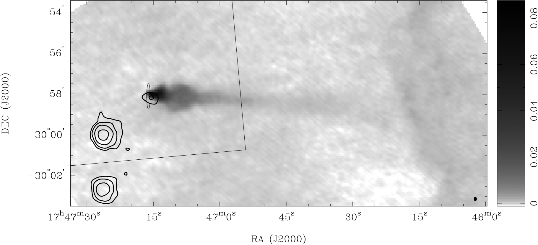
Figure 1.— Existing radio and X-ray data on G359.23–0.82 (“the Mouse”) and PSR J1747–2958. The image shows a Very Large Array (VLA) image at a frequency of 1.5 GHz. The brightness scale is logarithmic, ranging between –1.3 and 87.6 mJy beam^-1 as shown by the scale bar to the right of the image. This image is made from VLA observations in the CnB and DnC configurations, carried out on 1986 Oct 11/12 and 1987 Feb 20, respectively. The spatial resolution is $12\farcs 8\times 8\farcs 4$, as shown by the filled ellipse in the lower right corner of the image. The original 1-$\sigma$ error ellipse on the position of PSR J1747–2958, as reported by Camilo et al. (2002), is shown at the head of the radio nebula. Also overlaid are contours from a ROSAT PSPC observation carried out on 1992 Mar 02 of duration 2000 s, convolved with a gaussian of dimensions $20^{\prime\prime}\times 20^{\prime\prime}$. Contour levels are drawn at levels of 4%, 8%, 20% and 60% of the peak. The two straight lines indicate the southern and western edges of the Chandra ACIS-S3 field of view.

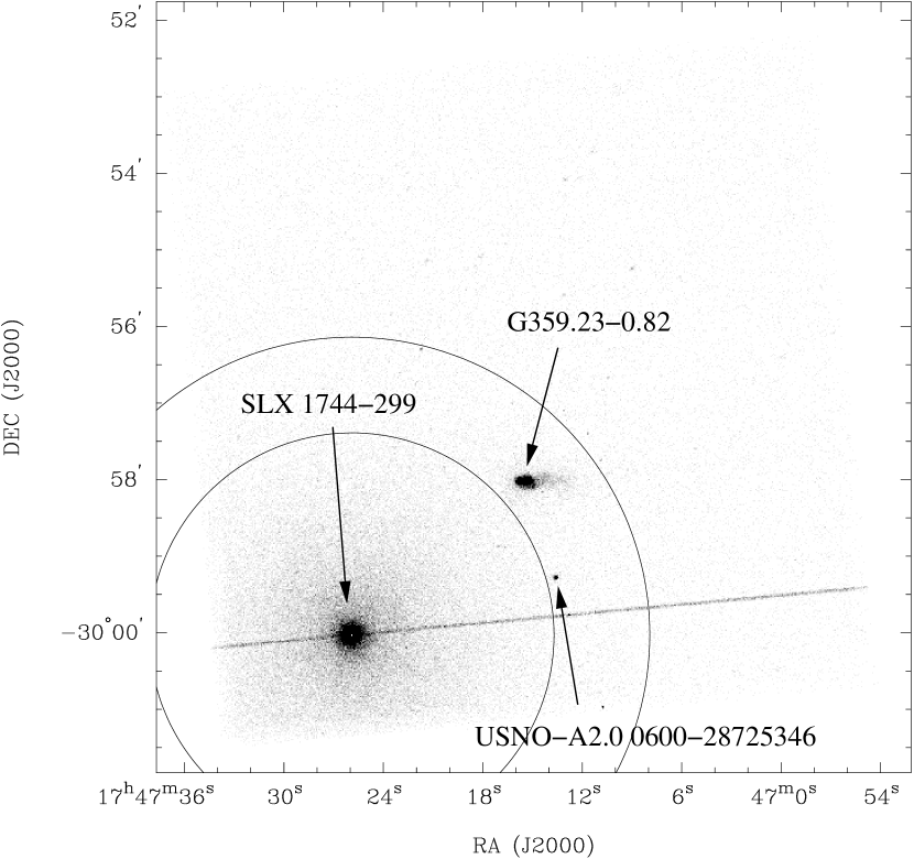
Figure 2.— Chandra image of the ACIS-S3 field of view in the energy range 0.5 to 8.0 keV. This image has not been corrected for spatially-varying exposure across the field of view. Sources discussed in the text are labeled. The region lying between the two circles (but excluding G359.23–0.82, the USNO-A2.0 star 0600-28725346 and the read-out streak from SLX 1744–299) was used to estimate the background level when carrying out spectroscopy of G359.23–0.82.

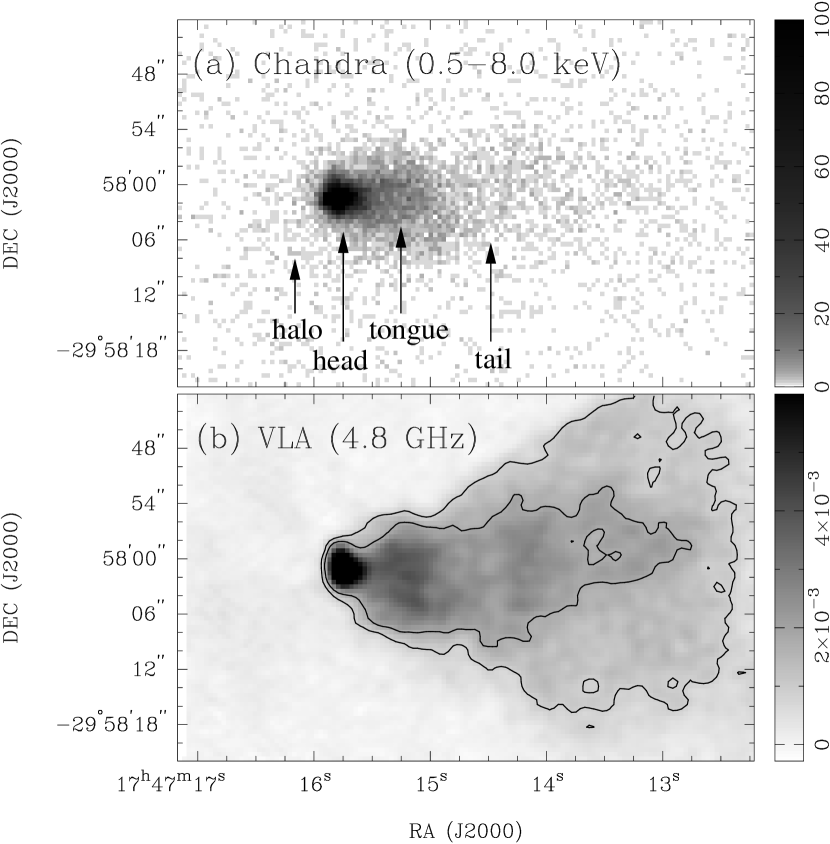
Figure 3.— X-ray and radio images of the Mouse. (a) Chandra image of the Mouse in the energy range 0.5–8.0 keV. The brightness scale is logarithmic, ranging between 0 and 100 counts, as shown by the scale bar to the right of the image. Various features discussed in the text are indicated. This image has not been exposure corrected. (b) VLA image of the Mouse at a frequency of 4.8 GHz. The brightness scale is linear, ranging between –0.2 and 6.0 mJy beam^-1 as shown by the scale bar to the right of the image. The contours are at levels of 0.9 and 1.8 mJy beam^-1, chosen to highlight the two different components seen in the radio “tail”. This image is made from VLA observations in BnA and CnB arrays, carried out on 1987 Nov 07 and 1988 Feb 25, respectively, with a resulting spatial resolution of $1\farcs 6\times 1\farcs 7$.

Figure 4.— 0.5–8.0 keV brightness profile of G359.23–0.82 in the east-west direction (negative offsets are to the east). The solid line and data points represent the X-ray surface brightness of G359.23–0.82 as a function of offset from the peak, averaged over a column of nine $0\farcs 492\times 0\farcs 492$ pixels bisected by the symmetry axis of the source. The dashed line indicates the brightness of the background, determined by averaging a column of 121 pixels immediately to the north and south of G359.23–0.82. The dot-dashed line divides the logarithmic scale in the upper panel from the linear scale in the lower panel. Various features discussed in the text are indicated.

Figure 5.— Radio and X-ray brightness profiles of the “tail” of G359.23–0.82 in the north-south direction (negative offsets are to the south). The solid line represents the X-ray surface brightness of the tail as a function of offset from the symmetry axis, averaged over a row of 26 $0\farcs 492\times 0\farcs 492$ pixels centered on RA (J2000) $17^{\rm h}47^{\rm m}13\fs 8$. The dashed line indicates the radio surface brightness of the tail as a function of offset from the symmetry axis at RA (J2000) $17^{\rm h}47^{\rm m}13\fs 4$. Both profiles have been Hanning smoothed with a smoothing length of five ACIS pixels, or $2\farcs 46$. The narrow component of the tail is seen in both radio and X-rays, while the broad component appears only in the radio.

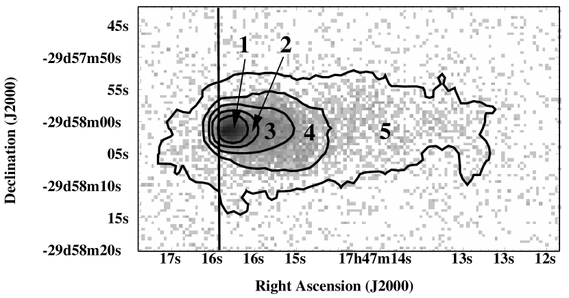
Figure 6.— Image as in Fig. 3(a), but showing the extraction regions used for spectroscopy. The five regions indicated are mutually exclusive, each lying between successive sets of contours, but consisting only of data lying to the west of the vertical line. Region 6 is not shown, but consists of all points to the east of this line which fall within an annulus centered on the peak, of inner radius $4\farcs 8$ and outer radius $14\farcs 1$.

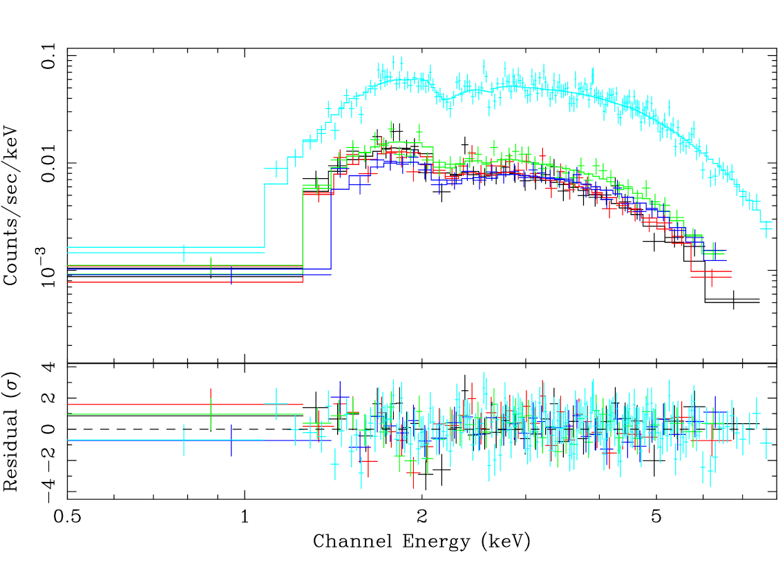
Figure 7.— Chandra spectrum of G359.23–0.82 in the five different regions shown in Fig. 6. The points in the upper panel indicate the data in each region, while the solid lines show the corresponding best fit power law models, resulting from fits to the data in which all regions are constrained to have the same value of $N_{H}$. The spectrum for region 1 (top curve, shown in light blue in the electronic edition) includes the effect of pile-up.

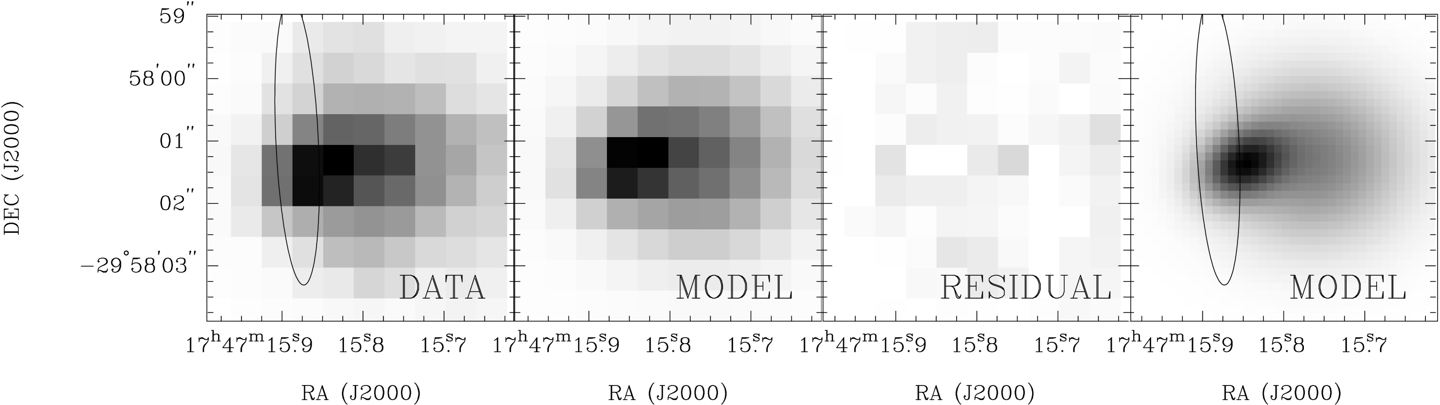
Figure 8.— Spatial structure in the brightest regions of G359.23–0.82. The leftmost panel shows the 0.5–8.0 keV image of G359.23–0.82 in the immediate vicinity of the peak of X-ray emission; individual $0\farcs 49\times 0\farcs 49$ ACIS pixels can be seen. The transfer function in this image is linear, ranging between 0 and 350 counts per ACIS pixel. The center left panel shows a fit to these data, using a model consisting of two gaussians plus a constant offset (see §3.4 and Table 2 for details); the transfer function and greyscale range are the same as in the leftmost panel. The center right panel shows the residual between the data and the model, again using the same transfer function and greyscale range. The rightmost panel shows the model again, but this time resampled using $0\farcs 12\times 0\farcs 12$ pixels, and using a linear greyscale ranging between 0.2 and 27.3 counts per $0\farcs 12\times 0\farcs 12$ pixel. In the first and fourth panels, the ellipse shows our revised 3-$\sigma$ confidence limits on the position of PSR J1747–2958, as determined by the radio timing results presented in §3.5 and in Table 3.

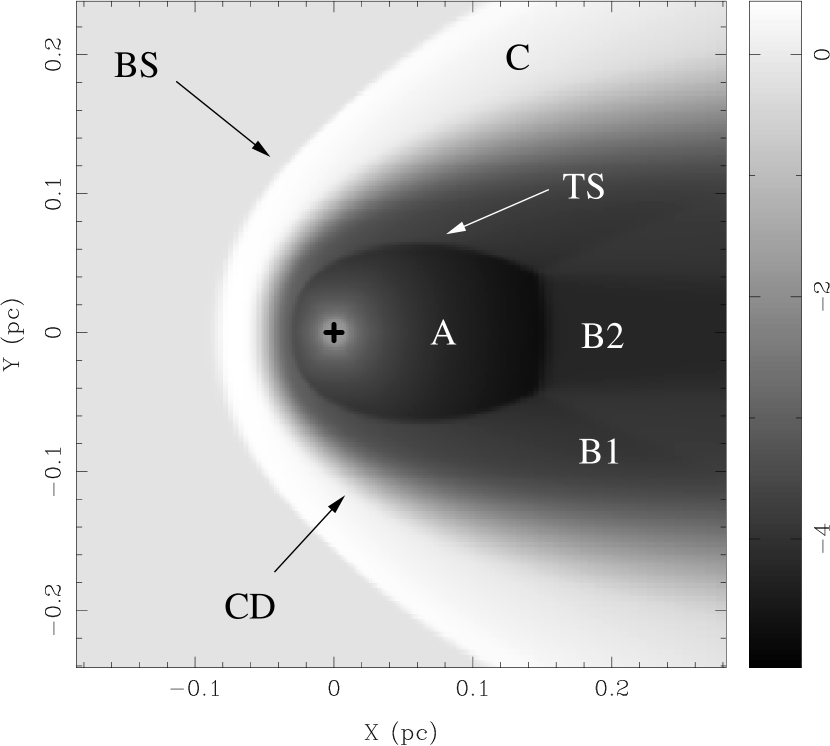
Figure 9.— Axially symmetric hydrodynamic simulation of a bow shock, generated by a pulsar with an isotropic wind moving from right to left through a homogeneous ambient medium. The position of the pulsar is indicated by the “+” symbol; regions referred to in the text are indicated. Simulation parameters for the pulsar and ambient medium are as described in §4.3. The greyscale is on a logarithmic scale; the units in the scale bar are $\log_{10}\rho$, where $\rho$ is the ambient mass density in units of $10^{-24}$ g cm^-3.

References

- Arons (2002) Arons, J. 2002, in Neutron Stars in Supernova Remnants, ed. P. O. Slane & B. M. Gaensler (San Francisco: Astronomical Society of the Pacific), 71–80
- Arons & Tavani (1993) Arons, J. & Tavani, M. 1993, ApJ, 403, 249
- Arzoumanian et al. (2002) Arzoumanian, Z., Chernoff, D. F., & Cordes, J. M. 2002, ApJ, 568, 289
- Arzoumanian et al. (1994) Arzoumanian, Z., Nice, D. J., Taylor, J. H., & Thorsett, S. E. 1994, ApJ, 422, 671
- Bamba et al. (2000) Bamba, A., Yokogawa, J., Sakano, M., & Koyama, K. 2000, PASJ, 52, 259
- Bałucińska-Church & McCammon (1992) Bałucińska-Church, M. & McCammon, D. 1992, ApJ, 400, 699
- Bavassano et al. (1974) Bavassano, B., Mariana, F., & Villante, U. 1974, Space Res., 14, 403
- Bietenholz et al. (2001) Bietenholz, M. F., Frail, D. A., & Hester, J. J. 2001, ApJ, 560, 254
- Braje et al. (2002) Braje, T. M., Romani, R. W., Roberts, M. S. E., & Kawai, N. 2002, ApJ, 565, L91
- Braun et al. (1989) Braun, R., Goss, W. M., & Lyne, A. G. 1989, ApJ, 340, 355
- Bronfman et al. (1988) Bronfman, L., Cohen, R. S., Alvarez, H., May, J., & Thaddeus, P. 1988, ApJ, 324, 248
- Bucciantini (2002) Bucciantini, N. 2002, A&A, 387, 1066
- Bucciantini & Bandiera (2001) Bucciantini, N. & Bandiera, R. 2001, A&A, 375, 1032
- Burke et al. (1997) Burke, B. E., Gregory, J., Bautz, M. W., Prigozhin, G. Y., Kissel, S. E., Kosicki, B. N., Loomis, A. H., & Young, D. J. 1997, IEEE Transac. Elec. Devices, 44, 1633
- Camilo et al. (2001) Camilo, F., Bell, J. F., Manchester, R. N., Lyne, A. G., Possenti, A., Kramer, M., Kaspi, V. M., Stairs, I. H., D’Amico, N., Hobbs, G., Gotthelf, E. V., & Gaensler, B. M. 2001, ApJ, 557, L51
- Camilo et al. (2002) Camilo, F., Manchester, R. N., Gaensler, B. M., & Lorimer, D. R. 2002, ApJ, 579, L25
- Caraveo et al. (2003) Caraveo, P. A., Bignami, G. F., DeLuca, A., Mereghetti, S., Pellizzoni, A., Mignani, R., Tur, A., & Becker, W. 2003, Science, 301, 1345
- Chatterjee & Cordes (2004) Chatterjee, S. & Cordes, J. M. 2004, ApJ, 600, L51
- Chatterjee & Cordes (2002) Chatterjee, S. & Cordes, J, M. 2002, ApJ, 575, 407
- Chen et al. (1996) Chen, Y., Bandiera, R., & Wang, Z.-R. 1996, ApJ, 469, 715
- Chevalier (2000) Chevalier, R. A. 2000, ApJ, 539, L45
- Clemens et al. (1988) Clemens, D. P., Sanders, D. B., & Scoville, N. Z. 1988, ApJ, 327, 139
- Comerón & Kaper (1998) Comerón, F. & Kaper, L. 1998, A&A, 338, 273
- Cordes (1996) Cordes, J. M. 1996, in Pulsars: Problems and Progress, IAU Colloquium 160, ed. S. Johnston, M. A. Walker, & M. Bailes (San Francisco: Astronomical Society of the Pacific), 393–399
- Cordes & Lazio (2002) Cordes, J. M. & Lazio, T. J. W. 2002, preprint (astro-ph/0207156)
- Dame (1993) Dame, T. M. 1993, in Back to the Galaxy, ed. S. S. Holt & F. Verter, Vol. 278 (New York: AIP), 267–278
- Davis (2001) Davis, J. E. 2001, ApJ, 562, 575
- Dib & Kaspi (2004) Dib, R. & Kaspi, V. M. 2004, in preparation
- Ferrière (2001) Ferrière, K. M. 2001, Reviews of Modern Physics, 73, 1031
- Frail et al. (1996) Frail, D. A., Giacani, E. B., Goss, W. M., & Dubner, G. 1996, ApJ, 464, L165
- Freeman et al. (2002) Freeman, P. E., Kashyap, V., Rosner, R., & Lamb, D. Q. 2002, ApJ, 138, 185
- Gaensler (2004) Gaensler, B. M. 2004, in Young Neutron Stars and their Environments, ed. F. Camilo & B. M. Gaensler (San Francisco: Astronomical Society of the Pacific), 151–158
- Gaensler et al. (2002a) Gaensler, B. M., Arons, J., Kaspi, V. M., Pivovaroff, M. J., Kawai, N., & Tamura, K. 2002a, ApJ, 569, 878
- Gaensler & Frail (2000) Gaensler, B. M. & Frail, D. A. 2000, Nature, 406, 158
- Gaensler et al. (2002b) Gaensler, B. M., Jones, D. H., & Stappers, B. W. 2002b, ApJ, 580, L137
- Gaensler et al. (2003) Gaensler, B. M., Schulz, N. S., Kaspi, V. M., Pivovaroff, M. J., & Becker, W. E. 2003, ApJ, 588, 441
- Gaensler et al. (2004) Gaensler, B. M., Stappers, B., Chatterjee, S., Ghavamian, P., Jones, D. H., & Cordes, J. 2004, in How Does the Galaxy work?, ed. E. J. Alfaro, E. Pérez, & J. Franco (Dordrecht: Kluwer), in press (astro-ph/0309740)
- Gallant & Arons (1994) Gallant, Y. A. & Arons, J. 1994, ApJ, 435, 230
- Gavriil et al. (2004) Gavriil, F. P., Kaspi, V. M., & Roberts, M. S. E. 2004, Adv. Space Res., 33, 592
- Gotthelf (2003) Gotthelf, E. V. 2003, ApJ, 591, 361
- Gotthelf (2004) Gotthelf, E. V. 2004, in Young Neutron Stars and their Environments, ed. F. Camilo & B. M. Gaensler (San Francisco: Astronomical Society of the Pacific), 225–228
- Gvaramadze (2004) Gvaramadze, V. V. 2004, A&A, 415, 1073
- Harrus et al. (1997) Harrus, I. M., Hughes, J. P., Singh, K. P., Koyama, K., & Asaoka, I. 1997, ApJ, 488, 781
- Heiles (2001) Heiles, C. 2001, in Tetons 4: Galactic Structure, Stars and the Interstellar Medium, ed. C. E. Woodward, M. D. Bicay, & J. M. Shull, Vol. 231 (San Francisco: ASP), 294
- Helfand et al. (2001) Helfand, D. J., Gotthelf, E. V., & Halpern, J. P. 2001, ApJ, 556, 380
- Hester et al. (1995) Hester, J. J., Scowen, P. A., Sankrit, R., Burrows, C. J., Gallagher, III, J. S., Holtzman, J. A., Watson, A., Trauger, J. T., Ballester, G. E., Casertano, S., Clarke, J. T., Crisp, D., Evans, R. W., Griffiths, R. E., Hoessel, J. G., Krist, J., Lynds, R., Mould, J. R., O’Neill, Jr., E. J., Stapelfeldt, K. R., & Westphal, J. A. 1995, ApJ, 448, 240
- Hoshino et al. (1992) Hoshino, M., Arons, J., Gallant, Y. A., & Langdon, A. B. 1992, ApJ, 390, 454
- Hughes et al. (2003) Hughes, J. P., Slane, P. O., Park, S., Roming, P. W. A., & Burrows, D. N. 2003, ApJ, 591, L139
- Johnston et al. (2001) Johnston, S., Koribalski, B., Weisberg, J. M., & Wilson, W. 2001, MNRAS, 322, 715
- Jones et al. (2002) Jones, D. H., Stappers, B. W., & Gaensler, B. M. 2002, A&A, 389, L1
- Kafatos et al. (1980) Kafatos, M., Sofia, S., Bruhweiler, F., & Gull, S. 1980, ApJ, 242, 294
- Kaspi et al. (2001) Kaspi, V. M., Gotthelf, E. V., Gaensler, B. M., & Lyutikov, M. 2001, ApJ, 562, L163
- Kennel & Coroniti (1984a) Kennel, C. F. & Coroniti, F. V. 1984a, ApJ, 283, 694
- Kennel & Coroniti (1984b) —. 1984b, ApJ, 283, 710
- Komissarov & Lyubarsky (2003) Komissarov, S. S. & Lyubarsky, Y. E. 2003, MNRAS, 344, L93
- Li et al. (2003) Li, J., Kastner, J. H., Prigozhin, G. Y., & Schulz, N. S. 2003, ApJ, 590, 586
- Linde et al. (1998) Linde, T. J., Gombosi, T. I., Roe, P. L., Powell, K. G., & DeZeeuw, D. L. 1998, J. Geophys. Res., 103, 1889
- Lou (1998) Lou, Y.-Q. 1998, MNRAS, 294, 443
- Lu et al. (2002) Lu, F. J., Wang, Q. D., Aschenbach, B., Durouchoux, P., & Song, L. M. 2002, ApJ, 568, L49
- Lyne et al. (1996) Lyne, A. G., Pritchard, R. S., Graham-Smith, F., & Camilo, F. 1996, Nature, 381, 497
- Lyutikov (2003) Lyutikov, M. 2003, MNRAS, 339, 623
- Lyutikov (2004) —. 2004, in preparation
- Mac Low et al. (1991) Mac Low, M.-M., van Buren, D., Wood, D. O. S., & Churchwell, E. 1991, ApJ, 369, 395
- Manchester et al. (1991) Manchester, R. N., Kaspi, V. M., Johnston, S., Lyne, A. G., & D’Amico, N. 1991, MNRAS, 253, 7P
- Mathis & Lee (1991) Mathis, J. S. & Lee, C.-W. 1991, ApJ, 376, 490
- Monet et al. (1998) Monet, D., Bird, A., Canzian, B., Dahn, C., Guetter, H., Harris, H., Henden, A., Levine, S., Luginbuhl, C., Monet, A. K. B., Rhodes, A., Riepe, B., Sell, S., Stone, R., Vrba, F., & R., W. 1998, USNO-A V2.0, A Catalog of Astrometric Standards (Washington DC: US Naval Observatory)
- Moon et al. (2004) Moon, D.-S., Lee, J.-J., Eikenberry, S. S., Koo, B.-C., Chatterjee, S., L., K. D., Hester, J. J., Cordes, J. M., Gallant, Y. A., & Koch-Miramond, L. 2004, ApJ, 610, L33
- Ng & Romani (2004) Ng, C.-Y. & Romani, R. W. 2004, ApJ, 601, 479
- Olbert et al. (2001) Olbert, C. M., Clearfield, C. R., Williams, N. E., Keohane, J. W., & Frail, D. A. 2001, ApJ, 554, L205
- Olbert et al. (2003) Olbert, C. M., Keohane, J. W., Arnaud, K. A., Dyer, K. K., Reynolds, S. P., & Safi-Harb, S. 2003, ApJ, 592, L45
- Pavlov et al. (2003) Pavlov, G. G., Teter, M. A., Kargaltsev, O., & Sanwal, D. 2003, ApJ, 591, 1157
- Pelling et al. (1987) Pelling, R. M., Paciesas, W. S., Peterson, L. E., Makishima, K., Oda, M., Ogawara, Y., & Miyamoto, S. 1987, ApJ, 319, 416
- Petre et al. (2002) Petre, R., Kuntz, K. D., & Shelton, R. L. 2002, ApJ, 579, 404
- Possenti et al. (2002) Possenti, A., Cerutti, R., Colpi, M., & Mereghetti, S. 2002, A&A, 387, 993
- Predehl & Kulkarni (1995) Predehl, P. & Kulkarni, S. R. 1995, A&A, 294, L29
- Raymond & Smith (1977) Raymond, J. C. & Smith, B. W. 1977, ApJS, 35, 419
- Rees & Gunn (1974) Rees, M. J. & Gunn, J. E. 1974, MNRAS, 167, 1
- Rho et al. (1994) Rho, J., Petre, R., Schlegel, E., & Hester, J. 1994, ApJ, 430, 757
- Roberts et al. (2003) Roberts, M. S. E., Tam, C. R., Kaspi, V. M., Lyutikov, M., Vasisht, G., Pivovaroff, M., Gotthelf, E. V., & Kawai, N. 2003, ApJ, 588, 992
- Seta et al. (2004) Seta, M., Hasegawa, T., Sakomoto, S., Oka, T., Sawada, T., Inutsuka, S., Koyama, H., & Hayashi, M. 2004, AJ, 127, 1098
- Shull et al. (1989) Shull, J. M., Fesen, R. A., & Saken, J. M. 1989, ApJ, 346, 860
- Sidoli et al. (2001) Sidoli, L., Belloni, T., & Mereghetti, S. 2001, A&A, 368, 835
- Sidoli et al. (1999) Sidoli, L., Mereghetti, S., Israel, G. L., Chiappetti, L., Treves, A., & Orlandini, M. 1999, ApJ, 525, 215
- Skinner et al. (1987) Skinner, G. K., Willmore, A. P., Eyles, C. J., Bertram, D., & Church, M. J. 1987, Nature, 330, 544
- Slane et al. (2000) Slane, P., Chen, Y., Schulz, N. S., Seward, F. D., Hughes, J. P., & Gaensler, B. M. 2000, ApJ, 533, L29
- Slavin et al. (1983) Slavin, J. E., Tsurutani, B. T., Smith, E. J., Jones, D. E., & Sibeck, D. G. 1983, Geophys. Res. Lett., 10, 973
- Stappers et al. (2003) Stappers, B. W., Gaensler, B. M., Kaspi, V. M., van der Klis, M., & Lewin, W. H. G. 2003, Science, 299, 1372
- Taylor & Cordes (1993) Taylor, J. H. & Cordes, J. M. 1993, ApJ, 411, 674
- Toropina et al. (2001) Toropina, O. D., Romanova, M. M., Toropin, Y. M., & Lovelace, R. V. E. 2001, ApJ, 561, 964
- Tóth (1996) Tóth, G. 1996, Astrophys. Let. Comm., 34, 245
- Townsley et al. (2002) Townsley, L. K., Broos, P. S., Chartas, G., Moskalenko, E., Nousek, J. A., & Pavlov, G. G. 2002, Nucl. Instr. & Methods in Phys. Res. A, 486, 716
- Uchida et al. (1992) Uchida, K., Morris, M., & Yusef-Zadeh, F. 1992, AJ, 104, 1533
- van Buren (1993) van Buren, D. 1993, in Massive stars: Their lives in the interstellar medium, ed. J. P. Cassinelli & E. B. Churchwell (San Francisco: Astronomical Society of the Pacific), 315–326
- van Buren & McCray (1988) van Buren, D. & McCray, R. 1988, ApJ, 329, L93
- van der Swaluw (2004) van der Swaluw, E. 2004, Adv. Space Res., 33
- van der Swaluw et al. (2003) van der Swaluw, E., Achterberg, A., Gallant, Y. A., Downes, T. P., & Keppens, R. 2003, A&A, 397, 913
- van der Swaluw et al. (2004) van der Swaluw, E., Downes, T. P., & Keegan, R. 2004, A&A, 420, 937
- van Kerkwijk & Kulkarni (2001) van Kerkwijk, M. H. & Kulkarni, S. R. 2001, A&A, 380, 221
- Wang et al. (2002) Wang, Q. D., Lu, F., & Lang, C. C. 2002, ApJ, 581, 1148
- Weisskopf et al. (2000) Weisskopf, M. C., Hester, J. J., Tennant, A. F., Elsner, R. F., Schulz, N. S., Marshall, H. L., Karovska, M., Nichols, J. S., Swartz, D. A., Kolodziejczak, J. J., & O’Dell, S. L. 2000, ApJ, 536, L81
- Wilkin (1996) Wilkin, F. P. 1996, ApJ, 459, L31
- Wolszczan et al. (1991) Wolszczan, A., Cordes, J. M., & Dewey, R. J. 1991, ApJ, 372, L99
- Wong et al. (2002) Wong, D. S., Cordes, J. M., Chatterjee, S., Zweibel, E., Finley, J., Romani, R., & Ulmer, M. 2002, AAS HEAD, N17.120
- Yusef-Zadeh & Bally (1987) Yusef-Zadeh, F. & Bally, J. 1987, Nature, 330, 455
- Yusef-Zadeh & Bally (1989) Yusef-Zadeh, F. & Bally, J. 1989, in The Center of the Galaxy (IAU Symp. 136), ed. M. Morris (Dordrecht: Kluwer), 197–204
- Zank (1999) Zank, G. P. 1999, Space Sci. Rev., 89, 413