The MUNICS Project: Galaxy Assembly at $0<z<1$

The MUNICS Project: Galaxy Assembly at $0<z<1$

1 The MUNICS Survey and its Results

MUNICS is a wide-area, medium-deep, photometric and spectroscopic survey selected in the K band, targeting randomly-selected high Galactic latitude fields. It covers an area of roughly one square degree in the K and J bands with complementary optical follow-up imaging in the I, R, V, and B bands in 0.5 square degrees.

The limiting magnitudes of this main part of the survey are 19.5 in K, 21.5 in J, 22.5 in I, and 23.5 in R (50 % completeness for point-like sources). This multicolor catalog probes field galaxies in a large volume out to redshifts of roughly 1.5 (for massive galaxies) and is by far the largest catalog of near-infrared selected distant galaxies published so far. It thus comprises a suitable and highly competitive multi-color field galaxy survey. The photometric survey is described and characterized in MUNICS1 and MUNICS4 . The survey spans the redshift range $0<z<1.5$ and selects typically $L^{*}$ and brighter objects.

The MUNICS photometric survey is complemented by spectroscopic follow-up observations at 4m-class telescopes of all galaxies down to $K\leq 17.5$ in 0.25 square degrees. This survey is complete down to $K\leq 16.5$ and 80% complete at $16.5<K<17.5$ to the present date. Furthermore, a sparsely selected deeper sample down to $K\leq 19$ was observed with the ESO VLT, covering a much smaller area of 100 square arcmin. The whole spectroscopic sample contains 593 secured redshifts thsu far. The spectra cover a wide wavelength range $4000-8500$Å at $13.2$Å resolution, and sample galaxies at $0<z<1$. Details of the spectroscopic survey are given in MUNICS5 .

Since it is impossible to obtain spectroscopic redshifts for the whole MUNICS sample (most galaxies in the sample are too faint to be observed currently with optical spectrographs) one must rely on photometric redshift techniques to obtain distance estimates for the complete sample of almost 6000 galaxies. Comparing to $>500$ spectroscopic redshifts, the scatter in the relative redshift error $\Delta z/(1+z)$ is 0.055. The distribution of photometric redshifts peaks around $z\approx 0.5$. and has a tail extending to $z\approx 3$.

Given these limits, MUNICS contains mostly massive (stellar mass $M>10^{10}M_{\odot}$) field galaxies, spanning a significant fraction of cosmic time and is ideal for studying their formation and evolution, specifically their mass assembly history.

2 The Rest-frame K-Band Luminosity Function to $\bf z\sim 1.2$

Fig. 1 shows the rest-frame K–band luminosity function (LF) derived from the MUNICS data in four redshift bins spanning $0.4<z<1.2$ MUNICS2 . Absolute magnitudes were derived using the photometric redshifts, extrapolating the best fitting SED to the rest-frame K band. Errors due to this extrapolation are expected to be small in the redshift range we probe, since the near-IR slopes of the SEDs differ only very little over the galaxy types probed by our survey (the K–band $k$-corrections are small and almost type-independent).

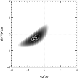
Figure 1: Left panel: The rest-frame K–band luminosity function derived from the MUNICS data in four redshift bins spanning $0.4<z<1.2$. The dotted curve is the $z=0$ LF Kochaneketal01 . The dashed lines are parameterized fits to the data. Right panel: Likelihood map for the change in the Schechter parameters, $d\Phi^{*}/(\Phi^{*}\,dz)$ and $dM^{*}/dz$, with redshift.

Quantitative analysis of the evolution of the LF yields a mild decrease in number density by $\sim 25\%$ to $z=1$ accompanied by brightening of the galaxy population by $\sim 0.5$ mag. These results are fully consistent with an analogous analysis using only the spectroscopic MUNICS sample MUNICS5 , which is shown in Fig. 2.

Figure 2: The K band luminosity function of galaxies from spectroscopic observations of MUNICS galaxies. The dotted and dashed curves are the $z=0$ LFs Loveday00 ; Kochaneketal01 .

To interpret these results in terms of a picture of galaxy evolution is not straight–forward, though. Since the K–band light traces stellar mass, we may attribute a change in K band luminosity function either to a change in the mass–to–light ratio alone (passive evolution) or to a combination of a change in $M/L$ and in stellar mass. A change in stellar mass can be due to star formation and/or due to merging and accretion. These models cannot be discriminated on basis of the luminosity function alone. In fact, if the increase seen in the global star formation rate to $z\sim 1$ (e.g. CFRS96 ; CFRS1297 ; HCBP98 ; CSB99 ) is attributable to normal field galaxies, the stellar mass of these systems is expected to evolve by roughly a factor of 1.5 to 2 over the redshift range $0<z<1$. Therefore, if the K band light does reflect stellar mass, number density evolution in the K band is indeed expected.

3 The Stellar Mass of Field Galaxies to $\bf z\sim 1.2$

The multicolor data in MUNICS with their wide range in wavelength allow us to investigate properties of the stellar populations of individual objects in greater detail. We can therefore use the MUNICS data to derive the stellar mass function in the redshift range $0.4<z<1.2$ MUNICS6 ; MUNICS3 by modeling and fitting the stellar mass-to-light ratios in the NIR.

We parameterize star formation histories as $\psi(t)\propto\exp(-t/\tau)$, with $\tau\in\{0.1,0.2,0.4,1.0,2.0,3.0,5.0,8.0,10.0,13.0\}$ Gyr. We extract spectra at 28 ages between 0.001 and 14 Gyr and allow $A_{v}$ to vary between 0 and 3 mag using a Calzetti Calzetti00 extinction law. The models use solar metallicity and are based on the Simple Stellar Population models by C. Maraston Maraston98 . We assume a value of 3.33 for the absolute K–band magnitude of the Sun. We use a Salpeter IMF with lower and upper mass cutoffs of 0.1 and 100 $M_{\odot}$. This choice allows us to compare our results directly with the literature. The use of an IMF with a flatter slope at the low mass end will not affect the shape of the mass function, it will only change its overall normalization. If, however, the IMF depends on the mode of star formation, e.g. being top–heavy in starbursts, our results will be affected. We convert the absolute K–band magnitude, $M_{K}$, into stellar mass by using the K–band mass–to–light ratio, $M/L_{K}$, of the best fitting CSP model in a $\chi^{2}$ sense.

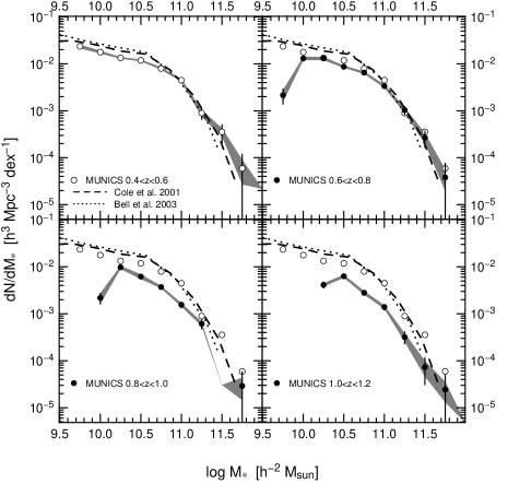
Figure 3: The evolution of the stellar mass function with redshift. The open symbols are the MUNICS values at $0.4<z<0.6$, the closed symbols are the MUNICS values at higher redshifts. The lowest $z$ values are shown in all panels for comparison. Error bars denote the uncertainty due to Poisson statistics. The shaded areas show the 1 $\sigma$ range of variation in the mass function given the total systematic uncertainty in $M/L_{K}$. The dotted and dashed lines show the $z=0$ stellar mass function derived similarly to our methods using SDSS, 2dF, and 2MASS data BMKW03 ; 2dF01 .

Fig. 3 shows the mass function of galaxies with $10^{10}<M/(h^{-2}\,M_{\odot})<10^{12}$ in four redshift bins centered at $z=0.5$, $z=0.7$, $z=0.9$, and $z=1.1$. The results on the local stellar mass function 2dF01 ; BMKW03 derived by fitting stellar population models to multicolor photometry and deriving NIR mass–to–light ratios similarly to the method employed here are also shown for comparison as a dashed and dotted line, respectively. The data from the lowest redshift bin, $0.4<z<0.6$ are shown alongside the higher–redshift data for easier comparison as open symbols. Error bars denote the uncertainty due to Poisson statistics. The shaded areas show the 1 $\sigma$ range of variation in the mass function from Monte–Carlo simulations given our estimate of the total systematic uncertainty in $M/L_{K}$.

The lowest redshift bin shows remarkable agreement with the $z=0$ values, despite the different selection at low versus high redshift and the different model grids used, although we obtain slightly lower number densities at $\log M/(h^{-2}\,M_{\odot})\leq 10.5$. Therefore, there seems to be not much evolution in stellar mass at $z<0.5$. The general trend at higher redshift, is for the total normalization of the stellar mass function to goes down and for the knee to move towards lower masses. This causes the higher masses to evolve faster in number density than lower masses and is well visible in Fig. 3 at $10.5<\log M/(h^{-2}\,M_{\odot})<11.5$.

4 The total stellar mass density

The total stellar mass density of the universe – the integral of the star formation history of the universe (e.g. Madauetal96 ; SAGDP99 ) and observationally its complement – is shown in Fig. 4. We also plot the local value from 2dF01 , values from the Hubble Deep Fields DPFB03 ; Fontanaetal03 covering $z>1$ and values from Cohen02 ; BE00 at $z<1$. Additionally, we integrate the star formation history curve (including extinction correction) from SAGDP99 for comparison.

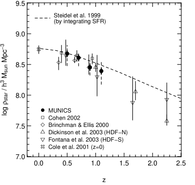
Figure 4: The evolution of the total stellar mass density in the universe. The closed circles are the MUNICS values, open symbols are values from the literature. The integrated star formation rate (dashed curve) is shown for comparison. The thick error bars on the MUNICS values (solid dots) are the statistical errors associated with the data. The dashed error bars show the variance we get from the MUNICS data in GOODS size patches.

From our data, as well as from the HDFs and the integrated star formation rate from the UV luminosity density, it appears that 50% of the local mass in stars has formed since $z\sim 1$. The data from BE00 are consistent with ours at $z\sim 1$ but are lower at $z\sim 0.4$ and seem to under–predict the local value if extrapolated. The values obtained by Cohen02 are higher at $z\sim 1$ which we think is attributable to their method of deriving $M/L_{K}$.

It is worth noting that the results from the HDF–N differ by a factor $\sim 2$ from the HDF–S, attributable to cosmic variance. The MUNICS values in Fig. 4 are shown with their statistical errors (thick error bars), which amount to roughly 10%. We also show the variance we get in our sample divided into GOODS size patches of 150 square arcminutes (dashed error bars), showing that at these redshifts, even surveys like GOODS are expected to be dominated by cosmic variance. We expect differences of around 50% between the two GOODS areas.

References

- (1) Bell, E. F., McIntosh, D. H., Katz, N., & Weinberg, M. D. 2003, ApJ, submitted
- (2) Brinchmann, J., & Ellis, R. S. 2000, ApJ, 536, L77
- (3) Calzetti, D., Armus, L., Bohlin, R. C., Kinney, A. L., Koornneef, J., & Storchi-Bergmann, T. 2000, ApJ, 533, 682
- (4) Cohen, J. G. 2002, ApJ, 567, 672
- (5) Cole, S., et al. 2001, MNRAS, 326, 255
- (6) Cowie, L. L., Songaila, A., & Barger, A. J. 1999, AJ, 118, 603
- (7) Dickinson, M., Papovich, C., Ferguson, H. C., & Budavári, T. 2003, ApJ, 587, 25
- (8) Drory, N., Bender, R., Feulner, G., Hopp, U., Maraston, C., Snigula, J., & Hill, G. J. 2003a, ApJ, 595, 698
- (9) Drory, N., Bender, R., Feulner, G., Hopp, U., Maraston, C., Snigula, J., & Hill, G. J. 2003b, ApJ, submitted
- (10) Drory, N., Bender, R., Snigula, J., Feulner, G., Hopp, U., Maraston, C., Hill, G. J., & de Oliveira, C. M. 2001a, ApJ, 562, L111
- (11) Drory, N., Feulner, G., Bender, R., Botzler, C. S., Hopp, U., Maraston, C., Mendes de Oliveira, C., & Snigula, J. 2001b, MNRAS, 325, 550
- (12) Feulner, G., Bender, R., Drory, N., Hopp, U., Snigula, J., & Hill, G. J. 2003, MNRAS, 342, 605
- (13) Fontana, A., et al. 2003, ApJ, 594, L9
- (14) Hammer, F., et al. 1997, ApJ, 481, 49
- (15) Hogg, D. W., Cohen, J. G., Blandford, R., & Pahre, M. A. 1998, ApJ, 504, 622
- (16) Kochanek, C. S., et al. 2001, ApJ, 560, 566
- (17) Lilly, S. J., Le Fèvre, O., Hammer, F., & Crampton, D. 1996, ApJ, 460, L1
- (18) Loveday, J. 2000, MNRAS, 312, 557
- (19) Madau, P., Ferguson, H. C., Dickinson, M. E., Giavalisco, M., Steidel, C. C., & Fruchter, A. 1996, MNRAS, 283, 1388
- (20) Maraston, C. 1998, MNRAS, 300, 872
- (21) Snigula, J., Drory, N., Bender, R., Botzler, C. S., Feulner, G., & Hopp, U. 2002, MNRAS, 336, 1329
- (22) Steidel, C. C., Adelberger, K. L., Giavalisco, M., Dickinson, M., & Pettini, M. 1999, ApJ, 519, 1