On the evolution of the cosmic-mass-density contrast and the cosmological constant

We study the evolution of the cosmic mass density contrast beyond the Robertson-Walker geometry including the small contribution of acceleration. We derive a second-order evolution equation for the density contrast within the spherical model for CDM collissionless fluid including the cosmological constant, the expansion and the non-vanishing four-vector of acceleration. While the mass-density is not seriously affected by acceleration, the mass-density contrast changes its shape at smaller redshifts even for a small amount of the acceleration parameter. This could help to resolve current controversial results in cosmology from measurements of WMAP, gravitational lensing, XMM X-ray cluster or type Ia supernovae data, etc.

1 Motivation

With more and more precise measurements in cosmology, theorists are confronted with more and more questions with no reasonable answers. However, there is good agreement on the value of the total mass density (flat Universe), the Hubble constant, baryon density or the adiabatic spectrum of the initial mass-density fluctuations. Einstein’s gravity supplemented with the inflaton scalar is the key theoretical framework to understand the dynamics and kinematics of the evolution of the Universe. Unfortunately, even the extreme freedom to model a scalar potential or to add more inflaton scalars cannot explain large-angle WMAP data or controversial and contradictional conclusions from data at lower scales from XMM X-ray clusters, supernovae, CMBR, lensing etc. The introduction of dark matter and ”dark energy” plays the essential role in evading theoretical problems to fit the data.

Our attempt to understand the large and the small scale structure of spacetime relies on the study how to solve or to avoid deficiencies of the interactions that govern the large and the small scales in the Universe: general relativity(GR) and local gauge interactions. Trying to solve the common problem of the zero-distance singularity, we concentrate on the study of the nonsingular Einstein-Cartan (EC) cosmology (Palle, 1996a,1999,2001a,2002a) and the nonsingular SU(3) conformal local gauge theory (Palle, 1996b,2000,2001b,2001c,2002b).

Here we briefly exhibit our main results: (1) the minimal scale of the EC cosmology is compatible with the weak interacion scale, (2) the global vorticity and acceleration of the Universe do not vanish and are correlated to the Hubble expansion inducing also the normalization of the mean mass density and the cosmological constant owing to the nontrivial bootstrap of the number density in the energy-momentum to curvature and spin to torsion relations, (3) one can derive primordial mass density fluctuations from quantum fluctuations at the weak scale (no inflaton scalar included), (4) fermion and gauge boson particle spectrum can be explained within SU(3) conformal theory assuming ultraviolet(UV) finiteness and the relation between boson and fermion mixing angles, (5) three fermion families appear as zero-, one- and two-node solutions of Dyson-Schwinger UV-finite bootstrap equations and the UV finiteness is a necessary condition for the existence of nontrivial solutions (Maskawa and Nakajima, 1974a,1974b), (6) heavy Majorana neutrinos are cold dark matter(CDM) particles (cosmologically stable because of the absence of the Higgs scalars in the theory) that can solve problems of diffuse photon background and the early reionization of the Universe (Chen and Kamionkowski, 2003), (7) broken lepton number and heavy Majorana neutrinos produce leptogenesis which could induce baryogenesis in the expanding Universe, (8) galactic annihilation of heavy neutrinos can explain the ultrahigh-energy cosmic ray events, (9) light-Majorana-neutrinos flavour mixing leads to the explanation of solar, atmospheric, LSND, etc. neutrino anomalies, (10) at the LHC we expect the confirmation of strong enhancement of the QCD amplitudes observed at TeVatron, Run I beyond the scale of 200 GeV, especially indicative at the analysis of the quotients of cross sections at two different center of mass energies, when large systematic errors are removed; the enhancement is a natural consequence of the UV-finiteness (noncontractibility of the physical space).

In this paper we investigate the influence of the small contribution of acceleration present in the geometry beyond that of the Robertson-Walker metric in the study of the evolution of the density contrast including the cosmological constant and CDM pressureless fluid.

2 Deriving and solving the evolution equation

It is very difficult to construct a cosmological model with the geometry beyond that of the Robertson-Walker and with the simple energy-momentum tensor of pressureless fluid in the matter dominated era. Let us remind on the relation in the EC cosmology (nonsingular and causal in the Gödel’s sense) assuming the spinning fermion matter dominance (Palle, 1996a):

$$\Sigma H_{\infty}=\frac{2}{\sqrt{3}}\omega_{\infty},$$ (1)

$$\Omega_{\gamma,0}={\cal O}(10^{-4}),\ \Omega_{tot,0}={\cal O}(1),\ \Omega_{\gamma,\infty}\equiv 0\Longrightarrow\Omega_{tot,0}\simeq\Omega_{tot,\infty}.$$

Some evidence for the existence of the vorticity of the Universe gives us the possibility of estimating the acceleration parameter (Palle, 1996a; Li, 1998)

$$\omega_{0}={\cal O}(10^{-13}yr^{-1})\Longrightarrow\Sigma={\cal O}(10^{-3}).$$ (2)

Inspecting the conservation equation for pressureless fluid with the metric containing expansion and acceleration one gets

$$ds^{2}=dt^{2}-a^{2}(t)[(1-\Sigma)dr^{2}+r^{2}(d\theta^{2}+sin^{2}\theta d\phi^{2})]-2\sqrt{\Sigma}a(t)drdt,$$ (3)

$$a^{\mu}\equiv u^{\nu}\nabla_{\nu}u^{\mu},\ a^{\mu}a_{\mu}=-\Sigma\frac{\dot{a}^{2}}{a^{2}},\dot{a}\equiv\frac{da}{dt},$$ (4)

$$u^{\mu}=four-vector\ of\ velocity;\ a^{\mu}=four-vector\ of\ acceleration,$$

$$T^{\mu\nu}_{;\nu}=0\Longrightarrow\rho_{m}(a)\propto a^{-3-\Sigma}.$$ (5)

Thus, for a small acceleration parameter there is a negligible influence on the scaling of the mass density in the matter dominated era.

Our attempt to treat density fluctuations assumes the standard scaling of the background $\rho_{m}(a)\propto a^{-3}$. We start with the equations of motion of particles (Weinberg, 1972):

$$\frac{d^{2}x^{i}}{dt^{2}}=-\Gamma^{i}_{\nu\lambda}\frac{dx^{\nu}}{dt}\frac{dx^{\lambda}}{dt}+\Gamma^{0}_{\nu\lambda}\frac{dx^{\nu}}{dt}\frac{dx^{\lambda}}{dt}\frac{dx^{i}}{dt}.$$ (6)

Spherical symmetry and a transition from the comoving to the physical radial coordinate leads to:

$$\ddot{R}-\frac{\ddot{a}}{a}R+\sqrt{\Sigma}\frac{\dot{a}}{a}\hskip 170.71652pt$$

$$=\frac{\dot{a}}{a}[3\Sigma(\dot{R}-\frac{\dot{a}}{a}R)-3\sqrt{\Sigma}(-1+\Sigma)(\dot{R}-\frac{\dot{a}}{a}R)^{2}+(-1+\Sigma)^{2}(\dot{R}-\frac{\dot{a}}{a}R)^{3}],$$ (7)

$$R\equiv ra(t),\ R=physical\ coordinate,\dot{R}\equiv\frac{dR}{dt}.$$

Now we refer to and assume the spherical model where the spherical shells do not cross each other during the evolution (Peebles, 1980; Padmanabhan, 1993)

$$\dot{r}=0,$$ (8)

$$M=\frac{4\pi}{3}\rho_{b}(1+\delta_{i})R^{3}=const.,$$ (9)

$$H_{0}^{2}=\frac{8\pi G_{N}}{3}\rho_{c,0}.$$

The right-hand side of the Eq. (7) vanishes in the spherical model, thus we are left with

$$\ddot{R}+G_{N}MR^{-2}-\frac{8\pi G_{N}}{3}\Lambda R+\sqrt{\Sigma}\frac{\dot{a}}{a}=0,$$ (10)

$$\Omega_{m}+\Omega_{\Lambda}=1,\ \frac{\dot{a}}{a}=H_{0}[\Omega_{m}(R/r)^{-3}+\Omega_{\Lambda}]^{1/2},$$

$$M=\frac{4\pi}{3}\Omega_{m}\rho_{c,0}R_{U}^{3}(1+\delta_{i}),$$

$$R_{U}=H_{0}^{-1},\ \Lambda=\rho_{c,0}\Omega_{\Lambda}.$$

One can easily perturb this equation acknowledging the easily proved relations $\delta\dot{R}=(\delta R)^{.},\ \delta\ddot{R}=(\delta R)^{..}$:

$$\ddot{\delta} - \frac{2}{3}\frac{\dot{\rho_{b}}}{\rho_{b}}\dot{\delta}-\frac{1}{3}(\frac{\ddot{\rho_{b}}}{\rho_{b}}-\frac{4}{3}\frac{\dot{\rho_{b}}^{2}}{\rho_{b}^{2}})\delta$$ (11)

$$- \frac{8\pi G_{N}}{3}(\rho_{b}+\Lambda)\delta-\frac{3}{2}\sqrt{\Sigma}R^{-1}H_{0}\Omega_{m}a^{-3}(\Omega_{m}a^{-3}+\Omega_{\Lambda})^{-1/2}\delta=0,$$

$$\delta\equiv\frac{\delta\rho}{\rho}.$$ (12)

Writing it with more suitable variables, we get

$$\delta^{\prime\prime}+\frac{3}{2}a^{-1}(\Omega_{m}a^{-3}+2\Omega_{\Lambda})(\Omega_{m}a^{-3}+\Omega_{\Lambda})^{-1}\delta^{\prime}$$

$$-\frac{3}{2}a^{-5}\Omega_{m}(\Omega_{m}a^{-3}+\Omega_{\Lambda})^{-1}\delta-\frac{3}{2}\Omega_{m}^{4/3}\Sigma_{0}^{1/2}a^{-6-1/4}(\Omega_{m}a^{-3}+\Omega_{\Lambda})^{-3/2}\delta=0,$$ (13)

$$\delta^{\prime}\equiv\frac{d\delta}{da},\ a(z)=1/(1+z).$$ (14)

Assuming the varying acceleration parameter, from Eq. (1) one can conclude (Li, 1998) that

$$\omega\propto a^{-2},\ H\propto a^{-3/2},\ \Sigma\simeq\omega H^{-1}$$ (15)

$$\Longrightarrow\Sigma=\Sigma_{0}a^{-1/2}.$$ (16)

Then, the evolution equation contains one additional term

$$\delta^{\prime\prime}+...-\frac{1}{4}\Sigma_{0}^{1/2}\Omega_{m}^{1/3}a^{-3-1/4}(\Omega_{m}a^{-3}+\Omega_{\Lambda})^{-1/2}\delta=0.$$ (17)

To solve equations (13) and (17) we have to fix initial conditions for the very small cosmic scale factor a(z). Eq. (17) then looks as

$$\delta^{\prime\prime}+\frac{3}{2}a^{-1}\delta^{\prime}-\frac{3}{2}a^{-2}\delta-\frac{3}{2}a^{-2}\beta\delta=0,$$ (18)

$$\beta = \frac{7}{6}\Sigma_{0}^{1/2}\Omega_{m}^{-1/6}a^{1/4},\ for\ \Sigma=\Sigma_{0}a^{-1/2},$$

$$\beta = \Sigma_{0}^{1/2}\Omega_{m}^{-1/6}a^{1/2},\ for\ \Sigma=\Sigma_{0}=const.$$

It can be approximately solved by the Ansatz for the small cosmic scale factor:

$$\delta\propto a^{\alpha},\ \alpha\simeq const.,$$ (19)

$$\delta_{\pm}\propto a^{\alpha_{\pm}},\ \alpha_{\pm}=-\frac{1}{4}\pm\frac{1}{2}\sqrt{\frac{1}{4}+6(1+\beta)}.$$

From these solutions for the small scale factor we can obtain initial conditions for a second-order evolution equation (17) in the matter dominated era.

For vanishing acceleration, one gets growing and decaying modes as for sub-horizon density perturbations (Kolb and Turner, 1990; Padmanabhan, 1993) because the right-hand side of (7) in the derivation of the evolution equation can be neglected ($R/d_{H}<<1$) in comparison with the left-hand side. In the spherical model, the right-hand side of Eq.(7) vanishes exactly for super- or sub-horizon perturbations.

$$\Sigma=0\Rightarrow\ \delta_{+}\propto a,\ \delta_{-}\propto a^{-3/2}.$$ (20)

Anyhow, the physically relevant growing mode agrees for super- and sub-horizon perturbations $\delta_{+}\propto a$ (Kolb and Turner, 1990).

We can now solve and compare the solutions of Eq. (17) for various parameters and initial conditions (Adams-Bashforth integration method used):

$$(\frac{\delta T}{T})_{i}\simeq 1.1\times 10^{-5},\ h_{0}\simeq 0.71\Rightarrow\delta_{i}\simeq 60h_{0}^{2}(\frac{\delta T}{T})_{i}=3.33\times 10^{-4},$$ (21)

$$z_{dec}\simeq 1150.$$

The results are visualized in Figs. 1-3.

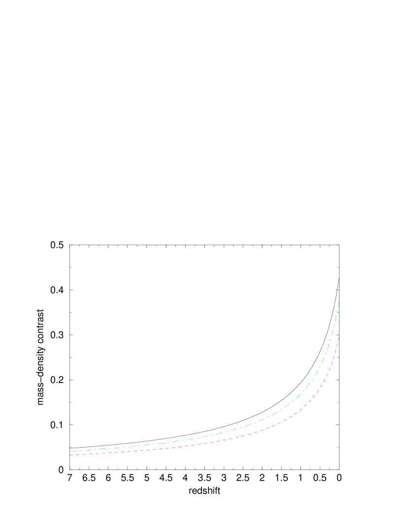
Figure 1: Mass-density contrast vs. redshift: $\delta_{i}=3.33\times 10^{-4},\ \Omega_{m}=2,\ \Sigma=0,\ 0.4\times 10^{-3},\ 0.4\times 10^{-3}a^{-1/2}$ denoted, respectively, by solid, dashed and dot-dashed lines.

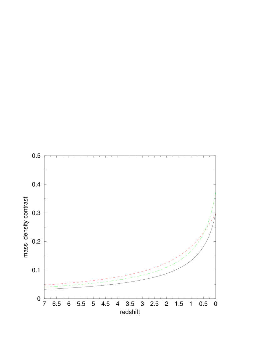
Figure 2: Mass-density contrast vs. redshift: $\delta_{i}=3.33\times 10^{-4};\ 3.33\times 10^{-4};\ 2.9\times 10^{-4},\ \Omega_{m}=2;\ 0.3;\ 2;\ \Sigma=0.4\times 10^{-3};\ 0;\ 0.8\times 10^{-3}a^{-1/2}$ denoted, respectively, by solid, dashed and dot-dashed lines.

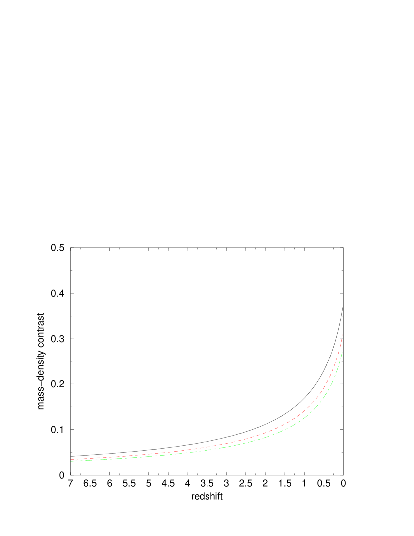
Figure 3: Mass-density contrast vs. redshift: $\delta_{i}=3.33\times 10^{-4};\ 3.33\times 10^{-4};\ 2.9\times 10^{-4},\ \Omega_{m}=2;\ 2;\ 2,\ \Sigma=0.4\times 10^{-3}a^{-1/2};\ 0.8\times 10^{-3};\ 10^{-3}$ denoted, respectively, by solid, dashed and dot-dashed lines.

3 Discussion and conclusions

From the preceding section we may conclude that the mass density contrast in the matter dominated era is substantially affected by the small amount of acceleration beyond the Robertson-Walker geometry although rendering the mass density almost unaffected. Similar conclusions one may also expect for baryon matter, but then the collisions (Peebles, 1980, Padmanabhan, 1993) should be also included in the evolution calculus.

It is evident that smaller initial density fluctuation can be compensated by larger (but still small) acceleration parameter resulting in similar behaviour of density contrast at smaller redshifts. Such an adjustment can also be made for different mass-density models.

Some cosmic observables depend on both density and density contrast, while others depend on only one of them. These can be a source of confusion if the geometry of the Universe contains acceleration. For example, the theoretical analysis of the CMBR implies equations of coupled multicomponent fluid depending on all relevant cosmic variables including density and its contrast. The small power at largest distances, as observed in the first year data of WMAP, is probably due to the integrated Sachs-Wolfe effect of the EC model with the negative cosmological constant, while the small scale structure calculations should be implemented with nonvanishing acceleration. On the other hand, the XMM X-ray cluster data analysts claim large mass density, in apparent contradiction with data sensitive to density contrasts.

To conclude, it is obvious that only a more general geometry of spacetime with the inclusion of expansion, rotation, acceleration, shear, torsion and definite EC cosmology prediction for the cosmological constant (Palle, 1996a) can save us from rather speculative considerations. In addition, the SU(3) conformal gauge theory (Palle, 1996b) supplies mass and spin of the matter content for the Universe: cold and hot dark matter as heavy and light neutrinos, respectively, baryons, charged leptons and the photon. The very fine future measurements of gravity by the LATOR mission, for example, at the solar system scale could be a complementary way to find a value of the cosmological constant.

***
I avoid referencing observational or experimental work because of extremely overwhelming number of papers with fantastic technological achievements and physical results that could produce a large number of reference-list pages. I apologize to all these astrophysicists and refer the reader to e-print archieves and web-sites of the corresponding projects.

References

- (1) Chen, X. and Kamionkowski, M. 2003, astro-ph/0310473
- (2) Kolb, E. W. and Turner, M. S., 1990, The Early Universe (Redwood City: Addison-Wesley Pub. Comp.)
- (3) Li, L.-X. 1998, Gen. Rel. Grav., 30, 497
- (4) Maskawa, T. and Nakajima, H. 1974a, Prog. Theor. Phys., 52, 1326
- (5) Maskawa, T. and Nakajima, H. 1974b, Prog. Theor. Phys., 54, 860
- (6) Padmanabhan, T. 1993, Structure formation in the Universe (Cambridge: Cambridge University Press)
- (7) Palle, D. 1996a, Nuovo Cimento B, 111, 671
- (8) Palle, D. 1996b, Nuovo Cimento A, 109, 1535
- (9) Palle, D. 1999, Nuovo Cimento B, 114, 853
- (10) Palle, D. 2000, Nuovo Cimento B, 115, 445
- (11) Palle, D. 2001a, Nuovo Cimento B, 116, 1317
- (12) Palle, D. 2001b, Hadronic J., 24, 87
- (13) Palle, D. 2001c, Hadronic J., 24, 469
- (14) Palle, D. 2002a, Nuovo Cimento B, 117, 687
- (15) Palle, D. 2002b, hep-ph/0207075
- (16) Peebles, P. J. E. 1980, Large scale structure of the Universe (Princeton: Princeton University Press)
- (17) Weinberg, S. 1972, Gravitation and cosmology (New York: J. Wiley and Sons, Inc.)