On the reliability of the black hole mass and mass to light ratio determinations with Schwarzschild models

Abstract

In this Letter, we investigate the claim of Valluri et al. (2003), namely that the use of Schwarzschild dynamical (orbit–based) models leads to an indeterminacy regarding the estimation of the free parameters like the central black hole mass and the stellar mass–to–light ratio of the galaxy under study. We examine this issue with semi–analytic two–integral models, which are not affected by the intrinsic degeneracy of three–integral systems. We however confirm the Valluri et al. result, and observe the so–called widening of the $\chi^{2}$ contours as the orbit library is expanded. We also show that, although two–dimensional data coverage help in constraining the orbital structure of the modelled galaxy, it does not in principle solve the indeterminacy issue, which mostly originates from the discretization of such an inverse problem. We show that adding regularization constraints stabilizes the confidence level contours on which the estimation of black hole mass and stellar mass–to–light ratio are based. We therefore propose to systematically use regularization as a tool to prevent the solution to depend on the orbit library. Regularization, however, introduces an unavoidable bias on the derived solutions. We hope that the present Letter will trigger some more research directed at a better understanding of the issues addressed here.

1 Introduction

A recent paper by Valluri, Merritt & Emsellem (2003; hereafter VME03) demonstrated that axisymmetric orbit–based modelling algorithms have only a limited ability to recover two fundamental parameters characterizing the total mass distribution, namely the stellar mass–to–light ratio $\Upsilon{}$ and the black hole (BH) mass $M_{\bullet}$. These authors showed that if the number of orbits is increased, the confidence contours defining the best fit values for [$M_{\bullet}$; $\Upsilon{}$] and their associated error bars widen up, hence significantly increasing the uncertainty of the BH measurement (see e.g., their Figure 3). In the case of M32, they showed that a range of models with $M_{\bullet}$ values between $1\times 10^{6}M_{\sun}$ and $6\times 10^{6}M_{\sun}$ provide equally good fit to the data discussed by van der Marel et al. (1998). This contrasts with the claim of other groups, e.g., “the range of black hole mass uncertainties is from 5% to 70%, with an average uncertainty around 20 %” (Gebhardt 2003).

We have investigated this question using component–based $f(E,L_{z})$ models, where $f(E,L_{z})$ is the distribution function (DF) depending only on the energy $E$ and the vertical angular momentum $L_{z}$ (Sect. 2). We confirm the same widening effect reported by VME03, albeit with two–integral models instead of three–integral models. In Sect. 2.3 we argue that the specific effect we describe here is due to the discretization of phase–space (i.e., the sampling into a finite number of orbits or components) and is therefore not related to the peculiar form of the distribution function.

We illustrate our claim within a realistic context, namely using the luminous mass model, as well as the SAURON and OASIS setups (Bacon et al. 2001, de Zeeuw et al. 2002) for NGC 3377 (see Copin et al. 2003, hereafter C03): these are described in Sect. 2.

We have considered two options in order to examine the reliability of the $\Upsilon{}$ and $M_{\bullet}$ determinations. First, we have investigated whether the spatial extension of the data helps to better constrain the model (Sect. 3). Second, we have included regularization in the fitting process (Sect. 4) and show that it provides a way to stabilize the widening effect in the two–integral case.

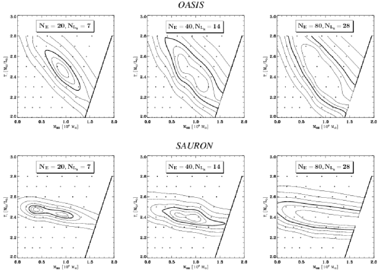
Figure 1: $\chi^{2}$–contours without any regularization. Models including only the OASIS constraints are shown on the top row, whereas the bottom row displays models with only the SAURON constraints. The number of components increases from left to right (see insets). The third, thicker, contour (counting from the innermost one) corresponds to the formal 99.7% confidence level with two degrees of freedom.

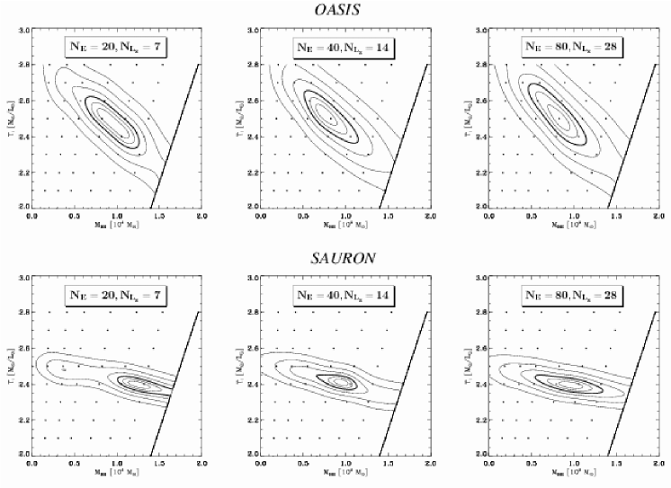
Figure 2: Same as figure 1 but for models including regularization

2 Input constraints and dynamical modelling

2.1 A two–integral model

One of the advantages of working with a two–integral DF is uniqueness: there is a unique $f(E,L_{z})$ DF that matches simultaneously the mass density, which is related to the even part of the DF, and the mean velocity field which is fully specified by the odd part of the DF (see e.g., Merritt 1996b). There is therefore no intrinsic degeneracy in recovering the input parameters [$M_{\bullet}$; $\Upsilon{}$] for the two–integral models. Note, however, that in the three–integral case the model has some additional freedom to adjust its orbital anisotropy (e.g., in the three–integral case, the radial velocity dispersion can be different than the vertical one). Thus, three–integral models with [$M_{\bullet}$; $\Upsilon{}$] values very different from the true input values may still be found to fit the data equally well (see VME03). Because of this extra freedom, the confidence level contours will always be larger in the three–integral case.

Another advantage of the two–integral models is that we can easily check directly their entire dynamical structure by comparing the reconstructed DF with the true input DF. In our view, these two properties make the two–integral case a genuine test case.

2.2 The mass model and kinematic constraints

For the luminous density distribution we use our Multi–Gaussian Expansion (MGE) model of NGC 3377 (see C03, and Emsellem et al. 1994). The stellar $\Upsilon{{}_{I}}$ has been fixed to 2.4 and a dark component in the form of a $10^{8}$ $M_{\sun}$ black hole has been included at the center: this fixes the gravitational potential of our axisymmetric model.

Except for a few notable cases (see e.g., Cappellari et al. 2002; Verolme et al. 2002, C03), the vast majority of BH determinations are based on one–dimensional long–slit spectra, leaving most of the $(x^{\prime},y^{\prime})$ sky plane unconstrained. One might reasonably expect that data densely covering the projected plane of the sky $(x^{\prime},y^{\prime})$ would help to constrain the models. This is indeed emphasized in Verolme et al. (2002) and in C03, where it is shown that the estimates of the free parameters of the models (e.g., inclination, $M_{\bullet}$, $\Upsilon{}$) are significantly better constrained when two–dimensional photometric and kinematic data are included. We have therefore tested two different regimes, namely with two–dimensional constraints having different spatial extensions (see C03; Bacon et al. 2001):

1. a central dataset, with the characteristics of the OASIS setup covering the inner $4^{\prime\prime}$ by $2^{\prime\prime}$ and,

2. a spatially extended dataset, with the full SAURON field of view covering $46^{\prime\prime}$ by $42^{\prime\prime}$.

From the MGE mass model, we have generated artificial kinematic constraints assuming a semi-isotropic distribution function $f(E,L_{z})$ using the Hunter–Qian (1993) method (HQ hereafter). The even part of such a distribution function (DF) is uniquely specified by the MGE mass model, and we chose the odd part so as to roughly mimic the observed SAURON and OASIS kinematics of NGC 3377 (C03). The observables of the HQ model (i.e., the line–of–sight velocity profiles, hereafter VPs) are then computed for both setups: they are convolved with the appropriate point spread functions and binned into the respective spatial elements, and will be used to constrain the dynamical models.

2.3 The $f(E,L_{z})$ component–based Schwarzschild models

We now turn to the building of a Schwarzschild dynamical model constrained by the fake photometric and kinematic datasets described in Sect. 2.2. We use the $f(E,L_{z})$ component–based models of Cretton et al. 1999 (hereafter C99). These authors described how to derive two–integral models (with or without central black holes) using only these $f(E,L_{z})$ components. These models were fully specified by reconstruction of the corresponding DFs (see their Figs. 6, 7 and 8), which were compared to the true underlying DFs obtained via the HQ method (see Verolme & de Zeeuw 2002 for similar computations). Following C99, and using the gravitational potential corresponding to the MGE mass model (Sect. 2), we have created a library of two–integral components by sampling the energy $E$ with ${\rm N}_{E}$ values and, at each energy, by sampling the angular momentum $L_{z}$ with ${\rm N}_{L_{z}}$values. The final solutions are obtained with a non–negative least square algorithm (NNLS, see C99 and Lawson & Hanson 1974 for details).

In the next Sections, we show that the widening effect reported by VME03 is also present with two–integral models, despite the absence of an intrinsic degeneracy for such models.

3 Spatial extension

Figure 1 shows the $\chi^{2}$ contours obtained without regularization using 1. only the OASIS constraints, covering the central parts (top row), or 2. only the SAURON constraints with a large field of view (bottom row).

The OASIS contours exhibit a clear correlation between the $M_{\bullet}$ and $\Upsilon{{}_{I}}$: a higher black hole mass needs to be compensated by a lower $\Upsilon{{}_{I}}$. With their spatial extension, the SAURON–like observables provide a much better constraint on $\Upsilon{{}_{I}}$, but obviously fail to restrict the allowed range for $M_{\bullet}$. This is an expected behaviour for such models, as discussed in details in C03. What is more surprising is that for both cases, when the number of components ${\rm N_{comp}}$ is increased, a larger region of the $[M_{\bullet};\Upsilon{{}_{I}}]$ plane is enclosed by the 99.7% confidence level ($3\sigma$ error in two degrees of freedom, which corresponds to $\Delta\chi^{2}=11.8$, see Press et al. 1992). We have increased ${\rm N_{comp}}$ by up to a factor of 16 and still, we see no sign of convergence. Using our two–integral models, we therefore see an effect similar to the one reported by VME03.

The wider field of view does not seem to stop the $\chi^{2}$–contours from getting broader; as emphasized by the bottom row of Fig. 1, it merely slows the effect down. However for the SAURON setup, we can still observe a significant increase in the allowed range of $\Upsilon{{}_{I}}$ (i.e., within the $3\sigma$ contour), particularly when ${\rm N}_{E}=80$ and ${\rm N}_{L_{z}}=28$.

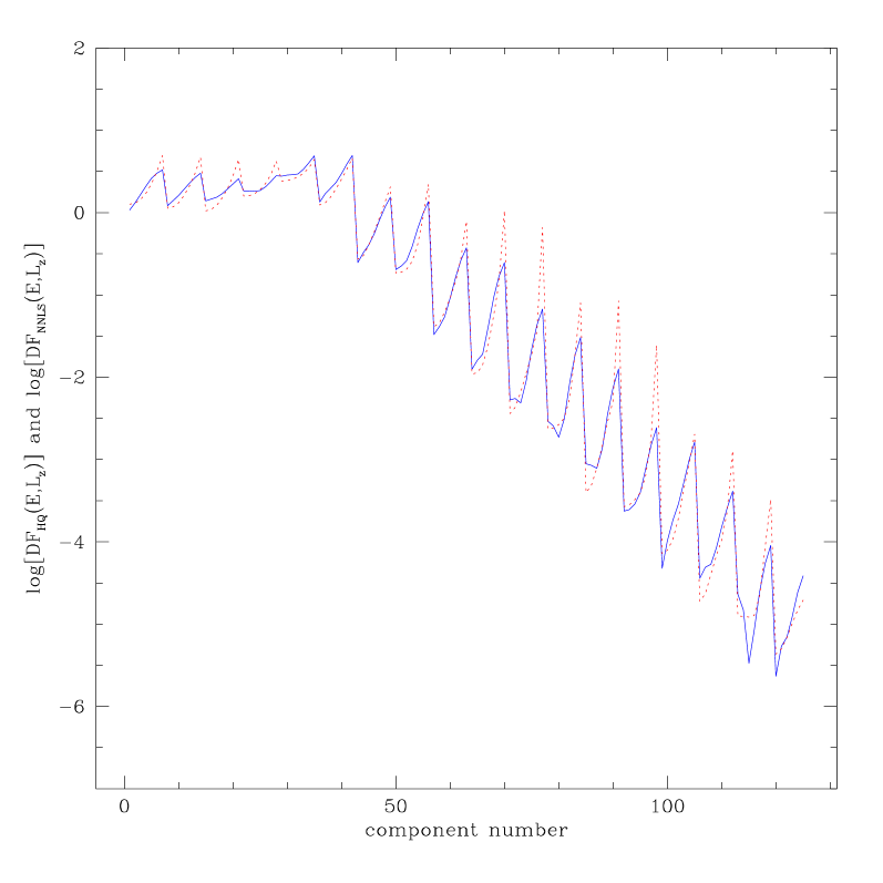
Figure 3: Distributions functions: the dotted line is the “true” ${\rm DF_{HQ}}(E,L_{z})$ derived using the HQ algorithm and the full line is the reconstructed ${\rm DF_{NNLS}}(E,L_{z})$ of the model with $[M_{\bullet};\Upsilon{{}_{I}}]$=$[10^{8};2.4]$.

4 Towards Regularization

In the absence of regularization, the weights of many two–integral components are set to zero by the NNLS algorithm: only ${\rm N}_{\rm const}$ components can have a non zero weight, where ${\rm N}_{\rm const}$ is the number of constraints (see C99). Such a behaviour has been emphasized by e.g., Cappellari et al. (2002), and Verolme & de Zeeuw (2002).

By increasing ${\rm N_{comp}}$ one improves the sampling of the integral space, which also corresponds to a better spatial sampling. In this sense, with a bigger library NNLS has more flexibility to fit the (same) data. An equally good fit to the data can then be obtained using a different model than the true input one. A larger fraction of the models in [$M_{\bullet}$; $\Upsilon{}$]–space are now acceptable, because NNLS has more freedom to select the appropriate orbits. The discretization of the phase space implies that the problem of recovering the orbital weights become ill–conditioned. We believe the same effect occurs with three–integral orbit–based models and suggest that it is partly at the root of the contour widening problem (VME03).

Including regularization forces all the components to have a non zero weight and therefore greatly reduces (or eliminates) this freedom. Furthermore, with such jagged weight distributions, the solutions without regularization are definitely far away from physical solutions. We do not claim that our way of performing regularization is optimal or represent in any sense what is taking place in real galaxies. As emphasized in Sect. 3 and in VEM03, unregularized solutions will depend on the size of the orbit library used in the analysis. However, regularization introduces an unavoidable bias in the solutions the algorithm will find.

Regularization is done here in the same way as described in C99, i.e., by minimizing the second derivatives of the weights on a grid in Integral space.

4.1 Results

Figures 2 shows the results (as $\chi^{2}$ contours) of using the OASIS (top row) or SAURON (bottom row) constraints, when regularization is included. The amount of regularization was set such as to optimally reproduce the input HQ–DF (see Fig. 8 of C99). Some other schemes to tune the optimal regularization parameter exist (e.g., generalized cross–validation, Wahba 1990; Merritt 1997).

In both SAURON and OASIS setups, the contours are stable in the sense that, while increasing ${\rm N_{comp}}$ by up to a factor 16, they do not show the widening effect observed without regularization. This can be intuitively understood by examining the size of the matrix problem which NNLS is trying to solve. Without regularization, the input matrix containing the observables for each component has ${\rm N_{comp}}$ columns (number of components) and ${\rm N}_{\rm const}$ lines (number of constraints). When ${\rm N_{comp}}$ is increased reaching values significantly larger than ${\rm N}_{\rm const}$, the problem becomes strongly underconstrained, and most of the resulting weights are set to zero (see above). When regularization is introduced, the number of columns stays constant, while the number of lines becomes ${\rm N_{comp}}+{\rm N}_{\rm const}\times{\rm N}_{\rm Int}$ ( ${\rm N}_{\rm Int}$ is the number of integral of motions, equal to 2 in the present two–integral case). As ${\rm N_{comp}}$ is increased, the numbers of columns and lines of the matrix increase simultaneously, their ratio converging to $1/{\rm N}_{\rm Int}$. Although it depends on the regularization scheme used, these additional constraints can thus qualitatively change the nature of the inverse problem.

We should emphasize here that the results presented in this Section are no proof that the contours will not get wider for a much larger ${\rm N_{comp}}$. Nevertheless, it is clearly an improvement over the unregularized case, the results of which depend on the size of the orbit library.

4.2 Distribution functions

A more conclusive test is to examine the DF corresponding to the weights recovered by the least–square routine. Figure 3 compares the reconstructed ${\rm DF_{NNLS}}$ obtained from the NNLS fit to the input ${\rm DF_{HQ}}$ derived from HQ. For each value of the Energy, $L_{z}$ runs monotonically from $L_{z,{\rm min}}$ to $L_{z,{\rm max}}$, covering ${\rm N}_{L_{z}}$ (=7 here) components. The next component corresponds to the next value of the energy, etc. Overall, the agreement is good, except for discrepancies at the peaks near $L_{z,{\rm max}}$. A similar test presented by C99 on a fake model of M 32 showed a significantly better fit (with RMS residuals of the order of a few percents). The difference lies certainly in the contribution of a disk–like component in the fake model of NGC 3377, which would probably require a better sampling in ${L_{z}}$. It is likely that some more advanced regularization scheme could improve the recovery of these steep gradients in the DF, but this is outside the scope of the present paper.

5 Comparison with other models

Gebhardt (2003) claimed that increasing the number of orbits does not produce the contour widening effect described in VME03 and in the present paper. The cause for this discrepancy is, at the moment, unclear to us.

Models with and without regularization look surprisingly si–milar when ${\rm N}_{E}$=20 and ${\rm N}_{L_{z}}$=7, which are typical values used in many orbit–based dynamical models (see e.g., vdM98, C99, Cretton & van den Bosch 1999, Verolme et al. 2002, Cappellari et al. 2002). We suggest that this coincidence has (at least) two consequences. Firstly, this could trigger the misconception that regularization does not affect the indeterminacy in the estimation of [$M_{\bullet}$; $\Upsilon{}$], since the $\chi^{2}$ contours (with or without regularization) are similar. Secondly, this could explain the good apparent agreement sometimes found between regularized and unregularized codes. If this comparison had been performed using a much larger number of orbits (in the unregularized case), we predict that a different conclusion would have been reached.

6 conclusion

In this Letter, we have used two–integral models to test the claim made by VME03 that $\chi^{2}$ contours derived using the Schwarzschild orbit-based technique widen as the orbit library is expanded.

• We confirm this effect with two–integral models for which the intrinsic degeneracy discussed in VME03 does not exist.

• We show that the widening of the $\chi^{2}$ contours occurs even when we use two–dimensional kinematics constraints.

• We suggest that the origin of such an effect partly lies in the discretization of phase space.

• We finally propose to systematically use regularization as a way to stabilize the $\chi^{2}$ diagrams produced by such techniques, so that the obtained solution does not significantly depend on the input orbit library.

Regularization schemes have been often advocated to derive stable solutions of ill–conditioned inverse problems (e.g., Golub et al. 1999, and references therein; Merritt 1996b). The main worry associated with regularization is that it biases the solution found by the fitting algorithm (see e.g., Merritt, 1996a and Dehnen, 2001 for similar questions in N–body codes). This bias may indeed not correspond to the true characteristics of the object under study. The input two–integral DF we chose for the present test is, by construction, a smooth (semi–analytical) function of the energy and angular momentum. Our analysis shows that in this case a simple regularization scheme with the right choice of smoothing parameter can be applied to recover the full (two–integral) DF reasonably well (see also C99 for a similar demonstration on a less complex DF). When modelling real galaxies, however, there is no obvious way to select the proper level of smoothing, an incorrect choice leading to either degenerate solutions (if undersmoothed; see Fig. 1) or biased solutions (if oversmoothed). The sampling of the orbit library may be further optimized such as to ensure a relatively homogeneous coverage of the presumed components of the galaxy (core, disk, bulge, etc). As mentioned in Sect. 4.2, it is likely that an adaptive regularization scheme can be designed, e.g., taking into account some a priori knowledge (or preconception) we have on a galaxy (e.g., the presence of a bright disk).

The stability of regularized solutions however comes at the cost of an unavoidable bias. The resulting best fit parameters and confidence range for [$M_{\bullet}$; $\Upsilon{}$] in a galaxy may not necessarily reflect their true values. We emphasize that, in this Letter, we only treat the indeterminacy caused by the discrete nature of the inverse problem and not the additional degeneracy associated with 3–integral models, as reported by VME03. We therefore hope that the present Letter will trigger further studies to address these issues.

Acknowledgments

We are grateful to Karl Gebhardt, Hans–Walter Rix, Michele Cappellari, Monica Valluri and David Merritt for many fruitful discussions.

References

- [Bacon et al.(2001)] Bacon, R. et al. 2001, MNRAS, 326, 23
- [Cappellari et al.(2002)] Cappellari, M., Verolme, E. K., van der Marel, R. P., Kleijn, G. A. V., Illingworth, G. D., Franx, M., Carollo, C. M., & de Zeeuw, P. T. 2002, ApJ, 578, 787
- [Copin, Cretton & Emsellem 2003] Copin, Y., Cretton, N. & Emsellem, E. 2003, A&A, in press (astro-ph/0311387, C03)
- [Cretton et al. 1999] Cretton, N., de Zeeuw, P. T., van der Marel, R. P., & Rix, H.–W. 1999, ApJS, 124, 383
- [Cretton & van den Bosch 1999] Cretton, N. & van den Bosch, F. C. 1999, ApJ, 514, 704
- [Dehnen 2001] Dehnen, W., 2001, MNRAS, 324, 273
- [de Zeeuw et al.(2002)] de Zeeuw, P. T. et al. 2002, MNRAS, 329, 513
- [Emsellem, Monnet & Bacon 1994] Emsellem, E., Monnet, G., & Bacon, R. 1994, A&A, 285, 723
- [Gebhardt et al.(2003)] Gebhardt, K. et al. 2003, ApJ, 583, 92
-