Triangulating Radiation:
Radiative Transfer on Unstructured Grids

Abstract

We present a new numerical approach that is able to solve the multi-dimensional radiative transfer equations in all opacity regimes on a Lagrangian, unstructured network of characteristics based on a stochastic point process. Our method reverses the limiting procedure used to derive the transfer equations, by going back to the original Markov process. Thus, we reduce this highly complex system of coupled differential equations to a simple one-dimensional random walk on a graph, which is shown to be computationally very efficient. Specifically, we use a Delaunay graph, which makes it possible to combine our scheme with a new smoothed particle hydrodynamics (SPH) variant proposed by Pelupessy et al. (2003). We show that the results of applying a two-dimensional implementation of our method with various suitable test cases agree with the analytical results, and we point out the advantages of using our method with inhomogeneous point distributions, showing examples in the progress. Hereafter, we present a supplement to our method, which can be useful in cases where the medium is optically very thin, and we conclude by stating some anticipated properties of this method in three dimensions, and announce future extensions.

1 Introduction

The formation of cosmic structures, such as galaxies and stars, is almost certainly dominated by an intricate interplay between (magneto)hydrodynamics, gravity, and radiative transfer, on a cosmological background that sets the initial and boundary conditions. Of these, the cosmology is assumed to be given, while the computation of gravitational potentials is rather well understood (e.g. Greengard, 1988). Hydrodynamics must be three-dimensional for this purpose, and 3D hydro is beginning to enter its springtime: adaptive-mesh refinement (AMR) and related methods are beginning to produce results (see e.g. LeVeque, 1998, for a review). However, radiative transfer techniques that combine true three-dimensionality with reasonable spectral resolution are, by comparison, the most primitive of the methods needed for realistic simulation of structure formation. Yet it seems essential that the physics of radiation be built in, because the energy budget of nascent structures is heavily influenced, indeed sometimes dominated, by radiative effects. Serious models must be three-dimensional, and spectral coverage must at least be good enough to cover hydrogen ionisation, recombination and photodissociation. This makes solving the radiation part of the physical problem seven-dimensional: a daunting computational task.

Usually, a galaxy is represented by a finite point set, with a size of the order of $10^{6}$, in which each point represents a fixed mass fraction of the galaxy. Because these points represent thousands of solar masses or more, they are not actually point-like. Thus, one is immediately confronted with the problem that the laws of motion are differential equations that represent a continuum, which cannot be uniquely defined on a discrete point set. In order to circumvent this problem, one can convolve the set with a smoothing function so that a continuous field is obtained. In this way, gradients and other derivatives are properly defined. The scheme which combines this smoothing trick with the implementation of the equations which govern the dynamical behaviour of fluids, is called Smoothed Particle Hydrodynamics (SPH; Lucy, 1977). It has been well established that the use of SPH, under certain restrictions, can be very fruitful for doing astrophysical hydrodynamical calculations (for a review, see Monaghan, 1992).

Next, the interaction between radiation and matter must be included. The radiative transfer equations, which describe this interaction macroscopically, are a system of non-local, coupled differential equations and are extremely difficult to solve analytically and numerically (e.g. Rutten, 1999). Recently, Pelupessy et al. (2003) stated that it would be advantageous in several ways to avoid the use of a smoothing function when using SPH, and instead use the Delaunay tessellation of the point set to create a continuous field. This method is called the Delaunay Tessellation Field Estimator (DTFE; Schaap & Van de Weygaert, 2000). Accordingly, if we could find a scheme that is able to solve the radiative transfer equations on a Delaunay grid, we could combine the two, and thereby introduce radiative transfer in a natural and possibly economical way into particle-based methods such as SPH.

The aim of this paper is, to present a new numerical method that is able to solve the radiative transfer equations by means of a Markov process on networks of characteristics, such as a Delaunay graph. We adopt the Lagrangian treatment of the SPH-scheme and let the point process represent the underlying mass distribution, by which the method will be able to solve the equations in all opacity regimes. The method is extremely fast, conceptually very simple, and because of its generic setup it is applicable in spaces of any dimension.

First, we discuss the extant numerical schemes for solving the transfer equations (in three dimensions), emphasising their advantages and disadvantages, and why these are not sufficient for the needs at hand. Second, we present our new method, after which we show the results of using our method with several two-dimensional test cases. Thereafter, we point out the advantages of our method by using it on a correlated, inhomogeneous point distribution. We finish by presenting a version of our method that can be used when the medium is optically very thin.

2 Numerical radiative transfer

For our present purposes, it suffices to summarise the quantum nature of the interaction between radiation and matter by macroscopic parameters, for example a scattering cross section or a mean absorption coefficient. If we assume that the radiation relaxation time is small compared to the the other time scales of the considered physical system, we may use the time-independent (equilibrium state) Boltzmann equation for photons (in general $d$ dimensional space),

$$\mn@boldsymbol{n}\cdot\nabla I_{\nu}(\mn@boldsymbol{x},\mn@boldsymbol{n})=j_{\nu}(\mn@boldsymbol{x},\mn@boldsymbol{n})-\alpha_{\nu}(\mn@boldsymbol{x},\mn@boldsymbol{n})I_{\nu}(\mn@boldsymbol{x},\mn@boldsymbol{n}).$$ (1)

This equation relates the spatial gradient of the luminous intensity $I_{\nu}(\mn@boldsymbol{x},\mn@boldsymbol{n})$ of photons with frequency $\nu\in\mathbb{R}^{+}$ travelling in the direction $\mn@boldsymbol{n}\in S^{d-1}$, at the location $\mn@boldsymbol{x}\in\mathbb{R}^{d}$, to certain source terms. The right hand side of this equation lists the source terms for emissivity $j_{\nu}(\mn@boldsymbol{x},\mn@boldsymbol{n})$ and for extinction $\alpha_{\nu}(\mn@boldsymbol{x},\mn@boldsymbol{n})$, which includes the scattering coefficient $\alpha^{\mathrm{scat}}_{\nu}(\mn@boldsymbol{x},\mn@boldsymbol{n})$ and the pure absorption coefficient $\alpha^{\mathrm{abs}}_{\nu}(\mn@boldsymbol{x},\mn@boldsymbol{n})$.

Eq.(1) is the time-independent radiative transfer equation, which describes the radiative properties of systems in radiative equilibrium, and it is this equation that our new method solves, as we will show in what follows.

2.1 Limiting behaviour

A general analytical solution of this non-separable integro-differential equation of first order does not exist, because of its behaviour in different limiting (opacity) regimes. For example, if we take a dominating scattering cross section, that is $\alpha^{\mathrm{scat}}_{\nu}(\mn@boldsymbol{x},\mn@boldsymbol{n})D\gg 1$, with $D$ as the thickness of a layer of medium, a particular photon will be scattered many times, so that the angular dependence of the original incident angle is wiped out. It can be shown algebraically (e.g. Duderstadt & Martin, 1979) that in this limit the transfer equation Eq.(1) can be rewritten as a diffusion equation, the solutions of which are angle independent.

On the other hand we have the limit in which the scattering cross section is very small, that is $\alpha^{\mathrm{scat}}_{\nu}(\mn@boldsymbol{x},\mn@boldsymbol{n})D\ll 1$. In this case, if also $\alpha^{\mathrm{abs}}_{\nu}(\mn@boldsymbol{x},\mn@boldsymbol{n})D\ll 1$, the mean free path of a photon is very large, so that neighbouring paths need not be correlated, and there may be a different solution for each angle. In this case, the transfer equation can be rewritten as an upwind hyperbolic PDE, the solutions of which are angle dependent.

Thus, the characteristic properties of the solution in different limits can be quite contradictory, which shows the great difficulty in finding an explicit general solution to the transfer equation.

2.2 Numerical schemes

There are numerous numerical schemes that are excellent at solving the transfer equation in one of the opacity regimes. But in passing from one regime into the other most schemes fall short. A solver for the diffusion limit cannot solve the hyperbolic PDE, and vice versa. Fortunately, some schemes have been developed which, in principle, are able to solve the transfer equation in all opacity regimes. Most of these can be subdivided into three main categories: those using long characteristics, short characteristics, and the Monte Carlo methods. Because we want to point out how these relate to our new method, and in particular how ours improves on the extant ones, we briefly sketch their approach.

First, all of these methods work by superimposing a grid on the domain on which the transfer equation has to be solved. The aim is to find the intensity $I_{\nu}$ in a number of directions for each of the grid cells. In the Monte Carlo approach, one sends out $N$ photon packets from each grid cell in a certain number of random directions, and one just keeps detailed track of its scattering, absorption and re-emission. These methods are very easy to implement, it allows for very complicated spatial distribution and arbitrary scattering functions. However, because they use statistical averaging, they introduce statistical noise, which can only be suppressed by taking a large value for $N$. Because the noise reduction scales with the square root of $N$ only, Monte Carlo methods are computationally very expensive.

The long characteristics method (first suggested by Mihalas et al., 1978) uses rays (characteristics) which connect a given grid cell to every other relevant cell. The transfer equation is solved one-dimensionally along these lines. This type of method has the advantage that it incorporates the nonlocality of the transfer equation, and is thus able to solve it accurately for arbitrary density configurations. A disadvantage is that the method becomes computationally very expensive, if one wants high angular resolution, so as to accurately sample space at large distances from the source. Moreover, the long characteristics usually cover the same part of the domain many times. This introduces strong redundancy, which makes the method time-consuming.

A way around this redundancy problem is the short characteristics method (first proposed by Kunasz & Auer, 1988). In this case, one calculates the intensity in one grid cell by connecting it with its neighbouring cells only, and solves the transfer equation one-dimensionally along these lines. An advantage of this method is, that it is not very redundant, but it also requires a very clever scheme to sweep the grid, in order to be sure that the intensities in all the neighbouring grid cells are known when they are needed. This is necessary because the emissivities may depend on the intensities, for example in the case of scattering. The physical values of the neighbouring cells contribute via interpolations along the grid lines, which have to be quadratic or higher order in order to accurately reproduce the diffusion limit, which is governed by the second order diffusion equation. The interpolation, intrinsic to the short characteristic methods, introduces angular diffusion into the numerical solution, for example causing parallel laser beams to diverge in the downwind direction (e.g. see Steinacker et al., 2002). Kunasz & Auer (1988) showed that a parabolic interpolation reduces this intrinsic numerical diffusion, thereby obtaining a more accurate result, but not only does it make the algorithm more complex, because it requires three upwind interpolation points, but it can also cause unphysical under- and overshoots of the interpolated quantities near discontinuities, possibly resulting in values for $I_{\nu}$ which are negative.

To illustrate the difficulties of these methods, we present a schematic example of several radiating optically thick clouds which are surrounded by vacuum (see Fig.1).

Figure 1: Schematic illustration of several radiating clouds surrounded by vacuum.

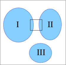
Albeit that this example is oversimplified, it is illustrative, because one immediately sees that, if we want to calculate the radiation profile of the emission of cloud II, we have to take into consideration the radiation emitted by the neighbouring clouds, because this can contribute to the desired profile via scattering and/or re-emission. Radiation emitted by cloud I will encounter sharp gradients in the opacity, when it leaves the optically thick cloud and streams freely into the vacuum, until it gets absorbed or scattered by the optically thick cloud II.

Zooming in on the square in Fig.1 we obtain Fig.2.

Figure 2: Zoom in of the square in Fig.1. Illustration of two mechanisms for calculating the effect of radiation passing through optically very thin medium, after being emitted at a point A near the border of cloud I, on the medium in the neighbourhood of a point B near the border of cloud II. Left is a schematic illustration of a long characteristic method; right is one of a short characteristic method.

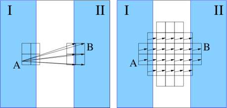
If one wants to calculate the effect of the radiation emitted at a point A near the border of cloud I on the local re-emission properties of a point B near the border of cloud II, one can take the long (Fig.2, left) and the short characteristics (Fig.2, right) approach. From the analytical solution we know that the radiation emitted by cloud I should propagate outwards as a plane wave (assuming we zoom in sufficiently for the boundary to be a straight line), with characteristics perpendicular to the outer boundary of the cloud. One thing we immediately see is that, in order to accurately simulate the plane wave, at least the whole boundary region has to be incorporated as a source, for example by sampling that region by a considerable amount of point sources. Because the operation count of both methods scales with the number of sources, an extended source like in this example will increase the required number of operations enormously, sometimes even beyond the reach of modern computer power. Moreover, most radiative transfer methods are designed to solve physical problems in which there is an inherent geometrical symmetry, most frequently axi-symmetry, or even more simple, to solve for just one point source. Of course, both these simplifications result in severe restrictions on the type of physical configuration one would like to model. Another complication, when using a long characteristic method (Fig.2, left), is that the angular sampling has to be very accurate so as to have a good sampling of space at large distances. If the distance from cloud I to cloud II increases, the accuracy and thus the number of cycle counts needed increases proportionally. In the short characteristic methods (Fig.2, right), we see that the upwind interpolation scheme gives rise to numerical, unphysical diffusion in the empty region between cloud I and II, by which the angular resolution at large distances from the source tends to get smeared, so that detailed information is lost. This effect would be even more dramatic in the case that the boundary region is inhomogeneous, which would give cause to a wave front with a rich variety of multipole features.

In addition, there is a generic drawback inherent in all these classes, which we immediately see from Fig.2: they use a stiff grid which has nothing to do with the underlying physical problem. When using those unphysical grids, one introduces preferential directions and superimposed scale lengths which are not related to the problem at hand. Because we need a grid fine enough to accurately resolve the dense structure near the boundary, we enormously oversample the optically thin region between the clouds.

The new method, which we present in the next section, is a supplement to the extant methods, in the sense that it is not restricted to just one opacity regime and that it uses a physical grid, thereby avoiding the difficulties of using an unphysical one, as we have just described. Moreover, it does not scale with the number of sources, performing equally fast for extended sources as for one point source. It is, in a sense, a combination of all three categories of radiative transfer methods, but we will elaborate on this comparison later on.

3 A new method

In his landmark paper, Chandrasekhar (1943) showed that the migration of photons through a medium can be described as a Markov stochastic process. More specifically, the migration can be described as a random walk of photons through a medium during which they may get scattered or absorbed according to the scattering coefficient $\alpha^{\mathrm{scat}}$ and the absorption coefficient $\alpha^{\mathrm{abs}}$ of the medium. A normalised phase function, $f(\mn@boldsymbol{n},\mn@boldsymbol{n}^{\prime})$, describes the probability of a photon scattering from direction $\mn@boldsymbol{n}$ to $\mn@boldsymbol{n}^{\prime}$. The free path between two consecutive events, which can either be scattering or absorption, has an exponential distribution in the form of $\alpha^{\mathrm{tot}}\mathrm{e}^{{-\alpha^{tot}D}}$, which is characterised by the total attenuation $\alpha^{\mathrm{tot}}=\alpha^{\mathrm{scat}}+\alpha^{\mathrm{abs}}$. At one such event, absorption takes place with a probability $\alpha^{\mathrm{abs}}/\alpha^{\mathrm{tot}}$ and scattering with probability $\alpha^{\mathrm{scat}}/\alpha^{\mathrm{tot}}$. This picture forms the basis for the Monte Carlo simulation of photon migration. Chandrasekhar (1943) showed that by taking a large number of steps or, equivalently, by averaging over a large number of possible paths, one can use these microscopic statistics to derive macroscopic quantities, such as the number of photons at a certain distance from the source, travelling in a certain direction, which is of course the pivotal specific intensity.

Our new method is characterised by the approach that we sample the medium by a finite amount of discrete event centres, in such a way that the volume average over a certain region containing these event centres results in the correct macroscopic physical quantities, such as the scattering and absorption optical depths, for the medium we try to model. One crucial assumption is that the ensemble of scattering or absorbing particles, i.e. event centres, is ergodic, so that the sample we choose is representative for the whole ensemble. The essential aspect of our new method is that we use this set of event centres as our set of grid points, coupled with a specific choice for their interconnection, the Delaunay/Voronoi tessellation.

3.1 The grid

We do not use a grid in the usual sense, nor do we solve a differential equation. Instead, we return to the physical origin of the equations of radiative transfer by introducing a point process on which we let photons travel by a Markov process. Thus, we use a physical grid for radiative transfer. The placement of the grid points (the point process) is determined by the underlying mass distribution, which may adapt to the dynamical properties of the medium. Thus, given a certain amount of available grid points, we put most at places where the density is highest and least in low-density areas. The exact recipe we use for placing the available points is discussed in Subsection 3.2.2.

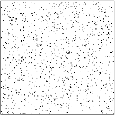
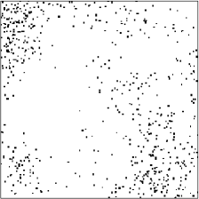
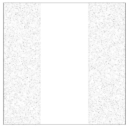
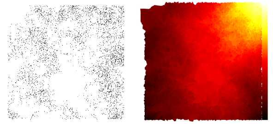
A key issue of our method is that we use a stochastic point process as a recipe for placing the points. If the underlying mass distribution were homogeneous and isotropic, we should use a Poisson process. The average amount of points within a certain area would be a constant $\rho_{\mathrm{D}}$, called the point intensity. If the medium distribution were inhomogeneous, we would have to use a correlated point process, as a result of which the point distribution would show clumpiness. Either way, we make use of a random number generator to get the coordinates of a point. This automatically simulates a Poisson point process (see Fig.3, left). In the case of a correlated point distribution, we reject some coordinates and move on to the next in such a way that the overall distribution has a density profile conforming to the underlying medium distribution (see Fig.3, right). Of course, if we have the exact $d$ dimensional density distribution function (or a discretised $d$ dimensional density array), it is always possible to use Monte Carlo methods to sample that density distribution with a finite amount of points with an accuracy that is only limited by the number of points.

Figure 3: Left: Poisson point process representing a homogeneous medium; Right: Correlated point process representing a clumpy medium.

Next, we must specify a way of connecting the grid points with a network of lines along which the photons will travel (characteristics). The nice thing about our method is that it is not very strict in what the requirements for such a connection scheme should be. This freedom in constructing a network makes it possible to use our method on many different types of grid. That said, it is of course very desirable to choose an approach that does not suffer from the drawbacks we have just criticised, such as the incorporation of a preferred length scale or preferential directions.

We choose the least restrictive unique connection method known to us: the Delaunay triangulation, although one should keep in mind that this is just one of the many possibilities. There are only two limitations to the approach presented here: 1) only ‘neighbouring’ points should be able to communicate; 2) the resultant network, or grid, should be a simple and connected graph, i.e. two points are connected by at most one line segment and there is a path from any point to any other point in the graph. In this way, we create what is called an unstructured grid, to distinguish it from grids with systematic properties such as cell size or wall direction.

3.1.1 Voronoi/Delaunay tessellation

The Delaunay triangulation (Delaunay, 1934) and its mathematical dual, the Voronoi tessellation (Voronoi, 1908), is one of the mainstays of stochastic geometry. We will briefly discuss its properties. For more details, we refer to Stoyan et al. (1996) and Okabe et al. (2000).

A tessellation is an arrangement of polytopes which fit together without any overlap, completely covering a certain domain. Usually these cells are convex, which means that every line connecting any two points within the cell is also within the cell. A very important and exhaustively studied category of tessellations is the Voronoi tessellation. It is widely applicable in numerous branches of theoretical and applied science, from astrophysics to zoology (e.g. Van de Weygaert, 1991).

Given a stationary point process $\Phi$, of nuclei $\{x_{i}\}$ in $\mathbb{R}^{d}$, which has a finite intensity $n$, the Voronoi tessellation is defined as

$$V(\Phi)=\{C_{i}\},$$ (2)

in which

$$C_{i}=\left\{y\in\mathbb{R}^{d}:\left\|x_{i}-y\right\|\leq\left\|x_{j}-y\right\|\forall x_{i}\neq x_{j}\right\}.$$ (3)

That is to say, the Voronoi cell $C_{i}$ is the set of all points closer to $\mn@boldsymbol{x}_{i}$ than to all other points.

If two Voronoi cells $C_{i}$ and $C_{j}$ have a common $(d-1)$-facet (in two dimensions an edge, in three dimensions a wall, etc.), they are said to be contiguous to each other. By joining all the nuclei whose cells are contiguous, we obtain a set of simplices (a simplex is the generalisation of a tetrahedron in $d$-dimensional space). Thus, we obtain a second form of tessellation based upon the same point process. This is the Delaunay triangulation, and its simplices are called Delaunay triangles, tetrahedra, etc.

3.2 Transfer along the Delaunay network

3.2.1 Continuous or discrete transfer

Once a grid has been defined, we must specify a method by which the radiation is supposed to travel along the grid lines. The usual way is, to compute the entire propagation along each path segment, i.e. to integrate the one-dimensional version of the equation of radiative transfer. This necessarily entails two problems: first, the necessity of designing a subgrid model (i.e. an approximation of the optical properties within a computational cell); second, the computer-intensive effort of calculating this integral for each grid line.

Our approach is different: instead of applying continuous transfer, we move the radiation without further processing from node to node. Remember that we do not use an underlying grid which is then crossed by the photon characteristics; we dispense with the grid altogether and use a point-to-point propagation of the radiation. By taking this approach, each Delaunay line is equivalent to each other one. Of course, this means that the point distribution only represents the density, and cannot be directly proportional to the density, except in the homogeneous case; otherwise, the intensity of a point source would not decrease exponentially in an absorbing atmosphere. We are therefore obliged to find a suitable mapping between the density distribution of the medium and the discrete points representing it. We use a local criterion which uniquely determines this mapping: we require the optical mean free path to be locally the same for the exact exponential solution and the point-to-point transfer.

Let a particular photon line start at coordinate $0$, and end at a distance $x$. Assume that our point sampling is so fine that the density is approximately constant between these points; in other words, $\frac{1}{\rho}\frac{\partial\rho}{\partial x}<\frac{1}{\lambda_{\mathrm{D}}}$, where $\lambda_{\mathrm{D}}$ is the mean length of a local Delaunay line. Then the radiation arrives at $x$ with an attenuation $e^{-x/\lambda}$, where $\lambda$ is the photon mean free path. Now we sample the segment $(0,x)$ with $N$ points, at each of which a fraction $c$ of the radiation is taken away. Thus, the discrete propagation attenuation becomes

$$(1-c)^{N},$$ (4)

in which $c$ is a global constant (to be considered below) and in which $N=x/\lambda_{\mathrm{D}}$. To first order, this expression is equal to the exponential attenuation, if

$$x/\lambda=Nc=cx/\lambda_{\mathrm{D}},$$ (5)

so that

$$\lambda_{\mathrm{D}}=c\lambda.$$ (6)

The question is which recipe to use for distributing the grid points in such a way that the optical mean free path $\lambda$ locally is represented correctly via Eq.(6).

3.2.2 Placing the points

We base our point distribution on the local properties of the medium. From basic radiative transfer theory, we know that $\alpha^{\mathrm{abs}}=\rho\kappa^{\mathrm{abs}}$ and $\alpha^{\mathrm{scat}}=\rho\kappa^{\mathrm{scat}}$, where $\kappa^{\mathrm{abs}}$ and $\kappa^{\mathrm{scat}}$ are the mass absorption coefficient and the mass scattering coefficient, respectively. Because the mean free path $\lambda=1/\alpha$, we know that locally

$$\lambda(\mn@boldsymbol{x})=1/\kappa\rho(\mn@boldsymbol{x}).$$ (7)

Given a local grid point density $\rho_{\mathrm{D}}(\mn@boldsymbol{x})$, we know from stochastic geometry that the average Delaunay line length $\lambda_{\mathrm{D}}(\mn@boldsymbol{x})$ in that region locally will have length

$$\lambda_{\mathrm{D}}(\mn@boldsymbol{x})=\zeta/\rho_{\mathrm{D}}(\mn@boldsymbol{x})^{1/d},$$ (8)

in which $\zeta$ is some constant geometrical factor, which depends on the dimension $d$ and has been evaluated in, for example, Okabe et al. (2000), as

$$\zeta_{2D} = \frac{32}{9\pi}\approx 1.132$$ (9)

$$\zeta_{3D} = \frac{1715}{2304}\left(\frac{3}{4\pi}\right)^{1/3}\Gamma\left(\frac{1}{3}\right)\approx 1.237.$$ (10)

We can conclude from Eqs.(7) and (8) that, if we choose our point distribution to sample the $d$-th power of the density, i.e.

$$\rho_{\mathrm{D}}(\mn@boldsymbol{x})=\frac{\rho^{d}(\mn@boldsymbol{x})}{\int_{D}\rho^{d}(\mn@boldsymbol{x})}N,$$ (11)

in which $N$ is the total amount of grid points available and $D$ the volume of our computational domain, the length of a Delaunay line $\lambda_{\mathrm{D}}(\mn@boldsymbol{x})$ between two event centres, or grid points, will scale linearly with the local mean free path of the medium $\lambda(\mn@boldsymbol{x})$ via a constant $c$. That is

$$\lambda_{\mathrm{D}}(\mn@boldsymbol{x})=c\lambda(\mn@boldsymbol{x}).$$ (12)

Thus, because we choose the point distribution to conform to the density profile of the medium according to Eq.(11), the average Delaunay line length and the mean free path have the same $\rho^{-1}$ dependence, by which Eq.(12) is a global relation with a global constant $c$. We will explicitly derive the important constant $c$ later on. In other words, by adopting the sampling criterion in Eq.(11) we have accounted for the difference between integrating the propagation along a Delaunay line, and using a discrete point-to-point propagation.

Unless we have an enormously high amount of points available, the average local geometrical mean free path of our graph, $\lambda_{\mathrm{D}}$, will be a lot bigger than the local physical microscopic scattering mean free path $\lambda^{\mathrm{scatt}}$. In other words, we expect that $c^{\mathrm{scatt}}\gg 1$. Thus, we will define each of the grid points to be a scattering centre, where possibly another event can occur, e.g. (partial) absorption. Of course, $\lambda^{\mathrm{abs}}$ need not be equal to $\lambda^{\mathrm{scatt}}$, but we take care of this by choosing a suitable numerical transfer recipe.

The only problem occurs, when $\lambda^{\mathrm{scatt}}$ becomes bigger than the size of our computational domain. In this case, the domain should not contain any event centres, and should thus be devoid of grid points. We shall tackle this problem towards the end of this paper. For now, we shall assume that $\lambda^{\mathrm{scatt}}$ is smaller than the dimension of our computational domain.

3.2.3 Propagation

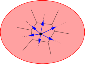
Now let us proceed to radiative transfer on this grid, or graph. From now on we will use two-dimensional examples to illustrate the mechanism, but in every case the generalisation to $d$-dimensional space is either trivial, or else explicitly clarified. Let us consider the example in which there is a blob of matter which acts as a source of radiation. According to what was said before, we have to put a number of grid points within the blob, according to the $d$-th power of its density distribution. We know that each point is surrounded by a Voronoi cell, and we assume that the Voronoi cells are small enough (i.e. the number of points $N$ is high enough) to accurately fill the blob, according to some criterion $\frac{1}{\rho}\frac{\partial\rho}{\partial x}<\frac{1}{\lambda_{\mathrm{D}}}$. Now we use each of these points as a source, which means that we send an equal amount of source photons out of this point along each of the Delaunay lines which emerge from it. An illustration of this example can be seen in Fig.4, in which we exaggerated the size of one Voronoi cell. We show a Voronoi cell with its neighbours and the dashed lines indicate the Delaunay lines.

Figure 4: A blob of radiation (red shaded) is subdivided in a high number of Voronoi cells, each of which surrounds one grid point. We magnify one of these Voronoi cells and show how the source radiation is sent along the dashed Delaunay lines into the neighbouring Voronoi cells.

Figure 5: Left: The radiation in the shaded area is projected onto the Delaunay edge and propagates along it. Right: When it comes upon an intersection, it is split up according to a certain recipe which depends on the events taking place at this event centre.

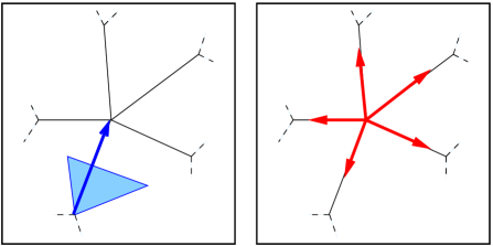
Thus, the whole domain is subdivided unambiguously by the Voronoi cells and the radiation is projected onto the Delaunay network. The only thing left to be specified is a way to let the source radiation propagate solely along the resultant Delaunay line network, from one event centre to the next. Zooming in on one grid point (see Fig.5, left), which is connected to a number of others, we see that the source radiation within the shaded area, which is a certain part of the original Voronoi cell, is projected onto the Delaunay edge. It propagates along that edge until it reaches the next point, where a number of Delaunay lines meet. Because this grid point is a scattering centre, the radiation will be sent away out of the cell along all the Delaunay line (see Fig.5, right), and propagates onwards along the graph until it reaches the next event centre where we can use the same general recipe, because of the Markovian properties of this random walk. Moreover, we are at liberty to put in all kinds of radiation-matter interactions (e.g. absorption, re-emission, multi-frequency redistribution, ionisation, recombination) between the arrival and scattering of the radiation packet, but we will elaborate on this later.

Thus, we have split the radiative transfer equation into two parts: 1) we let the radiation interact with the medium at each event centre, after which 2) we advect the radiation along the Delaunay lines towards the next event centre. By making this choice, we have reduced the radiative transfer to its microscopic origin: a random walk of photons between scattering centres. As said, the physical mean free path of photons is not the same as the mean length of our Delaunay lines, so this Markov process does not coincide with the microscopic physical case. Even so, we believe that it retains the essentials (cf. Eq.(12)), while removing the grid-dependent systematic effects mentioned above in the previous section.

3.3 A physical grid

To illustrate the optimal physical properties of the geometry of the grid, we mention again that by choosing the point distribution properly the average length of a Delaunay line, and thus the average width of a Voronoi cell, scales linearly with the local mean free path of the photon (cf. Eq.(12)), by which the scale length is not some superimposed unphysical measure, but directly related to the physical properties of the medium. Moreover, because we use a stochastic point process to place the grid points, the angle between two lines meeting at one of these points will also have a stochastic nature, which removes the unphysical fixed preferential directions superimposed by the numerical methods mentioned in Section 2. In order to show an example of the type of grid we obtain by using our method, we return to the example used in Fig.2. Using our recipe for placing grid points according to the medium density profile, we obtain the result depicted in Fig.6, top.

Figure 6: Top: Point distribution for a medium distribution as in Fig.2. Bottom: Resultant Delaunay network of characteristics along which the radiation can propagate.

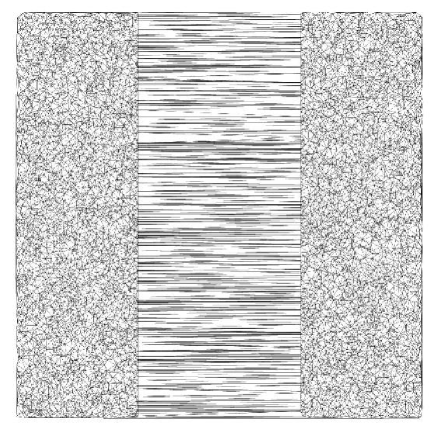
In the bottom part of Fig.6, one can see the result of making a Delaunay tessellation of this point distribution. One can readily see that the length of the Delaunay lines, that is the characteristics along which the radiation can propagate, correlates with the mean free path. The Delaunay lines emerging from the grid points at the boundary of cloud I are very long and causally connect cloud I with cloud II. The Delaunay lines are precisely the emergent perpendicular characteristics of the plane wave moving through the optically thin region. Because nothing happens to the radiation packet as it moves in a straight line along these characteristics to the first event centres in cloud II, the numerical diffusion is minimal compared to what we would get using a short characteristic method.

Another advantageous property of a Delaunay network is that it increases the angular resolution in cases where it is needed. If we would have a homogeneous medium distribution full of scattering centres that are distributed according to a Poisson point process, the resultant Delaunay graph has some properties that can be evaluated analytically (for a summary, see Okabe et al., 2000). One of these is the average number of $d-1$ facets of a $d$ dimensional Poisson-Voronoi cell, that is the number of sides in two or the number of walls in three dimensions. These are $6$ and $(48\pi^{2}/35)+2\approx 15.54$, respectively. The normal of each $d-1$ facet is a Delaunay line, thus the number of $d-1$ facets of each Voronoi cell corresponds to the number of Delaunay lines joining at an event centre or, equivalently, the amount of (solid) angles into which the radiation can be scattered (see Fig.5). Because the possible directions for the homogeneous medium is on average $6$ (in 2D), the angular resolution is not very good. But this poses no problem, because, as we argued in Section 2, in this case of a high scattering opacity the angular dependence tends to get wiped out. The angular resolution is of importance, when radiation is sent out into an optically thin region. Therefore, the angles between the Delaunay lines connecting a grid point near the boundary of cloud I to one in cloud II have to be small. We will more rigorously show in a later section of this paper that a Delaunay tessellation based on a stochastic inhomogeneous point process has the property that the angle between long Delaunay lines will be much smaller than the angle between short Delaunay lines.

Another elegant property of our grid is that it is reciprocal, or time-reversible. In a short-characteristics scheme, we need to devise a clever downwind sweeping and interpolation scheme to know the influence of an upwind source A on a downwind point B (cf. Fig.2). If we want to turn things around, and try to calculate the influence of point B on point A, the overall cascade of computations will, in general, differ. In a long characteristic method, we would create a high number of isotropically distributed rays at point A, one of which hopefully passes nearby point B, but one would need to create a whole new set of rays around B to calculate its effect on cloud I. Our grid has an inherent symmetry, in that we know that the trajectory of a photon packet sent out from point A across the network to point B will be the same for a photon sent out from point B to point A. This is the best example of what we already mentioned earlier, that our grid is not designed for one specific geometrical symmetry, as so many of the extant numerical methods, but that it is symmetrically optimised for each grid point.

3.4 Event centres

As we have pointed out earlier, our new method splits the radiative transfer equation into two parts: one advection part, and one interaction part. It’s at the event centres, or grid points, where the radiation-matter interaction takes place. In the previous, we defined each event centre to be at least a scattering centre, where the radiation is redistributed according to the recipe in Fig.5, right. But our method gives us the liberty to incorporate a wide variety of radiation-matter interactions in between the arrival and scattering of the radiation, such as absorption, ionisation, re-emission, recombination, etc.

3.4.1 Absorption

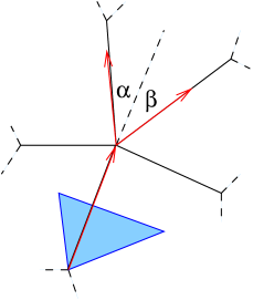
Suppose one wants to simulate the propagation of photons through an absorbing medium, or, more specifically, one wants to determine the radiation intensity profile as a result of a certain distribution of sources in a medium with a mass absorption coefficient $\kappa^{\mathrm{abs}}$. If this medium is inhomogeneous, the density can change dramatically from one point to the next, so that the value of the absorption coefficient (via $\alpha^{\mathrm{abs}}=\rho\kappa^{\mathrm{abs}}$) can have widely varying values at different places. Because we have designed our method in such a way that our point distribution follows the medium distribution according to Eq.(11), we can assign a global constant to each grid point.

What is the value of this constant? Let us examine Fig.7, in which a typical Voronoi cell which surrounds an event centre is depicted. Radiation comes in from a neighbouring Voronoi cell along a Delaunay line (blue arrow), and, before it is scattered, some part of it is absorbed according to the local optical depth $\Delta\tau^{\mathrm{abs}}$, which we choose to be equal to the local opacity $\alpha^{\mathrm{abs}}$ at this grid point times the length of the incoming Delaunay line, which is, to first order, equal to the average width of the Voronoi cell (see Fig.7).

Figure 7: The incoming radiation (blue arrow) sees an optical depth (e.g. for absorption) that is equal to the local absorption coefficient times the average width of the Voronoi cell. To first order, the length of the incoming Delaunay line is equal to the width of the Voronoi cell (see red arrows).

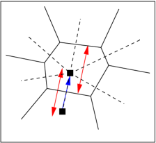
Thus, $\Delta\tau^{\mathrm{abs}}=\alpha^{\mathrm{abs}}\lambda_{\mathrm{D}}$ and, upon using Eq.12, we have $\Delta\tau^{\mathrm{abs}}=c^{\mathrm{abs}}$, which is the number of mean free paths contained in the Delaunay length $\lambda_{\mathrm{D}}$. So, if we assign a constant $c^{\mathrm{abs}}$, representing the local optical depth, to each grid point, the fraction $1-\mathrm{e}^{-c^{\mathrm{abs}}}$ of the incoming radiation is attenuated at this event centre due to absorption. Assuming that the length of a Delaunay line is much smaller than the absorption mean free path (otherwise the radiation cannot travel far), or equivalently $c^{\mathrm{abs}}\ll 1$, we can expand the exponential to first order: $1-\mathrm{e}^{-c^{\mathrm{abs}}}\approx c^{\mathrm{abs}}$.

By this, we can incorporate absorption in our method by assign a constant $c^{\mathrm{abs}}$ to each grid point, and by defining an absorption recipe:

$$I^{\mathrm{abs}} = I^{\mathrm{in}}c^{\mathrm{abs}}$$ (13)

$$I^{\mathrm{out}} = I^{\mathrm{in}}(1-c^{\mathrm{abs}}),$$ (14)

in which $I^{\mathrm{in}}$ is the amount of incoming radiation (blue arrow in Fig.7), $I^{\mathrm{abs}}$ is the amount of radiation locally absorbed, and $I^{\mathrm{out}}$ is the amount of radiation which will leave the event centre according to the scattering recipe in Fig.5. Thus, we have circumvented the inherent difficulties of the extant numerical methods (interpolating and integrating optical depths, evaluation of exponentials, etc.) and reduced the whole absorption process to the computationally efficient calculation of fractions.

We conclude by noting that $I^{\mathrm{in}}=I^{\mathrm{out}}+I^{\mathrm{abs}}$ always, by which our method is explicitly photon-conserving, in contrast to other methods which lose photons due to interpolations and other systematic errors.

3.4.2 Other processes

Of course, the recipe in Eqs.(13) and (14) can be used for various other radiation-matter interactions. If we have, for example, a mixture of two or more different gases, which have the same overall density profile, but a different mass absorption coefficient, we would have several different $c^{\mathrm{abs}}$’s assigned to each grid point, one for each type of gas.

Another useful physical process we can easily incorporate into our method is ionisation, for which we can use the local optical depth $c^{\mathrm{ion}}$ as a measure of the amount of neutral atoms at each event centre. It is important that our method is photon-conserving, because this ensures the right dimensions of a resultant Strömgren sphere, or, more accurately in an inhomogeneous medium, Strömgren region.

Furthermore, radiation that was absorbed can be re-emitted by adding it to the outgoing radiation locally, maybe even in a different frequency domain. Frequency dependence can easily be introduced by, for example, introducing an interaction matrix $A_{ij}$ which determines the redistribution of radiation $I_{i}$ from one frequency domain $i$ into radiation $I_{j}$ in another domain $j$ according to the local physical properties of the medium. These physical properties may even include complicated chemical equilibrium networks, or feedback effects from some independent hydrodynamical solver. Even Doppler effects can be taken into account.

3.5 Interaction coefficients

Now that we have shown that we can incorporate any local radiation-matter effect into our method by attaching several constants, one for each kind of interaction, to each grid point, we still have to specify how to determine the value of the constants in the set radiation-matter interaction coefficients $\{c^{i}\}$, which we assign to each grid point.

To do this, we proceed as follows: given a medium distribution profile in the form of a scalar function (or, as mentioned before, array) $\rho(\mn@boldsymbol{x})$, in which $\mn@boldsymbol{x}\in D=[0.0:1.0]^{d}$ which is the size of our $d$ dimensional computational domain, we have distributed our $N$ available grid points in such a way that it accurately samples the function $\rho^{d}(\mn@boldsymbol{x})$. Of course, we can choose our point distribution to follow a different function of the density, $f(\rho(\mn@boldsymbol{x}))$, but Eq.(12) is only valid globally with a constant $c$, when $f(\rho(\mn@boldsymbol{x}))=\rho^{d}(\mn@boldsymbol{x})$. Because Eq.(12) is valid in the whole medium, it is also valid at some location $\mn@boldsymbol{x}_{0}$ where the medium density is equal to its average density, that is at a location where

$$\rho(\mn@boldsymbol{x}_{0})=\left\langle\rho(\mn@boldsymbol{x})\right\rangle=\int_{D}\rho(\mn@boldsymbol{x})\mathrm{d}x=M_{\mathrm{tot}},$$ (15)

in which $M_{\mathrm{tot}}$ is the total mass of the medium inside the computational domain. Given the mass ‘interaction’ coefficient $\kappa^{i}$ for a certain radiation matter interaction, the mean free path at $\mn@boldsymbol{x}_{0}$ is

$$\lambda(\mn@boldsymbol{x}_{0})=1/\kappa^{i}M_{\mathrm{tot}}.$$ (16)

Because the value of the medium density at $\mn@boldsymbol{x}_{0}$ is the expectation value, the value of the grid point density at $\mn@boldsymbol{x}_{0}$ is also the expectation value. Thus, because the volume of our computational domain is unity,

$$n(\mn@boldsymbol{x}_{0})=N,$$ (17)

where $N$ is the number of available grid points, that is our resolution. As said, we know from stochastic geometry that the local Delaunay line length is determined by Eq.(8). Combining all these elements, we get

$$c^{i}=\frac{\zeta M_{\mathrm{tot}}}{N^{1/d}}\kappa^{i}.$$ (18)

Thus, given our resolution $N$ and the total mass $M_{\mathrm{tot}}$ of the medium inside our computational domain, Eq.(18) determines the global constant that we have to attach to each grid point for a certain radiation-matter interaction characterised by a mass ‘interaction’ coefficient $\kappa^{i}$.

It is, of course, possible that ${\kappa^{i}}$ is not a constant, but is a function of, for example, the local temperature. In that case, Eq.(7) is no longer generally valid and, in order to make sure that Eq.(12) still holds, we must scale the point density to the more general opacity function:

$$\rho_{\mathrm{D}}(\mn@boldsymbol{x})=\frac{\alpha^{d}(\mn@boldsymbol{x})}{\int_{D}\alpha^{d}(\mn@boldsymbol{x})}N.$$ (19)

However, we use the scaling relation Eq.(11) whenever we can, because in most cases densities are the relevant quantities obtained from hydro-solvers.

We make a final note that, if we choose a point distribution dependent on the density in a form different from Eq.(11), Eq.(12) is still valid locally, but now with a spatially varying $c^{i}(\mn@boldsymbol{x})$ in the form

$$c^{i}(\mn@boldsymbol{x})=\frac{\zeta\rho(\mn@boldsymbol{x})}{\rho_{\mathrm{D}}(\mn@boldsymbol{x})^{1/d}}\kappa^{i}.$$ (20)

Of course, it is much easier to have just one global constant $c^{i}$ for each grid point, which is why we prefer to use a point distribution in the form of Eq.(11), but this is not mandatory at all. In fact, if we were to extend our transport method to higher dimension ($d>3$), which is possible in applications beyond radiative transfer (e.g. data streams in $d$-dimensional space), the equivalent of Eq.(11) would assign too many points to just a few regions in $d$-space; in which case a varying value of $c^{i}$ would be preferable.

3.6 Resolution issues

Because we use a recipe Eq.(11), our point distribution conforms to the features of the medium density profile. Therefore, it makes no distinction between optically thin and optically thick regions, and the same recipe (variants of Eqs.(13) and (14) in combination with the scattering recipe in Fig.5) for the whole medium. But, because the contrast in medium density can, in realistic cases, be extremely high, and because this contrast is exaggerated by an exponent $d$ by using a point distribution recipe Eq.(11), we need a way to reduce the overabundant resolution in high density areas, so that we can use that part of our finite amount of available grid points $N$ in places that are undersampled.

A way of doing this is by cutting off the grid point distribution function $\rho_{\mathrm{D}}(\mn@boldsymbol{x})$ at some user-specified value, e.g. at a factor $f>1$ above the average point density, that is at $n_{\mathrm{max}}=f\left\langle\rho_{\mathrm{D}}(\mn@boldsymbol{x})\right\rangle$, and locally replace the $k$ overabundant grid points by, for example, just one. Of course, this means that the constants $c^{\prime i}$ that are to be assigned to this one point are different from the global constants $c^{i}$ as evaluated in Eq.(18). Because this point now represents $k$ separate ones, the recipe in Eqs.(13) and (14) has to be used $k$ times at this one point. So, given a global absorption constant $c^{\mathrm{abs}}$, a fraction $(1-c^{\mathrm{abs}})^{k}$ of the incoming radiation remains to be emitted. Thus, we get the same overall behaviour, if we define a new local constant $c^{\prime i}$

$$c^{\prime i}=1-(1-c^{i})^{k}.$$ (21)

If $c^{i}\ll 1$, $(1-c^{i})^{k}\approx 1-kc^{i}$, by which $c^{\prime i}\approx kc^{i}$, but this introduces a error, albeit small, so we stick to the recipe in Eq.(21).

3.7 The whole algorithm

Now that we have introduced all the basic ingredients of our new numerical method, we can describe the full recipe. Our whole simulation can be split up into $S$ individual equivalent steps, each of which consists of the following combination of ingredients:

1. Collect all the (multi-frequency) radiation that is emitted by this event centre (e.g. it is a source, or radiation is re-emitted), and all the radiation that arrives via the incoming Delaunay lines;

2. Use recipes in the form of Eqs.(13) and (14) to let this radiation interact with the medium;

3. Send out the resultant (spectrum of) radiation onto the Delaunay network according to the scheme depicted in Fig.5 until it hits the next event centre. If the emission and/or interaction is anisotropic, one can choose to distribute it onto the lines accordingly.

Starting with a list of $N$ randomly ordered grid points, we define one step as applying this list of actions once for every grid point.

Focusing on just one packet of source radiation emitted at a grid point in the middle of the computational domain, we can analytically estimate how far it will spread along the Delaunay network. Assuming that the $N$ points are distributed homogeneously and have a set of interactions coefficients $\{c^{i}\}$ attached, we can derive from basic random walk theory that after $S$ steps the second order expectation value of the displacement $\mn@boldsymbol{R}$ of the radiation packet has the form

$$\left\langle\mn@boldsymbol{R}^{2}\right\rangle=\lambda_{\mathrm{D}}^{2}S,$$ (22)

in which $\lambda_{\mathrm{D}}$ is determined by Eq.(8). Therefore, the root mean square of the net displacement is

$$\mn@boldsymbol{R}_{\mathrm{rms}}=\lambda_{\mathrm{D}}\sqrt{S},$$ (23)

Here, we have assumed that the scattering at each grid point is isotropic, but the same derivation will also hold for any scattering with front-back symmetry, as in Thomson or Rayleigh scattering.

After $S$ steps, the total intensity of the packet will have diminished by a factor $\mathrm{e}^{-S\sum_{i}c^{i}}$. If the number of steps is high enough and if the mean free path of the photon packet is large enough, the photon will reach the boundary, where it is absorbed, reflected or leaves the computational domain, depending on what kind of boundary we choose. Often, the radiation will be fully absorbed long before it reaches the boundary.

In $d$ dimensional space, the number of steps needed for the radiation packet to cover the domain, that is, to reach the boundary, is of order $O\left(N^{1/d}\right)$, and at each step the number of operations in the form of Eqs.(13) and (14) scale with the number of grid points, i.e. are of order $O(N)$, by which we expect that the simulation will have converged after an operation count of order $O\left(N^{1+1/d}\right)$. Thus, the operation count of our method is independent of the number of sources, which makes it possible to accurately simulate the radiation field of large extended sources just as rapidly as for just one or two point sources. Another thing we can conclude is that our method has a lower operation count, if the dimension $d$ is higher, but this is of no importance, because we need more points $N$ to accurately sample a higher-dimensional domain. Finally, we should mention that, if we include frequency-dependence, characterised by $N_{\nu}$, the operation count will be of order $O\left(N_{\nu}N^{1+1/d}\right)$.

4 Implementation

Having shown how our method works and what its mathematical properties are, we are in the position to show what results we get from implementing the method. We first test the method on a grid based on a Poisson point distribution, because we know that, because of Eq.(12), the homogeneous distribution is just a (special) type of inhomogeneous distribution, and the two cases are equivalent, algorithm-wise. In the next section, we will use the example of a special correlated point process which results in an inhomogeneous point distribution.

We use the algorithm described in Barber et al. (1996) to construct the Delaunay triangulation. It has been proven to perform the tessellation in $O(N\log N)$ expected time for $d\leq 3$, and in $O\left(N^{\left\lfloor d/2\right\rfloor}\right)$ expected time for fixed $d\geq 4$. The source code of an excellent and much-used implementation is freely available at http://www.qhull.org.

4.1 Point source

The first test case we used was a static point source radiating isotropically in the centre of the $[0.0:1.0]^{2}$ domain.

4.1.1 Expanding wave-front

As we have described in the previous section, at each step the radiation is split up and redistributed once at every grid point, by which the radiation can propagate only as far as one edge length along the grid. In Fig.8 we plot the logarithmic intensity of the radiation within each Voronoi cell for an increasing number of steps (note that we use an absorbing boundary). We determine the radiation within one Voronoi cell by averaging the radiation arriving, via the (on average, six) Delaunay lines, at the cell’s nucleus. The solution is scale-free, so we do not need to specify the power of the source. But we do note, that the scales next to each of the six graphs have the same maximum and minimum values.

Figure 8: Illustration of the wave-front expansion, in which a point source is used on a homogeneous grid made up of 50000 points. Shown is the logarithm of the intensity distribution after (left to right; top to bottom) 3, 9, 15, 25, 35 and 50 steps.

Comparing this process of wave-front propagation with the mathematical random walk analysis we gave in the previous section, we see that our process indeed converges to a stable solution in a finite number of steps of the order $O\left(N^{1/d}\right)$, given that $N=50000$. Indeed, we find that the difference between the result after $50$ (see Fig.8, bottom right) and $51$ steps is negligible. Thus, this implementation shows that performing several steps will make the simulation tend to the static one within polynomial time.

4.1.2 Absorption profile

We already mentioned in Section 3 that we can mimic, for example, the absorption profile by withholding a certain amount of radiation at each intersection, according to the local optical depth, or interaction coefficient, $c^{\mathrm{abs}}$. Given this test case example of a point source in the centre of our domain, we can explicitly examine how the intensity profile changes as we vary the value of $c^{\mathrm{abs}}$.

We subdivide the domain using thirty shells of equal width, concentric about the radiation source, and compute the amount of radiation within those shells for various $c^{\mathrm{abs}}$. The results for $c^{\mathrm{abs}}=0.0,0.1,..,0.8$ can be seen in Fig.9, in which the logarithm of the intensity is plotted versus the distance of the shell to the centre of the domain (of size $[0.0:1.0]^{2}$).

Figure 9: Plot of the logarithm of the intensity in each shell versus the distance of that shell to the point source for (top to bottom) $c^{\mathrm{abs}}=0.0,0.1,..,0.8$.

In the absence of absorption, the integrated radiative flux through each circle concentric about the source is constant. In order to check this, we examined the difference of the flux through adjacent circles at each step of the simulation. After a few steps, the flux became constant. In the presence of absorption, the solution to the transfer equation is (for $d\geq 1$)

$$I(r)=I_{0}\mathrm{e}^{-\alpha r},$$ (24)

in which $r$ is the distance to the point source and $\alpha$ is an absorption coefficient. Splitting up the domain in concentric circular shells as above, we may verify that the total amount of energy in each ring obeys Eq.(24). This is indeed the case.

More specifically, at a distance $r$, the amount of grid-points encountered is on average $r/l$, by which the source intensity $I_{0}$ has reduced by a factor $(1-c^{\mathrm{abs}})^{r/l}$. From elementary calculus, we know that, if the number of steps, or grid points, $r/l$ is high, we obtain

$$\lim_{r/l\rightarrow\infty}(1-c^{\mathrm{abs}})^{r/l}=\mathrm{e}^{-rc_{i}^{\mathrm{abs}}/l}=\mathrm{e}^{-r/\lambda^{\mathrm{abs}}},$$ (25)

in which we used Eq.(12) for the last equality. Thus, we see that Eq.(24) and (25) match, when the number of grid points $r/l$ or, more general, $N$ is large enough.

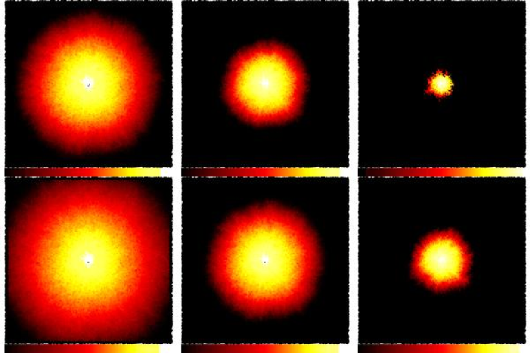
As an extra check, we computed the slopes for various values of $N$, and found that the slope indeed steepened with a factor $\left(N_{new}/N_{old}\right)^{1/d}$, as is to be expected from Eq.(18). Using more points simply leads to more absorption, as can be seen in Fig.10, in which the converged results for the same point source are plotted for $N=10000$, $N=20000$ and $N=50000$. We used the same $c^{\mathrm{abs}}$ for each one. In the $N=10000$ plot, one can still discern the individual Voronoi cells.

Figure 10: Converged results for a grid of (top to bottom) 10000, 20000, and 50000 points.

4.2 Line source

We performed all of the above tests in the case of a line source. In our case, we put the static source at the right boundary of the grid. Similar considerations as those in Subsection 4.1.2 lead us to the conclusion that the intensity profile should conform to the result Eq.(24). Because of the change of symmetry from a rotational to a mirror one, the shells should now be straight parallel strips of equal width. The remainder of the results is identical to those that are shown in Fig.9.

5 Clumpy medium distribution

Computation of the transfer of radiation as a Markov process on a Delaunay grid converges to the analytical solution, and an implementation of our method works well with several test cases.

To this, we wish to add the following considerations. First, we already stressed that one of the key issues of our method is that we make use of a stochastic point process to position the available grid points. If we construct a grid from these points, the angles between the grid lines also have a stochastic nature. In this respect, our method shares some characteristics with Monte Carlo methods. Second, if we were to increase the number of grid points to infinity, we would have enough grid points to actually sample all medium particles, and our Markov process would reduce to the actual physical one.

Another important issue is that we did not use the fact that we could enhance the accuracy obtained, when using a fixed number of points $N$, by one-dimensionally solving the transfer equations along the grid lines. As we argued in Sect. 3.2.1, we have not used this procedure for two reasons. First, because our method is computationally very efficient, we can just use a large $N$ in order to suppress the statistical noise, making the results more accurate without introducing computational complexities. Second, in the implementation presented here, the length of a grid line is of no importance for our numerical scheme. This enables us to draw the conclusion (Sect.4) that, if the results are correct in the case of a homogeneous point distribution, they will automatically be correct also in the case of a correlated distribution. Furthermore, using the scaling in Eq.(11) instead of solving the transfer equation along a Delaunay line produces an enormous speedup of the computation.

Because the length of a grid line is not used numerically, we can adjust it without changing the result, as long as we make sure that the point distribution represents the medium distribution. So, if we rescale all grid lines to the same constant length, and if we make sure that the medium rescales accordingly, such that a grid point remains attached to the same patch of medium, we do not only obtain a homogeneous point distribution, but also a homogeneous medium distribution, for which we know the method works, according to the tests in Section 4. The essential issue is that the numerical calculations to be performed on the grid will still be exactly the same as they would have been on the original grid, because of the length scale invariance. The connectivity of a ”homogenised” inhomogeneous grid will, of course, be different, but that does not influence the convergence of our method.

5.1 Correlated point processes

So far, we have only used homogeneous (Poisson) point processes, which represent homogeneous medium distributions. It is straightforward to solve the radiative transfer equations analytically in this regime of constant absorption coefficients. Using our method in this case will solve the transfer equations fast and accurately, but its performance will not differ significantly from other methods which are able to solve the transfer equation under similar conditions. The main advantages of our method are best pointed out when using a correlated point process, which mimics a clumpy medium distribution. Such clumpy distributions produce steep gradients in, for example, the absorption coefficient, when the radiation propagates outward from regions of tenuous medium to dense regions with a very high opacity. It is in this regime, in which it is impossible to find an exact analytical solution to the transfer equations, that it will be difficult and computationally costly to use the regular numerical schemes as discussed in Section 2.2 for solving the equations. Each one needs a superimposed grid, and because the size of a grid cell should be small enough to obtain the accuracy to resolve the rapidly varying density properties of the medium, a huge amount of storage and CPU-power is needed, even for the tenuous regions where less spatial coverage is needed.

In the previous section, we pointed out that our method solves the radiative transfer equation for every point distribution using the same simple Markovian random walk process. In this section, we will exploit this fact and we will use a correlated point process representing a clumpy medium distribution to demonstrate the optimal resolution and speed efficiency of our method.

5.2 Fractal point process

There are many ways to define a correlated point process, but for this paper we use a fractal point process to generate the clumpy point distribution. There are a number of reasons for this choice, the most important ones being that the process has a simple mathematical definition and a straightforward implementation, and that its statistical properties are scale-free by definition, which makes the conclusions we will draw about the statistics of the resultant tessellation more general.

Fractal (stochastic) point processes have been widely used as a modelling tool (for a review, see Lowen & Teich, 1995). In particular, Mandelbrot (1982) used it to model a non-standard random walk resulting in a linear Lévy dust which, he showed, could be used to model galaxy clusters. Because of this feature, we will use a modified version of his recipe for constructing the correlated point process, which we will now describe.

A Lévy flight is a sequence of flights separated by stopovers. It is constructed by choosing the first stopover randomly and starting the flight from that point. The (straight-line) flights have the following properties: their direction is random and isotropic, the different flights are statistically independent (thus, the Lévy flight is a Markov process), and their lengths follow a probability distribution

$$f(r)=kr^{d-1-D}=kr^{1-D},$$ (26)

where $d$ is the dimension of the space in which the flights occur (in our case, $d=2$), $k$ is a normalisation constant, and $D$ is the fractal dimension as defined in Mandelbrot (1982). Eq.(26) is a modification of the distribution function used in Mandelbrot (1982) to the effect that the clustering of points around $r=0$ is avoided. Thus, if $D=0$, we obtain the regular Poisson point process, and if $D>0$, we have an exponential decaying distribution function, which is scale-free as should be expected from a fractal distribution. Clustering will increase, when $D$ is increased. It is only the stopovers we are interested in, because they will be the points of the resultant fractal point process. The process is scale-free and Markovian, by which it is allowed to rescale and translate the resultant point distribution, so as to center and fit it in our $[0.0:1.0]^{2}$ domain, without altering the statistical properties.

Of course, we have to choose a lower and upper bound ($A$ and $B$, respectively) for $r$. Thus, we obtain for the flight-lengths the cumulative distribution function

$$F(r)=\frac{r^{2-D}-A^{2-D}}{B^{2-D}-A^{2-D}}.$$ (27)

We fix the upper bound $B$ (the maximum flight length) as half the width our domain and choose the lower boundary $A$ to be two orders of magnitude smaller. Thus,

$$r\in\left[0.01,0.5\right].$$ (28)

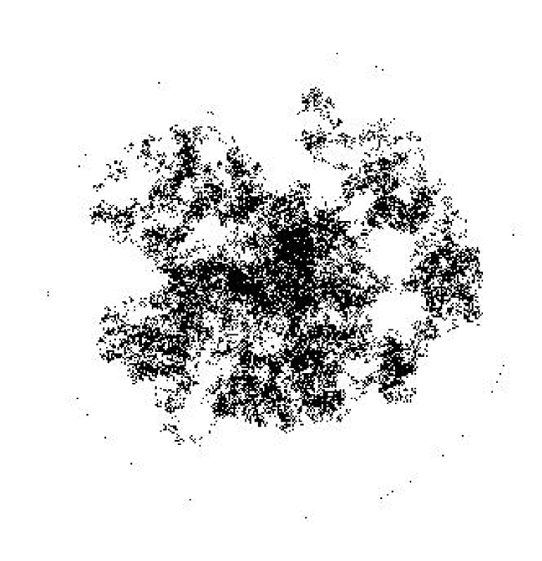
An example of this process satisfying Eq.(27) and (28), with $D=0.5$ and $N=10^{5}$, is shown in Fig.11. We will use this point distribution to illustrate our transfer method in Section 5.4.

Figure 11: Fractal point process satisfying (27) and (28) with fractal dimension $D=0.5$ for $N=10^{5}$ points. The dots around the fractal distribution are boundary points, obtained by randomly placing 100 points on the circumference of a circle with radius 1.1

5.3 Length-angle correlation

The point distribution, which is a result of the fractal point process as defined in the previous, gives us the opportunity to assert our claim in Subsection 3.3 that the angle between two long Delaunay lines is, on average, smaller than the one between two short lines, by which the angular resolution is higher for radiation being emitted into optically thin media, which is just what is needed. Given a point distribution, it is almost always impossible to find an exact distribution function $g(\lambda_{\mathrm{D}},\theta)$ for the correlation between the Delaunay edge length $\lambda_{\mathrm{D}}$ and the corresponding angle $\theta$, so in order to find the expectation value for the amount of deflection given a certain length of the Delaunay line, we do a simple Monte Carlo experiment using a fractal point process, the result of which is quite general, because the fractal point process is scale-free.

We construct a point distribution by using the same recipe as used for making the result in Fig.11, but now we use $N=2\cdot 10^{5}$ points and define the periodic boundary conditions $x=x-\left\lfloor x\right\rfloor$ and $y=y-\left\lfloor y\right\rfloor$. The periodic boundary conditions will result in a distortion of the statistical properties of the resultant tessellation, because of the overlapping parts of the Lévy flight, but the overall statistical behaviour on small scales will still have the fractal properties.

At each grid point, we order the connected Delaunay lines of the resultant triangulation clockwise. Evaluating the average length between two neighbouring lines of these two lines as well as the angle between them, we can make a statistic of the length-angle correlation. We sample the lengths by using $20$ bins going from length $0$ up to the maximum edge-length (within the triangulation) and the angles by using $50$ bins in the range $\left[0,2\pi\right]$. In this way we can plot a (normalised) distribution function for the angle for each edge-length bin. The result for several length-bins can be seen in Fig.12. The lines were made using Bézier curves (see Bartels et al., 1998) so as to approximate the trend of the data-points. Using these Bézier curves is justified, because we are only concerned with the trend, or overall behaviour, and not with very accurate quantitative results. We should remark, that the distribution functions do go to zero as is required, we would just have to put more angle-bins near zero. It is interesting to note the high values of the distribution functions near zero. With a normal Poisson distribution, the distribution function is $f(\theta)=\frac{4\sin\theta}{3\pi}\left((\pi-\theta)\cos\theta+\sin\theta\right)$ (e.g Van de Weygaert, 1991), which decreases monotonically when approaching $\theta=0$, so, apparently, the introduction of a (fractal) correlated point process introduces a large amount of small angles.

Figure 12: Plot of the (normalised) probability functions for the angle between the two most straightforwards paths for the bins of lengths 0.1, 0.2, … ,0.6 times the maximum length.

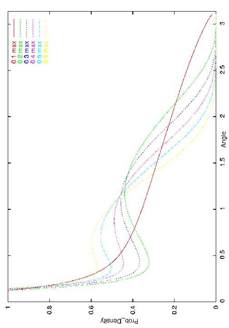
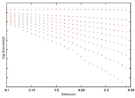
One can readily see that, when the average edge-length is increased, the average angle between the two lines will, on average, be smaller. This is noticeable when plotting the expectation value of the angle versus the length in Fig.13. There is a clear downward trend, with more scatter towards higher lengths because of the statistical noise. We simply have more data-points at shorter lengths.

Figure 13: Plot of the expectation value of the angle (in radians) versus the (average) length of the lines.

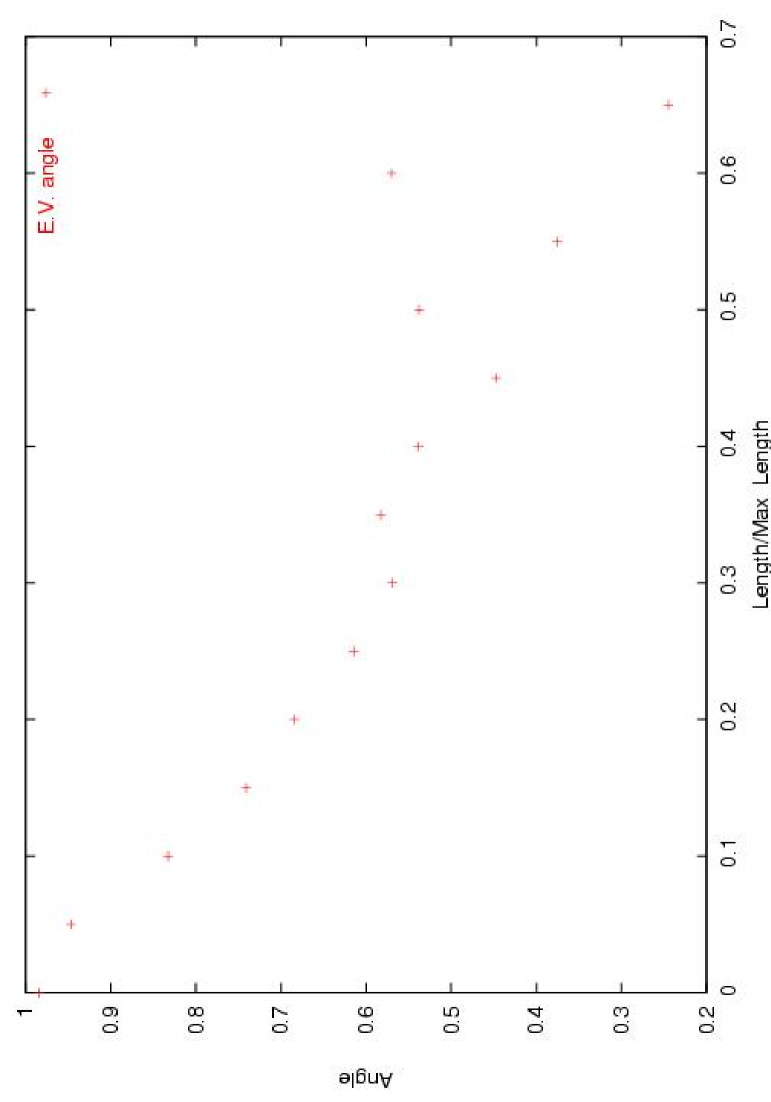
Thus, we can conclude that the angle between two long Delaunay lines (which both originate at the same grid point) will be smaller if the average edge-length is longer. This is a highly advantageous property of the Delaunay tessellation based on a correlated point process. Radiation propagating outwards from a dense region into a tenuous medium will move onto longer Delaunay lines which connect dense regions. This means that the angular resolution will be high, as it should be in those regions.

5.4 Application

We will now show the results of the application of our radiative transfer method used on a grid based on a correlated, fractal, point process. We use the same point distribution as in Fig.11, and we put a point source, radiating statically, in the middle of our $[0.0:1.0]^{2}$ domain. We assign a constant amount of absorption $c^{\mathrm{abs}}$ to each vertex, and to unambiguously define an absorbing border we randomly (uniform distribution) place $100$ extra points on the circumference of a circle with radius $r=1.1$ (see Fig.11).

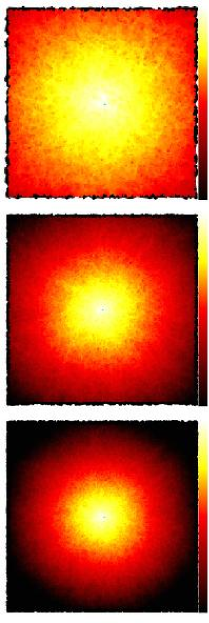
The converged results for $c^{\mathrm{abs}}=0.0500$, $0.0375$, $0.0250$ and $0.0125$ (we need small $c^{\mathrm{abs}}$’s, because there is a huge amount of points) are plotted in Fig.14. One should note that the intensity is plotted on a logarithmic scale, by which it is scale-free.

Figure 14: Plot of the logarithm of the intensity of the converged results for (top) $c^{\mathrm{abs}}=0.0500$ and $c^{\mathrm{abs}}=0.0375$, and (bottom) $c^{\mathrm{abs}}=0.0250$ and $c^{\mathrm{abs}}=0.0125$. Note the shadows behind the dense clumps, especially in the bottom left image.

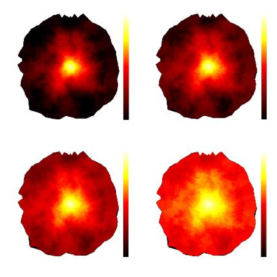
Comparing Fig.14 with the point distribution in Fig.11, one immediately sees that the method works beautifully. All the features of the point distribution stand out clearly in the radiation results. One readily points out the high and low density regions, and because of the high resolution ($N=10^{5})$, the distinct features of the high density regions are resolved very accurately. The exact simulation of shadowing effects is exemplified, when increasing the absorption coefficient $c^{\mathrm{abs}}$. With $c^{\mathrm{abs}}=0.0500$, we clearly see the radiation escaping in the directions of the lowest point density.

The extremely high resolution is pointed out more efficiently, when zooming in on a part of the domain. Defining the left-bottom corner of the $c^{\mathrm{abs}}=0.0500$ result in Fig.14 as $(0,0)$ and the top-right one as $(1,1)$, we zoom in on the region $x,y\in\left[0.25,0.50\right]$ and plot the point distribution and radiation result in Fig.15. Notice the large size of the Voronoi cells filling up the voids in the point distribution. Even now, the resolution in the dense region is still high enough to obtain a high amount of accuracy.

Figure 15: Magnified portion $x,y\in\left[0.25,0.50\right]$ of Fig.11 (left) and Fig.14 (right) with $c^{\mathrm{abs}}=0.0500$.

6 Completing the method

We have shown that our method solves the radiative transfer equations without much numerical effort, even in those cases in which the medium is highly inhomogeneous. It is in these cases that our method stands out from other radiative transfer methods, which have difficulties when passing from one opacity regime to another.

There is one complication, however, as we pointed out earlier in Section 3, because we treat each event centre as a scattering centre. When our simulation domain contains large regions of (almost) transparent medium, i.e. when $\lambda^{\mathrm{scat}}$ becomes bigger than or comparable to the dimensions of our domain, we can immediately see that this results in an undersampling. An extreme example is that of an empty (optically inactive) domain, in which our method dictates that no points should be used, by which we do not have a grid along which the radiation can propagate. A less extreme example is that of a region of almost empty (and, thus, undersampled) space behind a highly absorbing clump of matter, in which we would like to resolve the sharp shadow cast by the clump. In both cases the sought-after results are just straight-line trajectories, which are the solutions of the transfer equations for radiation propagating through a vacuum.

We will now present a supplement to our method, which will enable us to solve the radiative transfer equations in these cases on the same kind of unstructured grid based on a Delaunay tessellation.

6.1 Long characteristics

Let us focus on the example of a simulation domain which is totally devoid of optically active medium. Because we need for a grid solving the equations, we proceed by creating a point distribution. Because the matter is distributed homogeneously across the domain (it is homogeneously empty), we choose a Poisson point process to generate our point distribution. The amount of points we choose may vary from case to case and will depend on the total amount of points available.

Because the solution of the transfer equation in this regime is a superposition of straight line trajectories and because now each grid point does not represent a packet of matter at which photons get scattered, we need to modify our photon propagation scheme as described in Section 3, in such a way that it works according to the long characteristics principle, as laid out in Subsection 2.2. In order to accommodate this requirement, we reject the Markov assumption as introduced in Section 3, and we do not scatter the radiation at each grid point, but we keep track of its original direction, which is now a very relevant quantity.

Therefore, we make the modification to the transfer scheme as laid out in Section 3 that at each intersection we choose the $d$ most straightforward paths with respect to the original direction (see Fig.16). We discuss later why we choose to split up the radiation into $d$ parts.

Figure 16: The advection scheme, as originally laid out in Section 3, is modified in such a way that at each grid point the radiation is split and redistributed amongst the $d$ Delaunay lines which are most ‘straightforward’ with respect to the original direction (blue dashed line) of the radiation packet.

6.1.1 Mathematical analysis

Figure 17: One possible path of a radiation packet performing a walk of $n$ steps on the Delaunay graph. The $i$-th step is parametrised by an angle $\theta_{i}$, with respect to the original direction $x$.

For a mathematical analysis of the expectation values of the position of a photon packet in this modified scheme, we proceed as follows. An example of a path of a photon packet performing a walk in two dimensions is given in Fig.17. The following analysis, however, will be valid in $d$-dimensional space.

Because of cylindrical symmetry around the original direction $\mn@boldsymbol{x}$, we can parametrise the $i$-th step by only one angle $\theta_{i}$, which is the angle between the $i$-th Delaunay edge and the original direction. Thus, the expectation value of the total displacement $\mn@boldsymbol{R}_{n}=\mn@boldsymbol{r}_{1}+...+\mn@boldsymbol{r}_{n}$ is

$$\left\langle\mn@boldsymbol{R}_{n}\right\rangle = \left\langle\mn@boldsymbol{r}_{1}\right\rangle+...+\left\langle\mn@boldsymbol{r}_{n}\right\rangle$$ (29)

$$= {n}\lambda_{\mathrm{D}}\left\langle\cos\theta\right\rangle\frac{\mn@boldsymbol{x}}{\left|\mn@boldsymbol{x}\right|}$$

$$= {n}\lambda_{\mathrm{D}}\chi\frac{\mn@boldsymbol{x}}{\left|\mn@boldsymbol{x}\right|},$$

in which $\lambda_{\mathrm{D}}$ is defined in Eq.(8), and

$$\chi=\int^{\pi}_{-\pi}h(\theta)\cos\theta\mathrm{d}\theta.$$ (30)

$h(\theta)$ Is a certain symmetric function, which characterises the probability distribution of the angle $\theta$ and which, in most cases, cannot be evaluated analytically. The second-order expectation value can be evaluated as follows:

$$\left\langle\mn@boldsymbol{R}^{2}_{n}\right\rangle = \left\langle\mn@boldsymbol{r}^{2}_{1}\right\rangle+\left\langle\mn@boldsymbol{r}_{1}\cdot\mn@boldsymbol{r}_{2}\right\rangle+...+\left\langle\mn@boldsymbol{r}^{2}_{n}\right\rangle$$ (31)

$$= \lambda_{\mathrm{D}}^{2}\left({n}+{n}({n-1})\left\langle\cos(\theta_{i}+\theta_{j})\right\rangle\right),$$

in which we may choose $i$ and $j$ randomly from the set $\left\{1,...,n\right\}$, as long as $i\not=j$, because the distribution function $h(\theta)$ has the same form for each angle $\theta_{i}$. Using the cosine addition formula, we can reduce Eq.(31) to

$$\left\langle\mn@boldsymbol{R}^{2}_{n}\right\rangle=\left({n}+{n}({n-1})\chi^{2}\right)\lambda_{\mathrm{D}}^{2}.$$ (32)

Thus, the variance of the displacement is

$$\sigma^{2}_{\mn@boldsymbol{R}_{n}}={n}\lambda_{\mathrm{D}}^{2}(1-\chi^{2}).$$ (33)

If $h(\theta)\propto\delta(\theta)$, then $\chi=1$, by which $\left\langle\mn@boldsymbol{R}_{n}\right\rangle=\lambda_{\mathrm{D}}{n}\frac{\mn@boldsymbol{x}}{\left|\mn@boldsymbol{x}\right|}$ and $\sigma^{2}_{\mn@boldsymbol{R}_{n}}=0$ as should be expected. The exact form of a distribution function like $h(\theta)$ can probably not be evaluated, even in the well-studied Poisson case, but we can use a step function as an approximation. Thus, given that in 2D the average number of Delaunay lines meeting at a grid point is $6$, we use as a step function $h(\theta)=3/\pi$ on the domain $\theta\in[-\pi/6,\pi/6]$. This results in $\chi=3/\pi$, by which

$$\left\langle\mn@boldsymbol{R}_{n}\right\rangle=\frac{3n\lambda_{\mathrm{D}}}{\pi}\frac{\mn@boldsymbol{x}}{\left|\mn@boldsymbol{x}\right|},$$ (34)

which is very close (difference of less than $5\%$) to the distance along a straight line, which would be $n\lambda_{\mathrm{D}}$. We can always, of course, rescale the lengths so as to make sure that the distance traversed equals the exact physical one. More importantly, the variance in the displacement, in this case, is

$$\sigma^{2}_{\mn@boldsymbol{R}_{n}}=\frac{\pi^{2}-9}{\pi^{2}}\lambda_{\mathrm{D}}^{2}{n}.$$ (35)

We know that the results of using a step-function as distribution function gives upper bounds on the values of Eq.(29) and Eq.(33), because the actual distribution function would peak around $\theta=0$ and would decrease as $\left|\theta\right|$ increases, so we expect the actual value of $\sigma^{2}_{\mn@boldsymbol{R}_{n}}$ to be smaller. Thus, we can simulate a straight line trajectory with this method, because $\mn@boldsymbol{R}_{n}\propto{n}\mn@boldsymbol{x}$, but, still, the standard deviation will increase with $\sqrt{n}$.

What is more important is the behaviour of the standard deviation, if the number of grid points $N$ increases. Let us therefore examine a line segment in the simulation domain of length $L$ ($\leq\sqrt{d}$, if we have a $[0.0:1.0]^{d}$ domain). Because the point distribution is homogeneous, we can conclude that the number of steps to cover the line is

$${n}=\xi{N}^{1/d},$$ (36)

in which $\xi\leq\frac{\pi}{3}\zeta\sqrt{d}$, which can be found by using the upper bound Eq.(34) and the Eq.(8) for the length $\lambda_{\mathrm{D}}$ of a Delaunay line. If we combine Eq.(35) with Eq.(36), again using Eq.(8), we obtain

$$\sigma\propto\lambda_{\mathrm{D}}\sqrt{n}\propto{N}^{-1/2d}.$$ (37)

Thus, we can conclude that the amount of widening of the beam will go to zero, if we increase the amount of grid points $N$.

Even if we do not have a large amount of points to suppress the widening of the beam, we have another effect which compensates for the widening. Namely, at each intersection the radiation is split up into $d$ parts. This means that the intensity at points farther away from the straight line trajectory is much less than at points close by, simply because of the fact that more paths cross each other at points close to the line.

6.1.2 Implementation

There are several easy algorithms to numerically simulate a straight line across a Delaunay graph, most having their origin in mobile telecommunications (see Baccelli et al., 1998). These algorithms determine the shortest path along a Delaunay-graph from one point to another, both of which lie on a line. So, why not use one of these algorithms, which can be implemented into our method without much effort, to accurately model a straight line, instead of using the one we described which introduces a minor widening of the beam?

The main reason is that, when we have a point source, there are only so many rays, or Delaunay edges, emerging from that point source. This means that parts of the volume at large distances from the source are largely undersampled, with only a couple or none of the rays intersecting it. This is the main drawback of the usual methods which we criticised in Section 2. Therefore, we still use the feature of our scheme, that we split up the radiation at each intersection into $d$ parts. This introduces a $\sqrt{n}$ widening of the beam, but it also makes sure that the whole domain will be covered. In this sense, it shares some of the characteristics of the adaptive ray tracing mechanism as described in Abel & Wandelt (2002), which describes a way of splitting up rays, so as to accurately sample the whole domain, but, by doing so, also introduces a similar widening of the beam.

Another reason is that unless the low density regions are extremely big, the region in which one might want to use this long characteristics method is not very large, so the effect of beam widening is not of much importance, even if we only have a small number of points, because the number of steps $n$ is small.

To get an idea of the algorithm and how it works, we try to simulate a laser beam in a transparent medium. We use a Poisson process to create a homogeneous point distribution of $3\times 10^{4}$ and $10^{5}$ points and place a pencil beam in the domain. The result can be seen in Fig.18. Note that the absorption coefficient is equal to zero.

Figure 18: Results of using the long characteristics version of our method in order to simulate a pencil beam, using 30000 (top) and 100,000 points (bottom). The absorption coefficient is equal to zero.

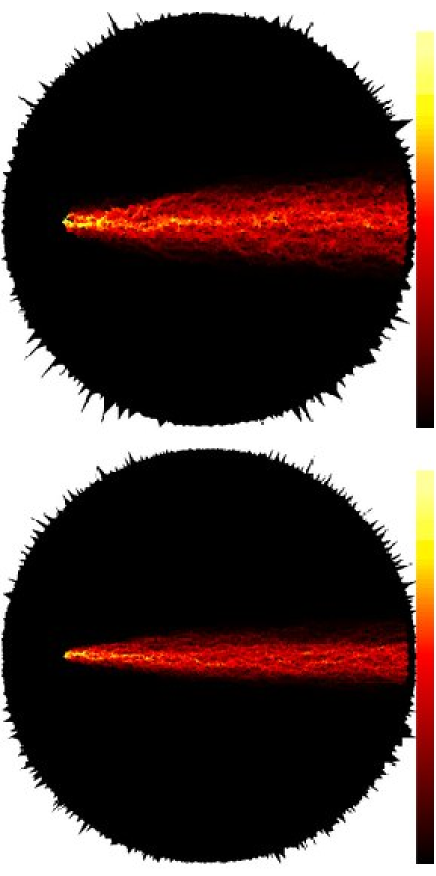
As expected, the beam is narrower when the number of points is larger, as should be expected from Eq.(37), and the intensity is highest close to the straight line trajectory.

Figure 19: Radiation from a point source hitting a highly absorbing square, which casts a sharp shadow. Result obtained by using the long characteristics variant with $10^{5}$ points, homogeneously distributed.

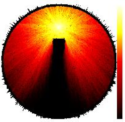
These properties make this variant ideal to resolve sharp shadows behind highly absorbing objects. To illustrate this, we simulate a point source by defining all points within a circle of radius $0.1$ with $(0.5,0.8)$ as a centre to be point sources, and we put a highly absorbing object in front of our source. The object, in this case, is a square with side $0.1$ which is centred on $(0.5,0.65)$, with $c^{\mathrm{abs}}=1.0$ at each point. The rest of the domain (except the absorbing boundaries, of course) has $c^{\mathrm{abs}}=0.1$. The result for $10^{5}$ points is plotted in Fig.19.

6.2 Usage

As we have shown in the previous subsection, the long characteristic variant of our method results in numerical solutions in which shadows can be resolved quite accurately. So, why do we not use this long characteristic variant as our main method to solve the radiative transfer equation numerically? There are several reasons.

First, the long characteristic variant is only useful when there are large, almost empty regions, in which there would be no scattering. Because the biggest difficulty lies in solving the equation for photons propagating through media of various densities, we have made sure that the core of our method solves this difficult problem. The second issue is speed. The improved angular resolution of this variant does not come without a cost. For $i$ point sources, the method will in 2D be $6i$ (on average $6$ Delaunay-edges per nucleus) times slower than with the original method, which has an operation count of $O(N)$ independent of the number of sources.

Thus, we have presented two methods (excluding the long characteristics variant from Baccelli et al., 1998) which are able to solve the transfer equations on unstructured grids, such as a Delaunay graph. Each has its own advantages and disadvantages and it is basically up to the user to choose which version is most suited for the problem at hand.

For now, we will choose to use the first version of our method as a basis, making use of its speed, efficiency and adaptability to solve the transfer equation, when it is most difficult to solve, and we shall only resort to the slower long characteristics variant in those cases where there are large transparent regions, or in which high resolution shadows are needed.

7 Conclusions and future work

We have presented a new numerical method that is able to solve the transfer equation efficiently on unstructured grids, such as a Delaunay graph, which are based on random point processes. One of its main advantages is that it uses a Lagrangian grid, which puts the accuracy where it is needed, and it automatically puts, as we have shown, the angular resolution where it is needed. We have shown that if we choose a point distribution in the from of Eq.(11) to mimic the medium density profile, we obtain a set of global constants, or interaction coefficients $\{c^{i}\}$, which are assigned to each grid point, or event centre. This procedure ensures that, when the radiation performs a Markovian random walk along the graph from one event centre to the next, the overall macroscopic behaviour of the radiation field is just as we expect from the radiative transfer equations. One can intuitively understand this, because, if we assign the same amount of withheld radiation $c^{i}$ to each grid point and we put more points where the medium is more dense, that region will automatically become more opaque. Moreover, because the point distribution adapts to the medium distribution and because the algorithm makes no distinction between optically thick and optically thin regions, our new method can be used equally as well in every opacity regime, which makes this method particularly suitable to be used in those realistic cases, where the medium passes from one regime to the next. It is in these cases that most other methods fall short. But the most important advantage of all is that we have reduced the complex system of coupled differential equations to a simple one-dimensional random walk on a graph, in which the interaction recipes in the form of Eqs.(13) and (14) are the most difficult calculation to be performed. Therefore, the method solves the transfer equation in $O\left(N^{1+1/d}\right)$ operations, in which $N$ is the number of resolution elements, or grid points, even in the cases where the number of sources approaches $N$, for which the operation count of other $O(N)$ schemes (e.g. Abel et al., 1999) increases towards higher orders. This makes our method extremely suitable for use in cases with large extended sources distributed over space. Any such implementation will therefore be extremely fast.

We have also described a supplement to our method, which can be used, if the domain contains large almost empty regions, by which it would be highly undersampled. This long characteristics variant can be used to accurately resolve shadows behind highly absorbing objects, but it comes with a cost. When the number of sources is increased to $N$, the operation count will increase to $O(N^{2})$.

There are several things that remain to be done and on which we are working already. First, we are extending our method to three dimensions. This is no problem, because our code is set up generically and the mathematical analysis is valid for $d$-dimensional space. Another thing is that we have not incorporated feedback from the medium at all. We want to apply our method to cases in which the medium is optically active and the source function is inhomogeneous and frequency-dependent, or which incorporates ionisation, recombination and photodissociation. That is, we want to incorporate a wider variety of interaction coefficients $\{c^{i}\}$. A most promising feature of our method is that it also inherently solves the time-dependent radiative transfer equations without doing any extra work. Because our method is photon-conserving, we can use the time-dependent variant, for example, to accurately model ionisation fronts expanding in an inhomogeneous medium. Finally, it is our aim to combine our method with the SPH method, or even other hydrodynamical schemes, so that we can combine the two essential parts of the physics which probably governs the formation of most structures in our universe.

References

- Abel et al. (1999) Abel, T., Norman, M. L. & Madau, P. 1999, ApJ, 523, 66
- Abel & Wandelt (2002) Abel, T. & Wandelt, B. D. 2002, MNRAS, 330, L53-L56
- Baccelli et al. (1998) Baccelli, F., Tchoumatchenko, K. & Zuyev, S. 1998, Markov Paths on the Poisson-Delaunay Graph, INRIA Rapports de Recherche, Nr. 3420
- Barber et al. (1996) Barber, C. B., Dobkin, D. P. & Huhdanpaa H. 1996, ACM Transactions on Mathematical Software, 22, No. 4, 469-483
- Bartels et al. (1998) Bartels, R. H, Beatty, J. C. & Barsky, B. A. 1998, Bézier Curves, Ch. 10 in An Introduction to Splines for Use in Computer Graphics and Geometric Modeling, San Francisco, CA: Morgan Kaufmann, pp. 211-245, 1998
- Chandrasekhar (1943) Chandrasekhar, S. 1943, Rev. Modern Phys., 15, 1-87
- Delaunay (1934) Delaunay, B. 1934, Classe des Sciences Mathématiques et Naturelles, 7, 793
- Duderstadt & Martin (1979) Duderstadt, J. J. & Martin W. R. 1979, Transport Theory, John Wiley and Sons, New York
- Greengard (1988) Greengard, L. F. 1988, The Rapid Evolution of Potential Fields in Particle Systems, MIT Press
- Kunasz & Auer (1988) Kunasz, P. B. & Auer, L. 1988, JQSRT, 39, 67
- LeVeque (1998) LeVeque, R. J., Mihalas, D., Dorfi, E. A., et al. 1998, pp. 104-111 in: Computational Methods for Astrophysical Fluid Flow, Saas-Fee Advanced Course 27, eds. O. Steiner & A. Gautschy, Springer Verlag, Berlin
- Lowen & Teich (1995) Lowen, S. B. & Teich, M. C. 1995, Fractals, 3, No. 1
- Lucy (1977) Lucy, L. B. 1977, AJ, 82, 1013
- Mandelbrot (1982) Mandelbrot, B. B. 1982, The Fractal Geometry of Nature, W. H. Freeman & Co.
- Mihalas et al. (1978) Mihalas, D., Auer, L. & Mihalas, B. 1978, ApJ, 220, 1001
- Monaghan (1992) Monaghan, J. J. 1992, ARA&A, 30, 543
- Okabe et al. (2000) Okabe, A., Boots, B., Sugihara, K., & Chiu, S.N. 2000, Spatial Tessellations: Concepts and Applications of Voronoi Diagrams, 2nd Ed., Chichester, John Wiley & Sons Ltd
- Pelupessy et al. (2003) Pelupessy, F. I., Schaap W. E. & Van de Weygaert, R. 2003, A&A, 403, 389
- Rutten (1999) Rutten, R. 1999, Radiative Transfer in Stellar Atmospheres, http://www.fys.ruu.nl/~rutten/
- Schaap & Van de Weygaert (2000) Schaap, W. E., & Van de Weygaert, R. 2000, A&A, 363, L29
- Steinacker et al. (2002) Steinacker, J., Hackert, R. & Steinacker, A. 2002, JQSRT, 74, 183
- Stoyan et al. (1996) Stoyan, D., Kendall, W. S. & Mecke, J. 1996, Stochastic Geometry and its Applications, 2nd Ed., John Wiley & Sons
- Van de Weygaert (1991) Van de Weygaert, R., Voids and the Geometry of Large Scale Structure, Ph.D. Thesis, Leiden 1991
- Voronoi (1908) Voronoi, G. 1908, Journal für die Reine und Angewandte Mathematik, 134, 198