Flares from small to large: X-ray spectroscopy of Proxima Centauri with XMM-Newton

We report results from a comprehensive study of the nearby M dwarf Proxima Centauri with the XMM-Newton satellite, using simultaneously its X-ray detectors and the Optical Monitor with its U band filter. We find strongly variable coronal X-ray emission, with flares ranging over a factor of 100 in peak flux. The low-level emission is found to be continuously variable on at least three time scales (a slow decay of several hours, modulation on a time scale of 1 hr, and weak flares with time scales of a few minutes). Several weak flares are characteristically preceded by an optical burst, compatible with predictions from standard solar flare models. We propose that the U band bursts are proxies for the elusive stellar non-thermal hard X-ray bursts suggested from solar observations. In the course of the observation, a very large X-ray flare started and was observed essentially in its entirety. Its peak luminosity reached $3.9\times 10^{28}$ erg s^-1 [0.15–10 keV], and the total X-ray energy released in the same band is derived to be $1.5\times 10^{32}$ ergs. This flare has for the first time allowed to measure significant density variations across several phases of the flare from X-ray spectroscopy of the O vii He-like triplet; we find peak densities reaching up to $4\times 10^{11}$ cm^-3 for plasma of about $1-5$ MK. Abundance ratios show little variability in time, with a tendency of elements with a high first ionization potential to be overabundant relative to solar photospheric values. Using Fe xvii lines with different oscillator strengths, we do not find significant effects due to opacity during the flare, indicating that large opacity increases are not the rule even in extreme flares. We model the large flare in terms of an analytic 2-Ribbon flare model and find that the flaring loop system should have large characteristic sizes ($\approx 1R_{*}$) within the framework of this simplistic model. These results are supported by full hydrodynamic simulations. Comparing the large flare to flares of similar size occurring much more frequently on more active stars, we propose that the X-ray properties of active stars are a consequence of superimposed flares such as the example analyzed in this paper. Since larger flares produce hotter plasma, such a model also explains why, during episodes of low-level emission, more active stars show hotter plasma than less active stars.

1 Introduction

Coronal energy release on magnetically active cool stars is, according to current understanding, largely driven by the interplay of surface convective motion and magnetic fields anchored in the star’s outer convection zone. Strong variability in coronal emissions due to flares (in X-rays, the extreme ultraviolet, or the radio range) support theories proposing magnetic instabilities as the main drivers of energy release and transport (see Haisch et al. 1991 for a general multi-wavelength review of solar and stellar flares). Although stellar coronal radiation has traditionally been classified as “quiescent” or “flare” depending on the recorded time scale of variability, recent studies have cast some doubt on the overall meaning of this distinction for magnetically very active main-sequence stars. First, sensitivity limitations inevitably smooth out low-level variability. Second, a superposition of many strongly overlapping flares tends to produce smooth light curves in particular for statistical distributions of flare energies for which the low-energy population dominates the total energy budget (Kopp & Poletto 1993, Güdel 2000). And third, long time series monitoring stellar X-ray or EUV activity have provided evidence for continuous variability ascribed to flares, to an extent that possibly all of the observed coronal emission can be attributed to explosive energy release (Audard et al. 2000, Kashyap et al. 2002, Güdel et al. 2003a). This latter hypothesis is presently also in the center of solar coronal research (e.g., Porter et al. 1995, Krucker & Benz 1998, Parnell & Jupp 2000, Aschwanden et al. 2000) in the context of “micro-” or “nano-”flares.

Large, outstanding coronal flares may thus be the prototypes of the coronal heating agents accessible relatively easily by monitoring programs available on X-ray satellites. Their investigation may provide the fundamental parameters required to understand explosive energy release by magnetic reconnection, shed light on the magnetic geometry prevailing in stellar flares, and help understand processes transporting chromospheric and photospheric material into the corona. Comparing such studies on magnetically active stars with solar findings is particularly important as magnetic processes on the former may fundamentally differ from those on the Sun, given the much larger filling factor of surface magnetic fields on active stars. XMM-Newton and Chandra offer a new dimension to stellar flare research by providing access to highly sensitive high-resolution X-ray spectroscopy, thus potentially revealing information not only on the temperature structure but also on electron densities, turbulence, or bulk mass motions.

During a recent XMM-Newton campaign on the nearest star to the Sun, Proxima Centauri, we were fortunate in recording a major long-duration X-ray and optical flare that outshone the average pre-flare emission by almost two orders of magnitude in X-rays, and several magnitudes in the optical. Early findings from this campaign are described in Güdel et al. (2002a = Paper I). The observing program was initially devised to investigate the statistics of low-level activity, providing access to the weakest flares yet on any star other than the Sun. The campaign indeed recorded a sequence of low-level flares to an extent that no part of the light curve can be described as steady, for a duration of about 35 ks (Paper I). Many X-ray events were characteristically preceded by optical bursts in a manner predicted by the chromospheric evaporation scenario (Antonucci et al. 1984, Dennis 1988, Hudson et al. 1992). The large flare for the first time provided a sufficient statistical signal-to-noise ratio to explicitly and significantly measure the run of electron densities in the flare plasma from spectroscopic He-like line triplets. Electron densities of several times $10^{11}$ cm^-3 were found during peak time, while they rapidly decreased during the flare decay phase. These observations compare favorably with previous solar spectroscopic measurements of flare densities (McKenzie et al. 1980, Doschek et al. 1981).

The present paper presents the complete XMM-Newton data set on Proxima Centauri and discusses some models for the large flare. In a companion paper (Reale et al. 2004), we will present a series of hydrodynamic simulations for the same flare. The paper is structured as follows: Sections 2 and 3 describe the target and the observations, Sect. 4 presents the analysis and our results, while Sect. 5 discusses the findings in the context of flare physics and coronal heating. Sect. 6 contains our conclusions.

2 The Target

Proxima Centauri is a magnetically active dM5.5e dwarf ($V=11.05$, see SIMBAD database; $L_{\rm bol}=6.7\times 10^{30}$ ergs^-1, see Frogel et al. 1972) revealing strong coronal activity. At a distance of $1.295\pm 0.005$ pc (Perryman et al. 1997), it is the closest star to the Sun. Its “quiescent” X-ray luminosity $L_{\rm X}\approx(4-16)\times 10^{26}$ erg s^-1 (Haisch et al. 1990) is similar to the Sun’s despite its $\approx$50 times smaller surface area. It has attracted the attention of most previous X-ray observatories. Haisch et al. (1980) and Haisch et al. (1981) observed quiescent and flaring X-ray emission from this star with the Einstein satellite, with the largest flare reaching an X-ray luminosity of $L_{\rm X}=7.4\times 10^{27}$ erg s^-1 and peak temperatures of 17 MK during the rise to the luminosity peak. The surface filling factor of X-ray emitting magnetically confined plasma was estimated to be about 20% based on solar analogy. Interestingly, coordinated radio, optical, and ultraviolet observations recorded no flare emissions. The authors interpreted this long-decay flare (decay time scale $\tau\approx 20$ min) by a series of arches cooling predominantly by radiation, with dimensions comparable to the stellar radius. In a follow-up observation, Haisch et al. (1983) report another very large flare, with a peak X-ray luminosity of $L_{\rm X}=1.4\times 10^{28}$ erg s^-1 in the 0.2–4 keV band, and a maximum temperature of 27 MK. A two-ribbon flare model in analogy to large solar flares was proposed for this long-duration event ($\tau\approx 20$ min), refined later by Poletto et al. (1988). Further modeling of this flare, involving hydrodynamic simulations of flaring loops, were presented by Reale et al. (1988). Both latter references found flaring loop structures with sizes up to about $7\times 10^{9}$ cm or 0.7$R_{*}$.

Haisch et al. (1990) present a coordinated EXOSAT-IUE observation of Proxima Centauri, again comprising one larger flare (peak $L_{\rm X}=3\times 10^{27}$ erg s^-1). Haisch et al. (1995) obtained rather sensitive observations of Proxima Centauri in the harder bands provided by the ASCA detectors where the contrast between (hotter) flares and the (cooler) quasi-steady emission is more pronounced. The authors point out that a large number of intermediate flares seem to be present in the light curve, corresponding to solar M-class flares. Even harder emission was detected by the XTE satellite, but unfortunately no large flares occurred during the time of the observations (Haisch et al. 1998).

Proxima Centauri is an obvious target also for the newest generation of satellites, XMM-Newton and Chandra. First results of the observation presented here have been reported in Paper I and Güdel et al. (2003b) pertaining to flare density increases, the Neupert effect (Neupert 1968) for X-ray and optical flares, and continuous low-level flaring. Wargelin & Drake (2002) discuss a CCD observation obtained by Chandra concentrating on the possibility to detect charge exchange from the stellar wind.

3 Observations

XMM-Newton (Jansen et al. 2001) observed Proxima Centauri on 2001 August 12 during 65 ks of exposure time. All detectors were operating nominally. The observing log is given in Table 1. The data were reduced using the Standard Analysis System (SAS), version 5.3 for the EPIC data (Strüder et al. 2001, Turner et al. 2001) and version 5.4.1 for the RGS spectra (den Herder et al. 2001).

In anticipation of possible large flares occurring on this star, we used the small window modes for all EPIC detectors, avoiding X-ray pile-up effects up to count rates of about 5 cts s^-1 for the two MOS detectors and up to 130 cts s^-1 for the PN camera. The large flare reported here exceeds these limits for the MOS but not for the PN. We will thus use only the PN for CCD spectral analysis but combine data from all three detectors to produce sensitive light curves during the low-level emission.

We extracted the EPIC spectral data from circles with a radius of 50^′′ (encircling 90% of the source photons). For the PN, the corresponding response matrix and the effective area were derived using the standard SAS tasks rmfgen and arfgen. The energy range of sensitivity of the EPIC cameras is 0.1–12 keV. Their energy resolving power is best at highest energies; it reaches $E/\Delta E\approx 50$ at 7 keV for the PN and scales as $E^{1/2}$.

Background light curves were extracted from CCD fields outside the source region (for the MOS, we used four background areas in the outer chips for improved statistics; background vignetting is negligible since the background ist dominated by intrinsic detector noise and by soft proton irradiation; both components are only weakly affected by vignetting; we refer to the XMM-Newton Users Handbook, § 3.3.7 for further details). A few small background flares induced by proton events in the CCD were seen, with amplitudes in the combined EPIC PN+MOS1+MOS2 data (see below) of no more than 0.65 ct s^-1 during the first 1.7 hrs, and of no more than 0.33 ct s^-1 thereafter. These events were reliably eliminated by subtracting the background light curve. The median background rate was relatively high, with 0.08 cts s^-1 in the combined light curve.

Table 1: Observing log

$$\begin{array}[]{lllll}\hline\cr\hline\cr\vskip 3.0pt plus 1.0pt minus 1.0pt\cr&&\lx@intercol\rm 2001\ August\ 12\hfil\lx@intercol\\ \vskip 3.0pt plus 1.0pt minus 1.0pt\cr\hline\cr\vskip 3.0pt plus 1.0pt minus 1.0pt\cr{\rm Instrument}&&{\rm UT\ range}&&{\rm JD\ 2452133.5+}\\ \vskip 3.0pt plus 1.0pt minus 1.0pt\cr\hline\cr\vskip 3.0pt plus 1.0pt minus 1.0pt\cr{\rm PN}&&04:21:29-22:37:29&&0.18147-0.94270\\ {\rm MOS1}&&04:01:29-22:35:08&&0.16770-0.94106\\ {\rm MOS2}&&04:01:29-22:35:08&&0.16770-0.94106\\ {\rm RGS1}&&03:53:59-22:37:34&&0.16249-0.94275\\ {\rm RGS2}&&03:53:59-22:37:32&&0.16249-0.94273\\ {\rm OM}&&03:58:58-17:43:46&&0.16595-0.73873\\ \vskip 3.0pt plus 1.0pt minus 1.0pt\cr\hline\cr\end{array}$$

The two Reflection Grating Spectrometers (RGS) provide high-resolution spectroscopy ($E/\Delta E\approx 300$ FWHM around the O vii lines at $\approx 22$ Å) over the wavelength range of 5-35 Å, with a maximum first order effective area of about 120 cm² at 15 Å. To include recent updates of the effective area function, we reanalyzed the RGS data using the SAS 5.4.1 release but note that there is no significant change with respect to the results reported previously (Paper I, using SAS vers. 5.3.3 for the data reduction). The background was determined from adjacent areas on the RGS CCD detectors as prescribed in the SAS task rgsproc. The response matrix (including the effective area function) was produced with the SAS task rgsrmfgen.

The Optical Monitor (OM; Mason et al. 2001) observed the star through its U band filter in high-time resolution mode. The data reduction used the updates provided by SAS vers. 5.3.3. The count rates observed during the flares approach saturation of the detector. As the true photon flux must be estimated based on detector dead-time corrections, the photon count rate numbers given in this paper are somewhat uncertain and are based on the current understanding of the calibration. Given the uncertain physical nature of the optical emission, the level of accuracy is entirely adequate for our purposes.

4 Data analysis and results

4.1 Light curves

The light curves extracted from the EPIC cameras are shown in Fig. 1 and 2. The first $\approx$12 hours of the observing time recorded low level radiation. This portion of the observation is shown in Fig. 1. At $t\approx 0.715$ d, an extremely large flare sets in, rising to its luminosity peak in about 12 minutes. A very long decay follows, with several superimposed secondary flares visible. This episode is illustrated in Fig. 2.

For our later analysis, we define time sections of i) pre-flare low level emission (Q) ii) flare rise (A), iii) first flare peak (B), iii) initial flare decay (C), iv) secondary flare peak (D), and iv) final flare decay (E), as shown in Figs. 1 and 2.

Fig. 1 shows, from top to bottom, the summed EPIC PN+MOS1+MOS2 count rate at a resolution of 60 s. We have confined our photon extraction to the energy intervals 0.15–4.5 keV for PN and 0.18-4.5 keV for MOS in order to suppress contaminating warm pixel contributions and excessive background, while optimizing the signal-to-noise ratio. Tests with lower energy limits up to 0.4 keV did not show significantly different results. The initial $\approx$20 min (until 0.1815 d, see Table 1) were not observed by the PN camera; we multiplied the MOS count rates by 2.7 to obtain an estimate for the total PN+MOS light curve for that interval but note that, due to the spectral dependence of the PN/MOS count rate ratio, this estimate is only approximative and the absolute count rate values before 0.1815 d should be accepted with some reservations. We therefore also plot the MOS-only light curve for the early time interval (dashed in Fig. 1). The middle panel in Fig. 1 presents the hardness ratio at a resolution of 300 s, here defined as the ratio between the count rates in the 1–4.5 keV and the 0.4–1 keV bands. Hardness is thus a sensitive indicator of heating events. The lowest panel shows the OM light curve at a resolution of 80 s per bin, chosen for optimum illustration of rapid flares.

Figure 1: Low level emission of Proxima Centauri. Top panel: X-ray light curve. Counts from all three EPIC detectors have been co-added (using counts between 0.18–4.5 keV from the MOS detectors, and 0.15–4.5 keV from the PN). Time resolution is 60 s. The horizontal bar marks the interval that was used for spectral analysis of low-level emission. The vertical lines (also in the other panels) indicate flare-like features. Solid lines refer to clearly detected features (in the X-ray or the optical band), while dotted lines mark borderline cases. The dashed curve until 0.22 d is the MOS-only light curve shown here because the PN was not in operation before $\approx 0.18$ d (the total light curve has been approximately scaled). Middle panel: Hardness, defined as the ratio of counts between 1–4.5 keV to counts between 0.4–1 keV, at a time resolution of 300 s. Again, counts from all EPIC detectors were co-added. Bottom panel: Optical U-band light curve from OM (on a logarithmic count rate scale). The time resolution is 80 sec per bin. Time gaps are of instrumental origin, specific for the selected observing mode.

Figure 2: Similar to Fig. 1, with the following exceptions: The top and the middle panels additionally show the PN-only curves (dashed), since only those data were not piled up during the flare peak. And the optical light curve in the bottom panel is shown at a time resolution of 40 s, to illustrate some finer details during high flux. The OM observation was terminated early, but covers the main flare peak. The intervals A–E used for spectroscopy in this paper are marked in the top panel.

The most surprising aspect of this part of the observation is the level of continuous variability. At no time is the light curve constant; even if the long-term trend is removed, there are hardly any intervals of more than a few tens of minutes that are free of modulations at the given sensitivity. This is providing evidence of continuous microvariability. There are three obvious time scales of variability:

i) The X-ray light curve slowly decays by an order of magnitude from an initial $\approx 10$ cts s^-1 to $\approx 1.5$ cts s^-1 at $t=0.7$ d. The count rate-to-luminosity conversion factor applicable to this part of the light curve has been derived from spectral modeling and amounts to $\approx 2.8\times 10^{26}$ erg s^-1 per ct s^-1. From this, the low-level luminosity varies between $\approx(4-28)\times 10^{26}$ erg s^-1, compatible with previous literature values. The cause of the long-term decay is unclear. It could be due to rotational modulation of a stellar surface that is inhomogeneously covered by X-ray emitting active regions, most of which rotate out of sight during the observation. The rotation period of Proxima Centauri is, however, suspected to be as long as 83.5 d, see Benedict et al. (1998). Alternatively, the slowly decaying emission may be part of the late light curve of a giant flare occurring mostly before our observations, similar to the flare occurring during the second part of our observations.

ii) A shorter time scale of about 1 hr reveals itself as a slow modulation in the X-ray light curve. At closer inspection, some of gradual peaks are in fact composed of superimposed weak flares, as was shown in Paper I. They often correspond to groups of simultaneously occurring optical flares. A particularly clear case is seen at $t=0.43-0.46$ d in Fig. 1. The hardness light curve mostly shows enhancements during the increasing portions of the X-ray light curve on the same time scale. This indicates increased flare activity during the rise phase and decreased activity during the decaying phase when plasma cools and the emission becomes softer.

iii) We eliminated the above modulations from the light curve by subtracting a smoothed version of the curve, leaving only short-term modulations in the residuals. The autocorrelation function of this “high-pass” filtered curve shows a decay from unity at zero lag down to zero correlation at about 4 minutes time lag. This is not compatible with residual noise but in fact corresponds to the typical time scales of the weakest flares, some of which were illustrated in Paper I. These flares have peak luminosities of $(2-5)\times 10^{26}$ erg s^-1, corresponding to total released soft X-ray energies of $\approx 10^{28}-10^{29}$ erg (in the 0.1-10 keV range). Such flares would be classified as “M-class flares” on the Sun (see Haisch et al. 1995 for a discussion of M-class flares in the context of stellar observations). Many of the detected X-ray flares are characteristically accompanied by optical flares which typically occur during the rise time of the X-ray flare and provide support for a flare model in which accelerated electrons (signified by the optical burst as they collide in the chromosphere; Hudson et al. 1992) deposit their energy in the chromosphere, heating and evaporating the plasma that subsequently fills the magnetic loops (see, e.g., Antonucci et al. 1984, Dennis 1988). Such “chromospheric evaporation” appears to occur at a high cadence in Proxima Centauri; clear examples are marked by solid vertical bars in all three panels in Fig. 1, somewhat less obvious cases by dotted bars. Most of these events have been described in Paper I; we refer to that paper for a more detailed discussion on low-level flaring. Some of the outstanding examples can also be traced in the hardness curve although the dominating continuous or slowly varying level of radiation overwhelms short-term hardness changes in the superimposed flares.

Fig. 2 shows the large flare, in three panels equivalent to those described in Fig. 1, except that we plot the optical light curve with a time resolution of 40 s to bring out some finer details during the high-count rate episode. The Proxima Centauri source was partly piled up in the MOS detectors during the flare, reaching $\approx$23 cts s^-1 each at flare peak, while the upper limit to avoid CCD pileup is $\approx 5$ cts s^-1 for the MOS small window mode (see XMM-Newton Users’ Handbook, Sect. 3.3). The pile-up limit for the PN small window is 130 ct s^-1, while our flare peaks at $\approx 78$ ct s^-1. We therefore also plot the count rate and hardness curves for data extracted from the PN detector only. The total count rate and the hardness curves appear to be little affected by MOS pileup, however, as the comparison between the light curve pairs shows. The appropriate count rate-to-luminosity conversion factor for the PN-only data is $4.95\times 10^{26}$ erg s^-1 per ct s^-1 at flare peak. The ratio changes only within a few percent from the flare peak to the decay phase. The peak luminosity of this flare is thus $\approx 3.9\times 10^{28}$ erg s^-1 [0.15-10 keV], and the total energy emitted in X-rays is of order $1.5\times 10^{32}$ erg. As predicted by the chromospheric evaporation scenario, hardness peaks during the rise of the X-ray light curve, i.e., the highest temperatures are attained before the emission measure has built up to its maximum. Similarly, the optical light curve peaks during the most rapid increase of the X-ray curve. We also note that both the X-ray and the optical light curves show a very faint precursor flare, marked by a vertical line, and again it is the optical signal that precedes the X-ray flare. The slowly decaying light curve shows two large, superimposed events, one at 0.75 d and one at 0.85 d. Unfortunately, the OM instrument did not continue to observe sufficiently long to cover these two events as its monitoring program was terminated prematurely for operational reasons. They differ in that the earlier one does not result in a significant increase of the hardness (but rather in a plateau of constant hardness), while the later flare does. This may be the result of “hardness contrast”: When the later secondary flare occurs, the hardness of the decaying initial flare plasma has already decayed nearly to levels seen in Fig. 1. Further faint flares can be seen during the decay phase, such as the one at 0.91 d. They seem to correspond to ongoing low-level flaring as detected in Fig. 1.

4.2 Spectroscopy with EPIC and RGS

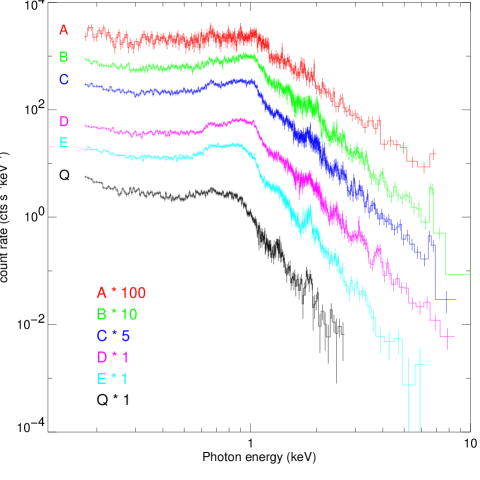
Figure 3: EPIC PN spectra during various stages of the flare (A–E) and during the pre-flare episode Q. The count rates have been multiplied by various factors to prevent mutual overlap (see factors indicated at lower left). Note the variable high-energy slope, indicative of variable flare temperatures.

The EPIC PN spectra shown in Fig. 3 characterize the spectral evolution of the large flare across episodes A – E (together with the low-level spectrum ’Q’). The individual spectra have been shifted along the y axis by factors indicated in the figure to avoid mutual overlap. The high-energy slope (between 1.5–7 keV) is largely determined by the bremsstrahlung continuum of the hottest dominant plasma component. As the flare progresses, the slope becomes steeper, indicative of overall cooling of the flare plasma. Also, a prominent Fe K complex including He-like Fe xxv lines is seen around 6.7 keV predominantly in the earlier flare phases and at flare peak. Again, these lines are indicative of the presence of very hot ($>10$ MK) plasma. And third, the Fe L-shell region around 0.6–1.0 keV is another characteristic indicator of temperature since it contains Fe lines with ionization stages between Fe xvii–Fe xxiv that shift the peak emission of the unresolved spectral maximum from $\approx 0.75$ keV in the pre-flare spectrum to $\approx$1 keV at flare peak, decreasing again as the flare progresses. Various line features above 1.4 keV can be used to constrain abundances of Mg, Si, S, Ar and Ca. We will present an abundance analysis below, combining EPIC information with RGS spectroscopy.

Reflection grating spectra obtained during the low-level episode before the flare and during four intervals from flare peak to late decay are shown in Fig. 4. (The spectrum obtained from interval A shows a very low signal-to-noise ratio; the analysis pertaining to this interval strongly relies on the EPIC PN spectrum.) A few important lines are marked. The spectra obtained during low-level emission (interval Q) and at flare peak (interval B) are strikingly different, indicating heating to high temperatures during the flare. For example, a marked enhancement of the continuum flux level is visible at flare peak, and the appearance of lines of Fe xx–Fe xxiv around 10–12 Å with peak formation temperatures between 10–20 MK indicate the presence of large amounts of hot plasma.

Figure 4: Fluxed RGS1+2 spectra referring to the intervals Q (pre-flare low level), and B–E (see Fig. 2 for reference). The bin resolution is 50 mÅ except for panel B where a resolution of 78 mÅ has been used to improve the signal-to-noise ratio.

The spectra were used to study emission measure (EM) distributions, abundances, densities, and optical depths at various stages of the flare development. We discuss results in the following subsections.

4.3 Spectroscopic density measurements

The He-like line triplets of O vii (at 21.6–22.1 Å) and of Ne ix (at 13.4–13.7 Å) can be used to obtain characteristic electron densities in the source region of the respective lines (Gabriel & Jordan 1969). The ratio of the fluxes of the forbidden line ($f$, $1s^{2}\leavevmode\nobreak\ {}^{1}S_{0}-1s2s\leavevmode\nobreak\ ^{3}S_{1}$, at 22.1 Å for O vii and at 13.7 Å for Ne ix) and the intercombination line ($i$, $1s^{2}\leavevmode\nobreak\ {}^{1}S_{0}-1s2p\leavevmode\nobreak\ ^{3}P_{1,2}$, at 21.8 Å for O vii and at 13.55 Å for Ne ix) are sensitive to the electron density $n_{e}$ in the range of $10^{9}-10^{12}$ cm^-3 for O vii and $10^{10}-10^{13}$ cm^-3 for Ne ix (Porquet et al. 2001). Further He-like triplets, in particular of Mg xi and Si xiii, are accessible within the RGS range, but the spectral resolution is insufficient to cleanly separate the the lines of the triplet, and the density-sensitive ranges ($>5\times 10^{11}$ cm^-3) are probably only marginally useful for typical coronal flare plasmas on dwarf stars.

In Paper I, we discussed the evolution of the $f/i$ ratios during the large flare episode; we will not repeat the analysis but briefly summarize the results. The densities derived from O vii flux ratios were found to peak around $4\times 10^{11}$ cm^-3 during the primary and secondary flare peaks (intervals B and D, respectively), while $n_{e}$ was lower by about one order of magnitude during the decay episodes (intervals C and E). These densities combined with the spectral measurement of the EMs of the O vii line forming plasma were used to estimate total masses and volumes during the flare. It was found that the mass of the relatively cool O vii forming plasma increased appreciably toward the decay episodes, possibly due to continuous cooling of plasma that was initially heated to much higher temperatures. The O vii line triplets are represented in flux units in Fig. 5 (B–E). Suppression of the $f$ line in panels B and D is clearly visible. The spectrum obtained during the low-level episode (Q) shows a line ratio compatible with fluxes around the lower limit of the density-sensitive range of the O vii triplet, corresponding to densities in the range $10^{9}-10^{10}$ cm^-3 (see Paper I).

Figure 5: O vii triplets during the low-level episode Q and during various flare intervals. The small number at upper right indicates the flux at the upper border of the plot. The three vertical lines mark the positions of the resonance, the intercombination, and the forbidden line (for increasing wavelength).

Figure 6: Same as Fig. 5, but for the Ne ix triplet. The dashed lines indicate two potentially strong, blending Fe xix lines.

The analysis of the Ne ix triplet (see Fig. 6 for an illustration of fluxed spectral extractions) is much more complicated due to strong blending with several lines in particular of Fe xix (Ness et al. 2003b, Fe xix has a peak formation temperature of about 8 MK, compared to 4 MK for Ne ix). While Fig. 6C and E do show a flux peak at the position of the $f$ line at 13.7 Å, its possible suppression in panels B and D cannot be established given the dominance of contributions from Fe xix at flare peak.

In principle, there may be some contributions to the $i$ and $f$ lines from the steady component; the $f/i$ ratios may thus be slightly biased by non-flare contributions. Since the $f$ line is much stronger than the $i$ line during the low-level emission (Fig. 5Q), the correction is essentially for the former flux. If the decaying trend of the overall light curve (Fig. 1) continues after the start of the large flare, then, for the intervals D–E, we expect an O vii flux about 2.5 times smaller than on average during the low-level interval Q, resulting in a non-flare $f$ flux about 13% of that observed during interval D. Correction of this effect would increase the density by about 15%, which is not significant given the considerable errors in the flux ratios. In any event, we note that the densities reported in Paper I are in this sense lower limits, but specific corrections are meaningless since we cannot accurately estimate the (small) contribution of the non-flare emission at any time during our strong flare. The effect of low-level contributions of course becomes more significant at later times during the flare decay. We have also investigated the $f/i$ behavior during the late secondary flare after $0.84$ d, but no significant density increase as in the earlier episodes could be observed.

It is interesting to note that the density behavior of this flare finds parallels in observations of large solar flares. McKenzie et al. (1980) presented O vii flux ratios during a large flare with similar time scales as ours and found $f/i$ ratios around unity close to the flare peak, implying densities of up to $2\times 10^{11}$ cm^-3. Much shorter flares were discussed by Doschek et al. (1981); in those cases, the densities reached peaks around $(10-20)\times 10^{11}$ cm^-3 as measured from O vii, but this occurred very early in these flares (during the flare rise), while during flare peak, electron densities of a few times $10^{11}$ cm^-3 were derived. As in our observations, the densities very rapidly decreased after the peak to levels at or below $10^{11}$ cm^-3. The estimated masses and volumes, on the other hand, steadily increased, a conclusion also drawn in Paper I for Proxima Centauri where we suggested that this indicates an increase of the amount of cool plasma that was initially heated to higher temperatures but that cools to a few MK. Unfortunately, we have no reliable density diagnostic for the more relevant flare temperatures. Doschek et al. (1981) and references therein report solar-flare densities derived from Fe xxv ($T>10$ MK) that are similar to those measured from O vii ($T\approx 2$ MK). Landi et al. (2003) recently used various density diagnostics for an M class solar limb flare. From Fe xxi lines, they derive densities up to $3\times 10^{12}$ cm^-3, but there are conflicting measurements for lower ionization stages that reveal much lower densities, comparable with pre-flare densities (see also references in that paper). If the density values at $\approx 10^{7}$ K are real, then pressure equilibrium cannot be assumed for flaring loops; a possible explanation involves volumes for the O vii and the Fe xxi/Fe xxv emitting plasmas that are spatially separate, possibly contained by different magnetic field lines. Obviously, further solar studies are needed.

4.4 Abundances and emission measure distributions

A derivation of elemental abundances is inherently related to the knowledge of the EM distribution because the formation efficiency of all observed X-ray emission lines in a collisionally ionized plasma is strongly dependent on the temperature structure. For previous efforts using high-resolution X-ray spectroscopy, see, e.g., Brinkman et al. (2001), Drake et al. (2001), Güdel et al. (2001a) and Audard et al. (2003a). EM distributions are also discussed in Huenemoerder et al. (2001). Despite some differences between the reported results, there is wide agreement that magnetically very active stars reveal an inverse First-Ionization Potential effect (Brinkman et al. 2001) that expresses itself in low abundances of elements with a low first ionization potential (FIP), and enhanced abundances of elements with a high FIP. This is in contrast to the Sun (von Steiger & Geiss 1989) and solar-like inactive stars in which a normal FIP effect has been found in similar X-ray studies (enhanced low-FIP elements; Güdel et al. 2002b).

There is particular interest in studying elemental abundances also during flares. Flares bring chromospheric and photospheric material into the corona after heating this cool gas and inducing chromospheric evaporation. Differences between the composition of flare plasma, chromospheric plasma, and the overall low-level coronal plasma could have important implications for mass transport or diffusion processes. While overall abundance changes in flares have been reported previously (e.g., Mewe et al. 1997), a selective FIP-related change of elemental abundances was first reported for a large flare on an RS CVn-type binary by Güdel et al. (1999). Similar enhancements of low-FIP elements during large flares on other RS CVn binaries were described by Osten et al. (2000) and Audard et al. (2001). We will test here whether similar enhancements are seen in the Proxima Centauri flare.

Despite the comparatively large count rates in the present flare on Proxima Centauri, the analysis of abundance anomalies and the differential EM distribution is challenging because of the short time scales of variability. We again use sections Q and A–E marked in Fig. 1 for the analysis. We subjected the PN and RGS1+2 data to the same analysis method as described in Audard et al. (2003a). In short, we used only the strongest emission lines of the RGS and their immediate surrounding wavelength ranges, in particular lines of Mg, Fe, Ne, O, N, and C, plus a few intervals of continuum. We thus preserve a correct treatment of the overlapping line wings in particular in the Fe L-shell region while discarding many regions containing weak and ill-defined emission lines with often poor atomic data. We also flagged wavelength intervals with poor instrumental calibration, in particular all data shortward of about 8.3 Å in the RGS. The description of the important hot flare plasma components requires additional information from the EPIC PN camera that sensitively constrains the hot end of the EM distribution by the bremsstrahlung continuum and the Fe K complex at 6.7 keV. Since the high-resolution RGS data discriminate much better between spectral features at lower energies, we used the PN data only above 1.3 keV (shortward of 9.3 Å). The combined PN + RGS1 + RGS2 data sets were then subject to a multi-component analysis in the SPEX software (Kaastra et al. 1996a) to derive an initial set of temperatures, EMs, and abundances. This procedure has the advantage of optimally considering all line blends and wings that may affect the selected line systems, while at the same time self-consistently calculating the (abundance and temperature-dependent) continuum level. The abundances were then used to derive a more comprehensive EM distribution. In principle, this procedure could be iterated, but the limited data quality at hand does not warrant a deeper analysis.

We report here the abundance ratios (with respect to the Fe abundance) and EM distributions obtained from the intervals Q and A-E. All ratios are normalized to solar photospheric ratios as given by Anders & Grevesse (1989). For Fe alone, we adopted an updated solar photospheric abundance reported by Grevesse & Sauval (1999). We prefer to use these traditional solar values for ease of comparison with previous X-ray studies. We do, however, also show the abundance ratios if the updated solar photospheric values of C and O presented by Allende Prieto et al. (2001, 2002) are used as a basis. The results relative to the former set of solar photospheric abundances are listed in Table 2 together with their 1$\sigma$ rms errors, and illustrated in Fig. 7 (filled circles). Since the updated Allende Prieto et al. photospheric abundances of C and O are smaller by factors of 1.48 and 1.74, respectively, than those given by Anders & Grevesse, the ratios in Fig. 7 increase by the respective factors. These modified abundance ratios are shown by open circles.

The most surprising aspect here is that the abundance ratios with respect to Fe are nearly constant across the range of FIP, and most ratios are actually close to solar photospheric values (ratios of unity). The abundances of Ne, N, and C tend to systematically exceed unity, although the effect is, given the error bars and unknown systematic errors in the atomic physics (in particular of several blending lines), rather small. If the updated solar abundances for C and O given by Allende Prieto et al. (2001, 2002) are considered, then there is some trend during the late flare phases for high-FIP elements to be higher than low-FIP elements (by factors of 2–3), while this trend is not visible during flare peak. We also quote the “absolute” abundance (with regard to H) of Fe for each interval; such values require good measurements of the continuum which we feel confident we have well determined using the high-energy tail of the EPIC PN spectrum (see Fig. 3), given the high dominant temperatures in the flare (Figs. 8, 9).

Figure 7: Elemental abundances determined during the low-level episode Q and during flare intervals A–E. All abundances are plotted as ratios to the Fe abundance, and are normalized with the respective solar photospheric abundance ratios according to Anders & Grevesse (1989). For Fe, an updated value given by Grevesse & Sauval (1999) has been used. The open circles refer to solar abundances of O and C reported by Allende Prieto et al. (2001) and Allende Prieto et al. (2002), respectively.

Fig. 8 and 9 illustrate two versions of the corresponding EM distributions. The former set was obtained by fitting Chebychev polynomials of order 6, while the latter set uses an integral inversion technique with a regularization parameter for the smoothness of the DEM (errors cannot be derived in the context of the polynomial fit, but comparing with the alternative regularization method illustrates the range of solutions). The differences between the methods are not surprising and relate to the ill-posedness of the underlying integral inversion problem. Details of these methods are described in Kaastra et al. (1996b). A comparative study of several inversion techniques is given in Güdel et al. (1997a). Overall, the polynomial method tends to reveal peaks in the EM distribution, while the regularization method shows extended wings up to high temperatures. The two versions illustrate the principal uncertainty in the reconstruction of an EM distribution but at the same time clearly illustrate the main thermal structure of the flare, and its change across the different flare phases. The lowest panel in each of these figures illustrates the evolution of the EM distribution by showing all DEMs on the same scale. Although the regularization method clearly spreads out the EM over a larger range than the polynomial method, the trends are the same: Rapid heating to high temperatures is followed by an increase of the EM to its peak at somewhat lower temperatures, after which the EM spreads out over a larger range while cooling.

Table 2: Abundance ratios with respect to Fe for various phases (A-E) of the large flare (values rounded to multiples of 0.1), and for the low-level pre-flare section (Q). All values are normalized with the solar ratios. The basic solar abundances of Anders & Grevesse (1989) have been used, except for Fe for which the value given in Grevesse & Sauval (1999) has been adopted. Errors are based on 1$\sigma$ errors of the individual abundances (see text for details). “Fe/Fe” is unity by definition, but the error bars indicate the fractional uncertainty of the Fe abundance. The last line gives the Fe abundance relative to solar photospheric values.

Element	Q	A	B	C	D	E
C/Fe	$1.9_{-0.7}^{+0.7}$	$1.8_{-1.9}^{+3.8}$	$0.7_{-0.3}^{+0.3}$	$1.6_{-0.4}^{+0.4}$	$1.7_{-0.4}^{+0.4}$	$2.0_{-0.4}^{+0.4}$
N/Fe	$1.5_{-0.6}^{+0.6}$	$1.7_{-1.9}^{+5.2}$	$1.1_{-0.4}^{+0.4}$	$1.2_{-0.4}^{+0.4}$	$1.5_{-0.4}^{+0.4}$	$1.9_{-0.4}^{+0.4}$
O/Fe	$0.6_{-0.2}^{+0.2}$	$1.1_{-0.7}^{+0.6}$	$0.5_{-0.1}^{+0.2}$	$1.0_{-0.2}^{+0.2}$	$1.1_{-0.2}^{+0.2}$	$1.2_{-0.2}^{+0.2}$
Ne/Fe	$1.6_{-0.6}^{+0.6}$	$2.4_{-2.1}^{+2.2}$	$1.3_{-0.3}^{+0.4}$	$1.8_{-0.4}^{+0.4}$	$1.6_{-0.3}^{+0.3}$	$2.3_{-0.4}^{+0.4}$
Mg/Fe	$2.1_{-0.8}^{+0.9}$	$0.2_{-0.2}^{+0.9}$	$0.6_{-0.2}^{+0.2}$	$1.2_{-0.3}^{+0.3}$	$1.6_{-0.3}^{+0.3}$	$1.3_{-0.3}^{+0.3}$
Si/Fe	$2.1_{-0.8}^{+0.8}$	$0.2_{-0.2}^{+0.4}$	$1.0_{-0.2}^{+0.2}$	$1.2_{-0.3}^{+0.2}$	$1.5_{-0.3}^{+0.2}$	$1.3_{-0.2}^{+0.2}$
S/Fe	$-$	$0.6_{-0.5}^{+0.6}$	$0.7_{-0.2}^{+0.2}$	$0.8_{-0.2}^{+0.2}$	$1.1_{-0.2}^{+0.2}$	$1.0_{-0.3}^{+0.3}$
Ar/Fe	$-$	$-$	$0.6_{-0.3}^{+0.3}$	$0.5_{-0.4}^{+0.5}$	$2.3_{-0.7}^{+0.7}$	$0.3_{-0.3}^{+0.9}$
Ca/Fe	$-$	$-$	$-$	$-$	$1.5_{-1.0}^{+1.0}$	$-$
Fe/Fe	$1.0_{-0.2}^{+0.3}$	$1.0_{-0.4}^{+0.4}$	$1.0_{-0.2}^{+0.2}$	$1.0_{-0.2}^{+0.2}$	$1.0_{-0.1}^{+0.1}$	$1.0_{-0.1}^{+0.1}$
Ni/Fe	$0.8_{-0.8}^{+0.9}$	$3.1_{-3.1}^{+3.0}$	$3.1_{-0.9}^{+0.9}$	$3.6_{-1.0}^{+1.1}$	$4.1_{-1.0}^{+1.0}$	$2.7_{-0.8}^{+0.8}$
Fe/H	$0.51_{-0.11}^{+0.16}$	$0.58_{-0.24}^{+0.26}$	$1.21_{-0.19}^{+0.20}$	$0.67_{-0.10}^{+0.11}$	$0.54_{-0.06}^{+0.07}$	$0.47_{-0.05}^{+0.06}$

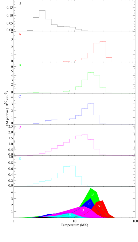
Figure 8: Emission measure distributions for the pre-flare interval Q and for flare intervals A–E, using a polynomial reconstruction algorithm that fits the DEM with polynomials of order 6. The lowest panel shows a superposition of all flare DEMs on the same absolute scale.

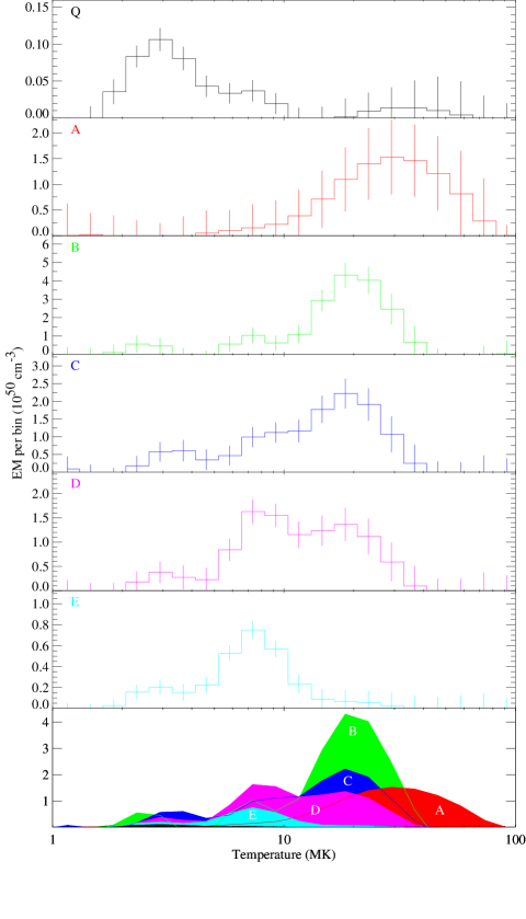
Figure 9: Similar to Fig. 8, but using a regularization inversion of the spectrum to obtain the EM distribution.

4.5 Optical depth

Standard interpretation of coronal emission assumes that the optical depth of the plasma is negligible for both line and continuum emission. Traditional spectral analysis of coronal EM distributions and elemental abundances would be fundamentally flawed if significant optical depths were present, and radiative transport methods would be in order. Schrijver et al. (1994) argued for non-zero optical depth due to resonant scattering in several lines of the inactive solar analog $\alpha$ Cen in the extreme ultraviolet range, a view that was challenged by a follow-up investigation including EM analysis from X-ray data (Schmitt et al. 1996). The situation is also rather unclear in the solar context. While Schmelz et al. (1997) and Saba et al. (1999) find evidence for optical depth effects in the Fe xvii $\lambda$15.01 line based on flux ratios with respect to the Fe xvii $\lambda$15.26 and the Fe xvii $\lambda$16.78 lines, recent laboratory measurements of these ratios significantly differ from previous theoretical calculations (Brown et al. 1998, 2001, Laming et al. 2000).

Stellar coronal optical depths have recently been studied using grating observations from XMM-Newton (Audard et al. 2003a) and Chandra (Ness et al. 2001, 2003a), with results compatible with negligible optical depths in stars across a wide range of activity levels. Conditions in large flares may, however, be different. Following Ness et al. (2003a), we measure line ratios between lines with low oscillator strengths, namely Fe xvii $\lambda$15.26 and Fe xvii $\lambda$16.78, and a line with a high oscillator strength, namely Fe xvii $\lambda$15.01. The flux in the latter is thus more likely to be reduced by resonant scattering. Experimentally, for zero optical depth $f(15.26)/f(15.01)=0.30-0.36$ (Ness et al. 2003a and references therein). For the $f(16.78)/f(15.01)$ ratio, previous theoretical values range between $0.40-0.50$, while newer calculations by Doron & Behar (2002) give a range between $0.60-0.75$ depending on temperature (see also the detailed description in Ness et al. 2003a and references therein).

The S/N ratio of our data was sufficient to derive some rough values for the above flux ratios. We fitted the lines with delta functions at their rest wavelengths convolved with the instrument response function. The continuum level was described, in the vicinity of the respective lines, by a power-law function. Since the line wings of the Fe xvii $\lambda$15.01 and the Fe xvii $\lambda$15.26 overlap and an intervening Fe xix line is also detected at $\lambda$15.20, these lines were simultaneously fitted. After a first iteration, the wavelengths of the brighter two lines (those at 15.01Å and 16.78Å) were optimized by using them as fitting parameters as well. The deviations were minor.

From our data, we find $f(15.26)/f(15.01)=0.18-0.31$ for the intervals C, D, and E where the S/N is sufficient for meaningful ratios, with an error of about $\pm(0.06-0.09)$ for each ratio. For $f(16.78)/f(15.01)$, we find, for the same three intervals, values of $0.43-0.62$, with errors of $\pm(0.06-0.12)$. We thus clearly do not detect any opacity effect at any of the flare phases investigated, at least within the large error ranges allowed by the present data. This suggests that even under extreme conditions of a flare plasma, optical depth effects are negligible, at least in the temperature range investigated with Fe xvii lines ($T\approx 3-8$ MK).

5 Interpretation and discussion

5.1 Small flares and coronal heating

The first portion of our observation shows continuous variability to an extent that no part of the observation can be defined as being “quiescent” for intervals exceeding $\approx 1$ hr (see Fig. 1), and often variability occurs on much shorter time scales. This is a new aspect made possible by XMM-Newton’s high sensitivity and the long uninterrupted monitoring (see also Audard et al. 2003b for a similar observation of the late-type M dwarf binary UV Cet). We suggest that the numerous small peaks visible in the X-ray light curve on time scales of 1–10 minutes are the most prominent examples of a large sequence of intermediately luminous flares, approximately corresponding to M class flares in the solar classification. Support for this view is manifold: i) The light curves of the small enhancements resemble typical flares on active stars or on the Sun (Paper I for examples). ii) We find many of these enhancements to be preceded by optical bursts similar to the standard behavior in solar flares, and also similar to the correlated light curves of the large Proxima Centauri flare. iii) Hardness increases during periods of enhanced low-level activity.

We suggested, in Paper I, that much of the X-ray emission observed during this observation may be due to the superposition of a large number of intermediate and weak flares, most of which cannot be individually resolved, therefore forming a pseudo-continuous emission level with sporadic enhancements due to the strongest but least numerous members of the distribution. The principal model we thus propose is fundamentally different from a static corona and is rooted in evidence that magnetically active stars show mean coronal properties that are at variance with a corona like the Sun’s. In a comparative study of solar analogs at different activity levels, Güdel et al. (1997b) studied stellar X-ray EM distributions as a function of total X-ray luminosity (or age) and compared them with time-averaged EM distributions of solar flares. They found that active stellar EM distributions resemble the superposition of a low-level solar EM distribution and a time-averaged EM of strong (solar) flares as interpreted from GOES satellite data. Toward lower-activity stars, the hot component becomes weaker, probably due to a smaller rate of flares heating the corona to high temperatures. The complete active-stellar EM distributions may thus be the result of stochastic, superimposed flaring (Güdel 1997) . In more active stars, the rate of strong flares is larger, but since larger flares heat more EM to higher temperatures than do small flares (Feldman et al. 1995), the time-averaged EM distribution develops a prominent high-temperature component additional to the low-T emission measure. The latter is, in this picture, due to the combined effect of microflares that heat the plasma to only a few MK. The physical cause for an increase of the flare rate, and hence for an increase of the rate of large flares heating a large amount of plasma to high temperatures, was suggested to be the increasing filling factor of active regions (Güdel et al. 1997b). As the concentration of active regions on an active star becomes larger, there are more interactions between tangled magnetic fields, leading to more numerous flares. The rate of very large flares thus also increases.

This interpretation is also in line with recent studies of longer time series obtained with the EUVE and BeppoSAX satellites (Audard et al. 2000, Kashyap et al. 2002, Güdel et al. 2003a; see also Butler et al. 1986) that suggest that all of the observed extreme ultraviolet and X-ray emission of active late-type main-sequence stars could be made up by a population of stochastic flares distributed in total energy as a power law, with the smallest flares dominating the energy budget. All observed X-ray emission characteristics would thus be a consequence of a multitude of superimposed flare rises and decays. For example, the EM distribution would be dominated by the statistical properties (temperature, density, volume) attained during the long flare decays (Güdel et al. 1997b, 2003a).

Proxima Centauri is, during its low-level episodes, a moderately active star only, with $L_{\rm X}/L_{\rm bol}\approx(0.6-2.4)\times 10^{-4}$, and with an EM distribution dominated by $\approx$3 MK plasma and a tail reaching to $\approx$10 MK (Figs. 8, 9). We expect large flares to be much hotter. Feldman et al. (1995) found a correlation between peak EM and peak temperature of solar and stellar flares. The faintest detectable flares in our observations were estimated to be $(2-5)\times 10^{26}$ erg s^-1 (Sect. 4.1), which implies EM $\approx(7-16)\times 10^{48}$ cm^-3 if a specific plasma emissivity per unit EM of $3\times 10^{-23}$ erg cm³s^-1 is taken as a basis (from the SPEX software for temperatures of a few MK, using solar abundances according to Table 2 for the flare peak; see Kaastra et al. 1996a). Fig. 2 in Feldman et al. (1995) then suggests flare peak temperatures of $15-20$ MK. Since these are only the largest of the contributing flares during low-level episodes and the characteristic temperatures during the long decay are typically a factor of two lower, our observations are well compatible with the view that low-level flares dominate the EM distribution.

Figure 10: Comparison of the fluxed RGS spectrum of YY Gem (bottom panel) with the spectrum obtained during the large flare (combined intervals A, B, C, and E; middle panel) on Proxima Centauri, and the low-level spectrum (Q; top panel). The spectral bin width is 43.74Å.

We can illuminate this problem from another angle. Extremely X-ray active M dwarfs with luminosities much higher than Proxima Centauri show higher characteristic coronal temperatures during low-level episodes. For example, the DEM of the active dM1e+dM1e binary YY Gem is dominated by plasma at $T=6-12$ MK (Güdel et al. 2001b). The light curve is, somewhat similar to Proxima Centauri, interspersed with intermediate and weak flares, while a quasi-steady emission level dominates the overall spectrum. The difference is that YY Gem’s low-level luminosity is two orders of magnitude higher. If the flare heating hypothesis as described above holds, then the low-level emission of YY Gem is dominated by proportionately larger flares, namely flares $\approx$100 times stronger than those barely seen during Proxima Centauri’s low-level emission, thus producing higher characteristic temperatures according to the Feldman et al. relation. Incidentally, the large flare on Proxima Centauri described here corresponds to such an event. We would then expect that the high-luminosity, long decay of the Proxima Centauri flare determines a spectrum that resembles the low-level emission of YY Gem. This is indeed the case. Fig. 10 compares the fluxed RGS spectra of the combined flare portions A, B, C, and E (omitting the secondary flare peak) with the integrated spectrum of YY Gem collected from a $\approx 1$ d observation (Güdel et al. 2001b). The spectral line ratios and the continuum level look surprisingly similar but differ significantly from the much cooler spectrum observed during Proxima Centauri’s low level emission. The flare DEM tends to be somewhat hotter than the integrated YY Gem DEM (Güdel et al. 2001b), and the Ne ix and Ne x lines at 13.45 Å and at 12.1 Å, respectively, tend to be somewhat lower in the Proxima Centauri flare compared to the Fe xvii lines, which is probably due to differences in the Ne/Fe abundance ratio (Fe xvii and Ne ix have very similar line formation temperatures). Note, however, that the DEM reconstruction presented by Güdel et al. (2001b) was based on RGS2 only; this spectrum is rather insensitive to temperatures significantly above 10 MK. The MOS spectra (Table 2 in Güdel et al. 2001b) indicate an additional large amount of EM around 20 MK (see also Stelzer et al. 2002). The presence of weaker flares and later flare decays will also increase somewhat cooler components in the DEM. This comparison again suggests that more active stars are dominated by flare-like plasma corresponding to intermediate-to-large flares, reaching to high temperatures, while lower-activity coronal emission may as well be composed of flare contributions which, given the lower flare energies, attain lower average temperatures. This hypothesis would explain i) why more active stars show hotter coronae, ii) why more active stars show much higher luminosities (due to the increased EM built up during the flare process). It further supports the model that active stellar coronae are heated by stochastic flares. And lastly, it may explain why active (main-sequence) stars show high characteristic densities. If low-level emission is made up of flares as the one discussed in this paper, then densities derived spectroscopically from the time-integrated spectrum across the entire flare should be similar to densities measured in active stars during quiescence. For the Proxima Centauri flare, we obtained an average characteristic density from the O vii triplet of log$n_{e}=10.50^{+0.32}_{-0.25}$, while, for example, the low-level YY Gem spectrum reveals a similar value, namely log$n_{e}=10.35^{+0.13}_{-0.45}$, as do many other active main-sequence stars (Güdel et al. 2001a, Ness et al. 2002).

5.2 Flare models

We will now discuss the large flare in the context of standard flare models. Various models have been discussed in the literature, although all of them represent simplified paradigms that may not be realized in the Sun or stars in their pure forms. Rather, we expect that some gross characteristics of the models may approximately describe the observations, thus providing some insight into the overall development of magnetic energy release. With this in mind, we will, in the following, describe two complementary models and investigate their applicability to large flares as the one presented here. The first approach, a 2-ribbon flare model based on work by Kopp & Poletto (1984) but extended to include approximate radiative and conductive cooling losses, was presented in this form by Güdel et al. (1999). The second approach, using full hydrodynamic simulations of a closed loop or a pair of loops, has been previously described by, e.g., Peres et al. (1982). We will discuss one typical numerical solution, but will defer an in-depth presentation of the hydrodynamic simulations to a companion paper (Reale et al. 2004). We begin this discussion by briefly reviewing some information on the initial energy release phase that can be extracted from the optical burst.

5.2.1 The impulsive phase of the flares

The initial energy release of a solar flare is in general most obviously seen at radio wavelengths, in the optical/UV regime, and in non-thermal hard X-rays. The relevant signals in these three wavelength regimes are thought to be related to high-energy electrons accelerated in the initial phase of a flare in the coronal reconnection region. While radio signals are due to gyrosynchrotron emission of electrons spiralling in the magnetic fields, the hard X-ray signal is due to bremsstrahlung when a non-thermal population of electrons impacts in the chromospheric/transition region layers at the magnetic field footpoints. At the same location, optical emission is thought to arise promptly due to heating and ionization of the chromospheric plasma. As this outline suggests, the three signatures of the impulsive flare phase should occur early in the flare, as the electrons are thought to be the cause for the subsequent chromospheric evaporation that then dominates the soft X-ray emission (Antonucci et al. 1984, Dennis 1988). For the optical emission observed in Proxima Centauri, this is clearly the case as was shown in Paper I (see also Fig. 2). Furthermore, solar observations clearly show - as expected - a very close time correlation between the hard X-rays and the microwave emission (Kosugi et al. 1988), and between optical “white light” and hard X-ray emission (Hudson et al. 1992; Dennis 1988 and references therein), often within seconds.

While solar research has made extensive use of non-thermal hard X-rays for the study of the energetics of the impulsive flare phase (Dennis 1988), the respective signals are presently out of reach for stellar astronomy since required detector sensitivities are not available at the energies of interest ($>$20 keV). However, observation of “white light” flares (or equivalently, as in this work) U band flares is relatively easy for M dwarfs given the large contrast of flares against photospheric background emission. The U band has traditionally played a major role since the flare enhancement is particularly large there. The physics of the continuum enhancement is not very well understood. Hudson et al. (1992) (and references therein) argue for excitation by energy transfer from electron beams, either by direct collisions, or by UV irradiation excited by the electron impact. For a further, short discussion on the issue, see Hawley et al. (1995).

Independent of the poorly understood physical cause of the U band emission, our observation, together with previous solar knowledge puts us into a position to at least grossly assess the time evolution of the primary energy release in electrons if the standard model outlined above holds. The U-band light curve (above its photospheric level) would thus be a sensitive tracer of the production of non-thermal particles in the corona, and therefore an efficient proxy of the inaccessible non-thermal hard X-ray emission so often seen in solar flares.

A second application is possible, namely to roughly determine the chromospheric footpoint area of the flaring magnetic fields, as outlined in Hawley et al. (1995). To do this, one would have to know the temperature of the U-band emitting source, requiring at least one more observation in another optical band, which is not available. The analysis by Hawley et al. (1995) for flares on the M dwarf AD Leo suggests temperatures of $\approx 9000-9500$ K under the assumption of blackbody emission. Assume that the filling factor of the flare footpoints in the projection onto the sky is $X$. Since the area emitting at the non-flaring photospheric temperature is reduced by the flaring area, the U-band luminosity ratio between measurements taken during the flare and outside the flare is

$$R={L_{f}+(1-X)L_{q}\over L_{q}}={XB_{\rm U}(T_{f})+(1-X)B_{\rm U}(T_{q})\over B_{\rm U}(T_{q})}.$$ (1)

Here, $L_{f}$ is the U-band flare luminosity, and $L_{q}$ is the U band quiescent luminosity of the whole star; $B_{\rm U}$ is the Planck function evaluated in the U band ($\approx 3500$Å) for the flare temperature ($T_{f}=9000$ K, see above) and for the photospheric effective temperature outside flares ($T_{q}$ = 2700 K, Frogel et al. 1972), respectively. Therefore, recalling that $B_{\rm U}(T)\propto(\mathrm{exp}(hc/k\lambda T)-1)^{-1}\approx\mathrm{exp}(-41156/T)$, we find

$$R=1+X\left(e^{41156(1/T_{q}-1/T_{f})}-1\right)\approx 1+4.3\times 10^{4}X.$$ (2)

Our flare increased the U band flux by a factor of $R\approx 20$, so that the fractional projected area of the footpoints is $\approx 4\times 10^{-4}$ of the cross section of the star. If this described one circular footpoint, then its diameter would be 2% of the stellar diameter. Comparing with the results we will derive from X-rays below, the area covered by U-band emitting footpoints must be considerably smaller than the X-ray emitting area, which is compatible with magnetic loops that span over a wide range across the stellar surface.

5.2.2 A two-ribbon flare model

The two-ribbon (2-R) flare model devised initially by Kopp & Poletto (1984) is intrinsically a parameterized magnetic-energy release model in which the time development of the flare light curve is fully determined by the amount of energy available in non-potential magnetic fields, and the rate of energy release as a function of time and geometry. The complete time evolution of the flare is based on continuous heating that feeds an evolving reservoir of hot plasma. Plasma cooling is not included in the original model; it is assumed that a portion of the total energy is radiated into the observed X-ray band, while the remaining energy will be lost by other mechanisms. 2-R flares are well established for the Sun; they often lead to large, long duration flares that may be accompanied by mass ejections. This configuration is clearly suggestive for our observation, paralleling conclusions for similar flares observed previously on Proxima Centauri (Haisch et al. 1983). We will describe here an extension of the model that includes approximations of radiative and conductive losses, and that will also take into account some geometric development of the radiating magnetic structures. This variant of the 2-R model was first applied to a large, long-duration flare observed on the RS CVn-type binary UX Ari (Güdel et al. 1999). A detailed description is given in the latter reference; we give a brief summary below.

A 2-R flare conceptually starts when a disruptive event, e.g., a filament eruption, opens a loop arcade. The open field lines are then driven toward a radial neutral sheet (above the magnetic neutral line) where they reconnect at progressively higher altitudes, forming a system of overlying loops below them. The excess energy provided by annihilation of the magnetic fields is released in an unspecified form. The amount of continuous heating provided throughout the reconnection episode principally describes both the flare increase and its decay.

The magnetic fields are, for convenience, described along meridional planes on the star by Legendre polynomials $P_{n}$ of order $n$, up to the height of the neutral point; above this level, the $B$ field is directed radially. The magnetic fields are thus assumed to be poloidal, initially directed radially outward and then reconnecting, starting with the antiparallel field lines closest to the neutral line. As time proceeds, field lines further away from the neutral line move inward at coronal levels and reconnect at progressively larger heights above the neutral line. The reconnection point thus moves upward as the flare proceeds, leaving closed magnetic loop systems underneath. One loop arcade thus corresponds to one (N-S aligned) lobe between two zeros of $P_{n}$ in latitude, axisymmetrically continued over some longitude in E–W direction. The propagation of the neutral point in height, $y(t)$, with a time constant $t_{0}$ (in units of $R_{*}$, measured from the star’s center) is prescribed by

$$y(t)=1+{H_{\rm m}\over R_{*}}\left(1-e^{-t/t_{0}}\right)$$ (3)

$$H(t)\equiv[y(t)-1]R_{*}$$ (4)

and the total energy release of the reconnecting arcade per radian in longitude is equal to the magnetic energy lost by reconnection,

$${{\rm d}E\over{\rm d}y}={1\over 8\pi}2n(n+1)(2n+1)^{2}R_{*}^{3}B^{2}I_{12}(n){y^{2n}(y^{2n+1}-1)\over[n+(n+1)y^{2n+1}]^{3}}$$ (5)

$${{\rm d}E\over{\rm d}t}={{\rm d}E\over{\rm d}y}{{\rm d}y\over{\rm d}t}$$ (6)

(Poletto et al. 1988). In Eq. (3), $H_{\rm m}$ is the maximum height of the neutral point for $t\rightarrow\infty$; typically, $H_{\rm m}$ is assumed to be equal to the latitudinal extent of the loops, i.e.,

$$H_{\rm m}\approx{\pi\over n+1/2}R_{*}$$ (7)

for $n>2$ and $H_{\rm m}=(\pi/2)R_{*}$ for $n=2$. Here, $B$ is the surface magnetic field strength at the axis of symmetry, and $R_{*}$ is the stellar radius. Finally, $I_{12}(n)$ corresponds to $\int[P_{n}({\rm cos}\theta)]^{2}d({\rm cos}\theta)$ evaluated between the latitudinal borders of the lobe (zeros of ${\rm d}P_{n}/{\rm d}\theta$), and $\theta$ is the co-latitude. We have evaluated this expression for lobes that are centered at the star’s equator for odd $n$, and lobes that start at the equator for even $n$. Note that $R_{*}$, $B^{2}$, and $I_{12}(n)$ merely define the normalization of the energy release light curve, not its form. The latter is determined by the time constant $t_{0}$ and the polynomial order $n$.

The largest realistic two-ribbon flare model is based on the Legendre polynomial of degree $n=2$; the loop arcade then stretches out between the equator and the stellar poles. For simplicity, we assume that the arcade extends along a great circle on the stellar surface, e.g., the equator (instead of adopting axisymmetric arcades at any other stellar latitude), although the computations of the latitudinal and radial geometry use the exact equations as given by Kopp & Poletto (1984). Since solar two-ribbon flares occur in loop arcades whose length is typically about 1.5 times their width (Poletto et al. 1988), we adopt this ratio for any given $n$: $L=1.5H_{\rm m}=3R_{*}\pi/(2n+1)$.

The Kopp & Poletto model is applicable after the initial flare trigger mechanism has terminated, although Pneuman (1982) suggested that reconnection may start in the earliest phase of loop structure development. The time of strong production of non-thermal electrons, signified by the optical burst during the X-ray increase, gives rise to explosive chromospheric evaporation and steeply increasing temperatures. This phase of the flare may be less well described by the model.

Poletto et al. (1988) introduce an ad hoc factor of 10% of the magnetically released radiative energy that escapes into the X-ray regime. Here, we include time-dependent conductive and radiative losses in the X-ray corona self-consistently and hence account for the emitting volume. The volume and the observed EM provide an overall electron density for which we obtained estimates from the He-like line triplets in the RGS spectra. Requiring that the densities agree with the measured densities will thus constrain the model parameters, in particular $n$. The radiative loss time is

$$\tau_{\rm r}={3kT\over n_{\rm e}\psi}$$ (8)

where $\psi$ is the emissivity per unit EM of the hot, optically thin plasma, which we take to be $\psi=2.5\times 10^{-23}$ ergs s^-1cm³ for $T=15-20$ MK (from the collisional ionization equilibrium model in the SPEX software, see Kaastra et al. 1996a). The downward conductive flux in a constant cross section loop is

$$F_{\rm c}=-\kappa T^{5/2}{\partial T\over\partial s}$$ (9)

with $s$ being the length parameter along the loop, and $\kappa\approx 10^{-6}$ ergs cm^-1s^-1K^-7/2 (Spitzer 1962). $F_{\rm c}$ can be approximated as

$$F_{\rm c}\approx-\eta\kappa{T_{\rm m}^{7/2}\over l},$$ (10)

where the peak temperature $T_{\rm m}\approx T$, $\eta=4/7$ has been introduced by Kopp & Poletto (1993) to account for the geometry in this approximation, and $l$ is the time-dependent semi-length of the loop,

$$l(t)\approx{\pi\over 2}H(t).$$ (11)

Cooling is principally controlled by radiation and conduction with time constants of $\tau_{\rm r}$ and $\tau_{c}$, respectively, leading to an effective cooling time $\tau_{\rm e}$ given by

$${1\over\tau_{\rm e}}={1\over\tau_{\rm c}}+{1\over\tau_{\rm r}}.$$ (12)

Combining the relevant equations (see Güdel et al. 1999 for details) one obtains for the model X-ray luminosity

$$L_{\rm X}(t)=f(t){{\rm d}E\over{\rm d}t}{L\over R_{*}}$$ (13)

and the underlying EM must be

$${\rm EM}(t)=f(t){{\rm d}E/{\rm d}t\over\psi(T)}{L\over R_{*}}.$$ (14)

Here, $f(t)=\tau_{\rm e}(t)/\tau_{\rm r}(t)$ gives the fraction of the total energy being emitted as X-rays, and $L/R_{*}$ denotes the length of the arcade in radians, here taken to be $\leq 2$ ($L=1.5H_{\rm m}$). We adopt $T$ from the observations, $T\approx 20$ MK during the period of consideration. Note that the observable X-ray emission is not proportional to ${\rm d}E/{\rm d}t$ in Eq. (13) as the fraction $f$ is time dependent. The run of the electron density $n_{\rm e}$ then is

$$n_{\rm e}(t)={{\rm d}E/{\rm d}y\over 3kTR_{*}\pi H(t)}.$$ (15)

The electron density is solely determined by the geometry of the arcade, as prescribed by Eq. (3)–(7).

We integrated all relevant equations in short time steps for a given $n$, adjusting $t_{0}$ and $B$ until a good fit to the observations was obtained. Following Güdel et al. (1999), we assume that only a fraction $q<1$ of the liberated magnetic energy is used to heat the plasma (energy that is lost via radiation and conduction, while the remaining fraction is transformed into mechanical energy, into fast particles ejected from the corona, etc). Kopp & Poletto (1984) use $q=0.003$ in their application to a solar flare.

As the overlying magnetic field lines reconnect, the loops already reconnected are pushed downward until they asymptotically reach a final position, corresponding to a potential field configuration. We have assumed that the X-ray loops have relaxed to this final geometry while radiating most of their X-ray energy (corresponding to $t\rightarrow\infty$). The derivation of the asymptotic loop configuration is performed by piecewise integration as described in Güdel et al. (1999).

There are only few independent parameters for this model. The total energy released is controlled by $B^{2}$, and by the efficiency $q$. To obtain the same thermal energy, $q$ obviously scales as $q\propto B^{-2}$. The fraction of radiated X-ray energy out of the total thermal energy is given by $f(t)$. These factors together thus determine the X-ray flare amplitude. The time scale is given by the parameter $t_{0}$ in Eq. (3). Additionally, Eq. (15) provides an approximation of the loop density that can be compared with the observations. There is thus a family of solutions $(B,q)$ for each $n$. The best-fit solution for $n=2$ is shown in Fig. 11 (top) and required a maximum surface magnetic field strength of $B=2050$ G for $q=0.01$. A larger efficiency of $q=0.05$ thus corresponds to $B=920$ G. These two examples characterize the probable range for $B$ although stronger fields have also been measured in late-type dwarfs (Johns-Krull & Valenti 2000). The time constant $t_{0}\approx 4000$ s, and the final height of the neutral point (for $t\rightarrow\infty$) is $H_{\rm m}\approx 1.73\times 10^{10}$ cm or 1.7$R_{*}$ for $n=2$.

For $n=3$, we find $B=2720$ G for $q=0.01$, and $t_{0}=3300$ s. Similarly, for $n=4$, the best-fit parameters are, for $q=0.02$: $B=2200$ G and $t_{0}$ = 3100 s. Since we can also estimate the model densities from Eq. (15), our observations of density-sensitive spectral lines, in particular O vii, provide a further constraint. For $n=2$, Fig. 11 shows an electron density at flare peak of $n_{\rm e}\approx 3\times 10^{11}$ cm^-3, quite compatible with the O vii measurements. The latter refer to much cooler plasma than the bulk plasma in a flaring loop at its peak luminosity. However, as discussed in Sect. 4.3, densities inferred for hot solar flare plasma seem to be of similar magnitude as densities derived from the O vii lines. For $n=3$, densities at flare peak are $\approx 5\times 10^{11}$ cm^-3, while for $n=4$, $n_{e}\approx 7\times 10^{11}$ cm^-3. In the latter case, the magnetic field estimated from the model at the loop top and at the time of flare peak is below the pressure equilibrium value if the electron temperature is $\approx 20$ MK. We therefore tend to exclude solutions for $n=4$ and higher within the context of this simple model.

The model fits well until about $t=1000$ s after flare start; thereafter, the model light curve clearly decays too fast, which is due to the emergence of the secondary flare. Indeed, at $t\approx 1000$ s, the hardness ceases to decay and develops a plateau (see Fig. 2), presumably due to resumed heating (Reale et al. 2004). We emphasize that in the framework of this model, the flare density is not a consequence of cooling material condensing out of the corona and falling back to the surface. Rather, the loops radiating at later times are less dense than those radiating at earlier times, according to Eq. (15). The 2-R model does not describe the evolution of plasma within a loop, but rather the plasma and geometry parameters of a series of loops in time.

    

Figure 11: Top: Simulation of the large Proxima Centauri flare using a simple 2-R flare model described in the text. The best fit shown here is for $n=2$, $B=2050$, $t_{0}=4000$, $q=0.01$. The solid line shows the model X-ray luminosity, to be compared with the observations that are plotted by small crosses. The dotted curve indicates the electron density (see scale on the right), and the two solid lines at the bottom of the figure mark the height of the emitting loop (see scale on the right). The model clearly decays too fast beyond $t=1000$ s after flare start, which is due to the emergence of a secondary flare. - Bottom: Similar to upper figure, but here the light curve synthesized from a time-dependent hydrodynamic simulation of plasma confined in a single footpoint-heated loop is overplotted (solid line). The heating lasts 600 s. The flare start is defined slightly differently to optimize the fit to the rise phase (the precise start of the flare cannot be defined from the soft X-rays unambiguously). Further details are described in Reale et al. (2004).

We have to check the value of the decay time $\tau_{\rm e}$. The model presented here assumes that the decay time $\tau_{\rm e}$ is short compared with the evolution of the flare. If this were not the case, then a significant portion of the energy released at earlier times would contribute to the emission at time $t$, i.e., the light curve would be a convolution with radiation from previous times. From Fig. 2, we estimate that changes in the light curve occur on a time scale of about 1000 s near flare peak. The fit is satisfactory if $\tau_{\rm e,r}\la 1000$ s up to the flare peak. Our evaluation of Eqn. (12) indicates that $\tau_{\rm e}=80-100$ s around the flare peak for the acceptable solution presented in Fig. 11, and the radiative loss time $\tau_{\rm r}$ is around 800–1000 s, which is compatible with our requirements.

We caution that the assumptions for this flare model are crude. The purpose of our estimates, however, is to indicate whether the observed flare belongs to a class of compact flares or may be a global phenomenon, compatible with the standard two-ribbon flare model. Our results thus suggest that the flare is likely to be geometrically large, with size scales (height, footpoint separation) on the order of $10^{10}$ cm or one stellar radius. The presence of such extended coronal structures is compatible with VLBI observations that show flaring cores that rapidly evolve into extended structures (Mutel et al. 1985). Observed radio sources reveal size scales on the order of the stellar diameters (Benz et al. 1998). Also, the absence of radio eclipses or strong signatures of rotational modulation in long-duration flares on similar M dwarfs agrees well with the assumption of extended flare geometries on such stars (Alef et al. 1997).

5.2.3 Hydrodynamic flaring loop model

X-ray flares can alternatively be modeled using full numerical hydrodynamic simulations. We outline the method here, but for a technical description, we refer to Peres et al. (1982) and Reale et al. (2004). The latter reference discusses applications to the present observation in deeper detail. The numerical approach stresses on plasma confinement. The basic assumption becomes that the flare is mostly governed by the evolution of the plasma confined in a magnetic loop and that changes of the loop system geometry and size are small, slow and play a minor role.

One can then focus on modeling the flaring plasma confined in a single unchanging loop, where it moves and and transports energy along the magnetic field lines. The magnetic field does not play any role directly, except for plasma confinement.

The confined plasma behaves as a compressible fluid and its evolution can be described with a one-dimensional time-dependent hydrodynamic model. When solving the equations of conservation of mass, momentum and energy, in coronal plasma conditions, several physical terms are important, and, in particular, the pressure gradients, the stellar gravity, the radiative losses and the thermal conduction. Describing all of them requires the numerical solution of the hydrodynamic equations. A parameterized and time-dependent heating function is included to trigger the flare. A sufficiently intense heat pulse is able to make the plasma temperature increase to flare values and to drive a strong plasma evaporation from the chromosphere: the combination of these two effects switches the flare on. The flare decay is instead mostly driven by the plasma cooling by radiation and thermal conduction, after the heating pulse has finished, unless a residual heating is able to sustain the decay. This makes an important conceptual difference from standard 2-R models, in which the decay is assumed to be totally driven by the release of magnetic energy during the reconnection of progressively larger arches.

Several numerical time-dependent loop models have been applied to study solar coronal flares. One of them has been applied to study part of a flare observed on Proxima Centauri with the Einstein satellite (Reale et al. 1988).

In an accompanying paper we model the flare for most of its duration, including the second peak, by describing the evolution of flaring plasma confined in single loop structures. The detailed numerical approach allows us to synthesize the plasma X-ray emission at the focal plane of the EPIC PN and to make detailed comparisons with the real data. We present the overall results of a simulation here for comparison with our analytic approach using the 2-R formulation.

In the simulations, the flaring plasma confined in a single loop is able to explain well the rise phase, main peak and initial decay of the flare (Fig. 11, bottom), and the addition of an arcade of similar flaring loops allows to explain the second peak and the late decay. In spite of the different approach, the results are not in contrast to those obtained with the 2-R modeling described in Sect. 5.2.2. Hydrodynamic modeling and detailed comparison of results to data will however allow us to obtain specific constraints on the loop geometry and on the heating function throughout the flare, and insight in the physical flaring plasma conditions. In particular, the loop height appropriate for the simulations is very similar to the typical height found in the 2-R model, namely $\approx 0.6\times 10^{10}$ cm. This result is thus in good agreement with estimates based on the 2-R model. The principal finding from the modeling is thus that the flaring source is intrinsically large, of order of one stellar radius.

6 Conclusions

Proxima Centauri is the closest star to the Sun, and it belongs to the important class of magnetically active stars as well. The latter are generally characterized by enhanced spot coverage indicating a large surface magnetic filling factor, chromospheric emission lines such as H$\alpha$, enhanced flaring activity, or strong coronal emissions. Proxima Centauri does not show signatures of extreme activity but given its surface area of about 2% the Sun’s, its X-ray luminosity equaling an average solar level is notable. A more important aspect of the present and all previous X-ray investigations of this star is in fact simply its very late spectral type, which has two important implications : First, since optical flare emission is predominantly “blue”, a large contrast against the weak, red photospheric emission makes optical flare detection easy. Our OM data have been an important guide to recognize low-level flaring in the X-ray light curve. And second, there is quite limited surface area to host active regions of a size that would be typical for the Sun. In fact, Proxima Centauri is no larger than a large solar coronal active region (Reale et al. 2004). This circumstance makes X-ray observations very sensitive to reconfigurations in the corona that likely affect a considerable portion of the surface. This obviously helped set a good contrast for the large number of weak flares we have detected during the low-level X-ray emission.

Our observation has captured a continuously variable X-ray corona, with flares spanning two orders of magnitude in peak flux and at least three orders of magnitude in total X-ray energy. The weakest flares seen during the low-level episode are principally the weakest of their kind observed on any active star, while the large flare is the largest yet seen on Proxima Centauri, exceeding even some of the strongest solar X-ray flares. Despite this large range of flare parameters, we find similar timing characteristics among them: Many X-ray flares are preceded by optical bursts, suggesting the process of chromospheric evaporation by electron bombardment as the main driver of heating and mass transport into the corona. The large flare is only set apart by its very slow decay and secondary peaks that indicate continued heating.

We interpret the low-level emission as being predominantly due to a superposition of stochastic flaring. While a truly quiescent emission level due to steadily heated coronal loops cannot be excluded, the continuous decay of emission by a factor of ten during the first 12 hours of our observation requires relatively rapid reconfiguration of the corona unless the complete flux decay is due to the late decay of a large flare that reached its peak before our observation started. (Rotational modulation of active regions is not likely to be important on the observed time scales; the rotation period of Proxima Centauri is suspected to be as long as 83.5 d, see Benedict et al. 1998.) The additional modulation on time scales of hours and associated hardness changes argue for physical changes in the corona on such time scales. If most of the low-level emission originates from flaring plasma, then the flare peaks individually detected constitute the strongest examples of a population of low-level flares. As such, they determine the high-temperature cutoff of the emission measure distribution since flare peak temperatures are dependent on the peak emission measure (Feldman et al. 1995). We have argued that the expected temperatures for these flares are roughly commensurate with the observed EM distribution: the DEM shows a high-T extension to $\approx 15$ MK, which is the expected peak temperature for the largest flare during the low-level emission.

If this picture has some merit, then it should apply to other stars at higher activity levels. For a characteristic distribution of flare energies as seen on the Sun, higher flare rates also induce larger rates of larger flares. Therefore, a larger flare rate (above a certain threshold energy) brings more material into the corona and at the same time heats some of it to much higher temperatures according to the Feldman et al. relation. We thus expect characteristic temperatures in more active stars to be higher, which is generally the case. We have scaled this model to the extremely active dMe binary YY Gem, which shows an X-ray luminosity $\approx$100-200 times higher than Proxima Centauri. The largest flares frequently dominating the low-level emission of YY Gem are consequently similar in energy to the large flare in Proxima Centauri that we captured during the second half of our observation. The combined spectrum of the latter flare indeed resembles the average spectrum of YY Gem, and so do the EM distributions although a full modeling should take into account the additional lower-energy flares occurring on YY Gem as well.

We therefore suggest that the low-level emission of magnetically active stars is made up, to a large fraction, by a superposition of flares over a large range of total energies. The flare rate (above a given low-energy threshold) determines the high-temperature end of the EM distribution of the intervals perceived as “low-level”. A natural consequence of this model is that, as the flare rate increases toward more active stars, the emission measure increases because more chromospheric evaporation is taking place, while the large amount of EM produced by larger flares is also heated to higher temperatures, thus inducing a hotter EM distribution in these stars. We thus suggest that the Feldman et al. (1995) relation naturally explains why stars at a higher activity level show hotter coronae.

The large flare observed during the second part of our observations has offered a number of new views on extremely large stellar flares. Like most of the other, low-level flares, the earliest phase of the rapidly heating X-ray episode is accompanied by a very large optical burst. From solar analogy, we interpret this “white light” flare as being the signature of accelerated electrons bombarding the chromosphere and evaporating the material that is subsequently becoming visible in X-rays. In this sense, we find that U band flares are ideal and sensitive proxies for the non-thermal hard X-rays ($>20$ keV) often investigated in solar flare research.

While the emission mechanism of the optical flare is somewhat uncertain, we infer relatively small areas for the chromospheric footpoints. This is in contrast to the X-ray geometry we find from two different approaches (an analytic 2-R model and a fully hydrodynamic approach). Both X-ray flare models indicate relatively large flares, with typical size scales of $10^{10}$ cm or one stellar radius. While Proxima Centauri is much smaller than the Sun, the size of such active regions is comparable to those that produce very large flares on the Sun.

For the first time, X-ray spectroscopic measurements have fully resolved the electron density development during a stellar flare, indicating peak densities in the $1-5$ MK plasma of approximately $4\times 10^{11}$ cm^-3. Such values are similar to densities measured during solar flares. We have also measured the abundance development during several stages of the flare. Apart from a trend toward higher abundances of high-FIP elements, the abundance ratios are relatively close to solar photospheric ratios.