Modeling an X-ray Flare on Proxima Centauri: evidence of two flaring loop components and of two heating mechanisms at work

We model in detail a flare observed on Proxima Centauri with the EPIC-PN on board XMM-Newton at high statistics and high time resolution and coverage. Time-dependent hydrodynamic loop modeling is used to describe the rise and peak of the light curve, and a large fraction of the decay, including its change of slope and a secondary maximum, over a duration of more than 2 hours. The light curve, the emission measure and the temperature derived from the data allow us to constrain the loop morphology and the heating function and to show that this flare can be described with two components: a major one triggered by an intense heat pulse injected in a single flaring loop with half-length $\approx 1.0\times 10^{10}$ cm, the other one by less intense heat pulses released after about 1/2 hour since the first one in related loop systems, probably arcades, with the same half-length. The heat functions of the two loop systems appear be very similar: an intense pulse located at the loop footpoints followed by a low gradual decay distributed in corona. The latter result and the similarity to at least one solar event (the Bastille Day flare in 2000) indicate that this pattern may be common to solar and stellar flares, in wide generality.

1 Introduction

Coronal flares are known to be very complex phenomena, and to involve multiple coronal structures, multiple spectral bands and multiple physical mechanisms at a time. Furthermore, it is very difficult to define a typical coronal flare pattern (e.g. Golub & Pasachoff 1997). A “standard” classification, of solar coronal flares divides them into two main categories, based fundamentally on the topology of the involved structures: compact flares and long-enduring events (Pallavicini et al. 1977). Compact flares occur mostly inside single loops whose shape and volume do not change significantly during the flare. Long-enduring events, instead, occur in loop arcades, and higher and higher loops are typically involved as the flare progresses. The arcade footpoints, best seen in the H$\alpha$ line, appear as two ribbons getting more distant with time. Long-enduring events are generally more gradual and longer-lasting than compact flares, but exceptions exist.

The soft X-ray light curve of flares consists, generally, of a steep rising phase, a well-defined peak and a slower – generally exponential – decay. A gradual rise or a decay composed by segments with different e-folding times (e.g. Osten & Brown 1999) can also occur.

Stellar flares are spatially unresolved and we have no direct information on the morphology of the coronal structures involved, except in the presence of eclipses during the flare (Schmitt & Favata 1999). The similarity of solar and stellar X-ray flares, however, suggests that also stellar flares involve plasma confined in closed structures.

Empirical methods have been developed to infer the size of the flaring structures from the e-folding decay time of light curves (Kopp & Poletto 1984, White et al. 1986, Poletto et al. 1988, van den Oord & Mewe 1989, Pallavicini et al. 1990, Hawley et al. 1995, Reale et al. 1997, Reale & Micela 1998, see Reale 2002 for an extensive review of these methods). In the hypothesis of flares occurring inside closed coronal structures, the decay time of the X-ray emission roughly scales as the plasma cooling time. In turn, the cooling time scales with the length of the structure which confines the plasma: the longer the decay, the larger is the structure (e.g. Haisch 1983). A loop thermodynamic decay time has been derived (van den Oord & Mewe 1989, Serio et al. 1991) as:

$$\tau_{th}=\frac{120L_{9}}{\sqrt{T_{7}}}$$ (1)

where $L_{9}$ and $T_{7}$ are the loop half-length and the maximum temperature of the flaring plasma, in units of $10^{9}$ cm and $10^{7}$ K, respectively. The timescale above is derived under the hypothesis of impulsive heat released at the beginning of the flare. However, a significant heat released during the decay may increase the decay time, and therefore lead to overestimate the loop length, if not correctly diagnosed (Reale et al. 1997, Reale 2002). By means of extensive hydrodynamic simulations of decaying flaring loops, Reale et al. (1997) derived an empirical formula for the loop length, combining the information from the light curve and the trajectory of the flare in the density-temperature diagram :

$$L_{9}=\frac{\tau_{LC}\sqrt{T_{7}}}{120f(\zeta)}\leavevmode\nobreak\ \leavevmode\nobreak\ \leavevmode\nobreak\ \leavevmode\nobreak\ \leavevmode\nobreak\ \leavevmode\nobreak\ \leavevmode\nobreak\ \leavevmode\nobreak\ f(\zeta)\geq 1$$ (2)

where $\tau_{LC}$ is the decay time derived from the light curve. This formula can be obtained from the expression of the loop thermodynamic cooling time (Eq.1), but includes a non-dimensional correction factor $f(\zeta)$, larger than one (i.e. a shorter loop length) if significant heating is present during the decay. The slope $\zeta$ of the decay path in the density-temperature diagram (Sylwester et al. 1993) is maximum ($\sim 2$) if the heating is negligible in the decay and minimum ($\sim 0.5$) – the slope of the loci of the hydrostatic loops with decreasing temperature – if the heating dominates the decay. This approach has been tested on a sample of solar flares observed with Yohkoh/SXT (Reale et al. 1997) and extensively applied to flares observed on stars of various spectral type (Reale & Micela 1998, Favata et al. 2000, 2001, Maggio et al. 2000, Güdel et al. 2001).

The empirical methods are of easy application and appropriate to infer the size of the flaring loops and some information on the flare heating, provided that the light curve and the temperature and emission measure diagnostics are available with enough photon statistics and time resolution and coverage to derive a decay trend.

An XMM-Newton observation of the nearest star Proxima Centauri, of spectral type dMe, includes a very well-observed flare, already presented in Güdel et al. (2002, hereafter Paper I) and further analyzed in Güdel et al. (2003, hereafter Paper II). Other flares have been observed on Proxima Centauri and studied in detail (Haisch et al. 1983, Reale et al. 1988, Poletto et al. 1988, Byrne & McKay 1989). However, the large effective area and the high time coverage of XMM-Newton has allowed to collect data at an unprecedented level of detail which motivate a deeper analysis aimed at a higher level of diagnostics.

Time-dependent hydrodynamic loop models have been shown to provide a good description of the evolution of the flaring plasma (e.g. Peres et al. 1987, Reale & Peres 1995, Hori et al. 1997). In particular, in the hypothesis of compact flares, it is customary to assume that plasma moves and transports energy only along the magnetic field lines, and to consider one-dimensional models (e.g. Nagai 1980, Peres et al. 1982, Doschek et al. 1983, Nagai & Emslie 1984, Fisher et al. 1985, MacNeice 1986, Gan et al. 1991).

The light curve of the flare observed with XMM-Newton shows a very peaked maximum and a globally slow decay, with changing e-folding time and even a well-defined smoother secondary peak. In this work, the flare is modelled in detail throughout the late phases, well after the second peak. The high quality of the data and their detailed comparison to the model results allow us not only to constrain the length of the main flaring loop, but also to diagnose the involvement of other structures in the flare, and to constrain the heating functions (intensity, temporal and spatial distribution) of all the flaring structures.

In Sect. 2 we describe the observation and the constraints on the modeling, in Sect. 3 we describe our modeling approach in detail; in Sect. 4, the simulations performed and the results obtained are presented, in Sect. 5 the results are discussed and in Sect. 6 conclusions are drawn.

2 The observation

The flare has been detected during the observation of Proxima Centauri made by XMM-Newton (Jansen et al. 2001) on 2001 August 12, with a total exposure time of 65 ks. Fig. 1 shows the flare light curve in the 0.15 - 10 keV band, collected, in small window mode, with the PN detector (Strüder et al. 2001) of the European Photon Imaging Camera (EPIC, Turner et al. 2001); MOS detectors are affected by pileup problems. High resolution X-ray spectra between 0.35 and 2.5 keV, taken simultaneously with the Reflection Grating Spectrometers (den Herder et al. 2001), are also available, and in particular OVII 22 Å and Ne IX 13.5 Å He-like lines have been detected during the flare and analyzed in detail, yielding density estimates (Paper I). All data were analyzed using the XMM-Newton Science Analysis System (version 5.3, for RGS data version 5.4.1). The flare covers most of the final 20 ks of the observation with a maximum luminosity $L_{X,0.15-10}\approx 3.9\times 10^{28}$ erg/s. A large optical burst was captured with the Optical Monitor (Mason et al. 2001) in the rise phase of the X-ray flare, and may be a tracer of the production of non-thermal particles in the corona (Paper II).

Figure 1: Upper panel: Light curve (10 ks) of the flare on Proxima Centauri on 12 August 2001 as detected with the XMM-Newton EPIC-PN detector in the 0.15-10 keV band. The flare can be segmented into six phases, two rising (R1, R2) and four decay ones (D1-D4), bounded by the vertical dashed lines. The solid lines mark the decay trends. Time t=0 corresponds to 17:00 UT of 12 August 2001. Lower panel: hardness ratio (ratio of 1-4.5 keV to 0.4-1 keV count rates) in the same time interval as the light curve. Time resolution is 300 s.

Fig. 1 shows the light curve of the first 10 ks of the flare, and the hardness ratio (ratio of 1-4.5 keV to 0.4-1 keV count rates) in the same time interval (see also Paper II). The count rate in the figure is the raw one extracted from the selected image region which includes 90% of the total counts and should be further multiplied by the dead-time correction factor of 1.41. The bin size is 20 s. The corresponding PN spectra, collected in 16 time intervals as shown in Fig. 2 have been fitted with 2-T MEKAL models (Mewe et al. 1995) in XSPEC (Arnaud 1996). Fig. 2 shows the values obtained for the dominant hotter component throughout the flare.

The count rate reaches values as high as $\sim 122$ cts/s (after corrections). We can identify different phases of the light curve, which will be relevant for the modeling. During the initial rising phase (hereafter R1), the emission increases steeply by about two orders of magnitudes reaching a maximum in $\sim 1$ ks. The following decay is initially relatively rapid (D1, with a duration of $\approx 0.5$ ks) and then becomes slower (D2, $\approx 1$ ks). The time of the switch from D1 to D2 coincides with the time when the hardness ratio stalls and changes to a constant level (Fig. 1). After $\approx 2.5$ ks since the beginning of the flare, the light curve rises again (R2), slowly, for $\approx 1.7$ ks, reaching a second smoother peak at $\sim 40$ cts/s. The following decay is similar to the one after the first peak: fast first (D3, $\approx 1$ ks) and then slower (D4, $\approx 5$ ks). The light curve in phases D1, D2, D3 and D4 can be reasonably approximated with exponentials, with e-folding times $\tau_{D1}=1.45\pm 0.08$ ks, $\tau_{D2}=2.66\pm 0.12$ ks $\tau_{D3}=1.62\pm 0.06$ ks and $\tau_{D4}=4.35\pm 0.06$ ks, respectively, shown in Fig. 1.

Figure 2: Temperature and emission measure diagrams during the flare: the upper panel shows the density-temperature (n-T) diagram of the dominating component of the 2-T fitting, where EM^1/2 has been used as proxy for the density. The dashed line marks the evolution of the values and the end point of each phase is labelled. The lower panels show the evolution of the temperature and emission measure separately. Dashed lines as in Fig. 1.

Fig. 2 shows that the maximum fit temperature of the hot component, $\log(T_{obs})\approx 7.4$, is reached in phase R1, somewhat earlier than the maximum of its emission measure $\log(EM)\approx 51.3$.

In the hypothesis that the bulk of the flare, the first peak, occurs inside a single flaring loop, the e-folding time of the light curve and the slope of the n-T path in the initial decay can be used to estimate the loop half-length, according to Eq. (2), calibrated for the XMM-Newton EPIC/PN spectral response, already applied to a few events (Güdel et al. 2001, Stelzer et al. 2002, Briggs & Pye 2003), with:

$$F(\zeta)={c_{a}}\exp(-\zeta/\zeta_{a})+q_{a}$$ (3)

where

$$c_{a}=11.6\pm 0.5\leavevmode\nobreak\ \leavevmode\nobreak\ \leavevmode\nobreak\ \leavevmode\nobreak\ \leavevmode\nobreak\ \zeta_{a}=0.56\pm 0.06\leavevmode\nobreak\ \leavevmode\nobreak\ \leavevmode\nobreak\ \leavevmode\nobreak\ \leavevmode\nobreak\ q_{a}=1.2\pm 0.1$$

$$\leavevmode\nobreak\ \leavevmode\nobreak\ \leavevmode\nobreak\ \leavevmode\nobreak\ \leavevmode\nobreak\ \leavevmode\nobreak\ \leavevmode\nobreak\ \leavevmode\nobreak\ \leavevmode\nobreak\ \leavevmode\nobreak\ \leavevmode\nobreak\ \leavevmode\nobreak\ \leavevmode\nobreak\ \leavevmode\nobreak\ \leavevmode\nobreak\ \leavevmode\nobreak\ \leavevmode\nobreak\ \leavevmode\nobreak\ \leavevmode\nobreak\ \leavevmode\nobreak\ \leavevmode\nobreak\ \leavevmode\nobreak\ \leavevmode\nobreak\ \leavevmode\nobreak\ \leavevmode\nobreak\ \leavevmode\nobreak\ \leavevmode\nobreak\ \leavevmode\nobreak\ \leavevmode\nobreak\ 0.4<\zeta\leq 1.9$$

An expression for the loop maximum temperature $T_{7}=T_{max}/(10^{7}$ K) can be derived from fitting hydrostatic model loops with isothermal models:

$$T_{max}=0.184\leavevmode\nobreak\ T_{obs}^{1.130}$$ (4)

We obtain $\log(T_{max})\approx 7.6$.

From Fig. 2, it can be noted that the initial decay D1 is very short and only two points are defined in the n-T diagram, too few to obtain a well-defined decay trend. If one assumes the initial decay D1 is entirely due to plasma cooling, with negligible heating, the empirical expression of loop length (Eqs. (2), (3) and (4)) yields an upper limit to the loop half length $L_{up}\approx 1.6\times 10^{10}$ cm.

The emission measure shows a second peak during phase R2, as the light curve does, while the temperature is practically flat. Phase D3 includes just two points with large error bars. Phase D4 is better defined: the temperature and EM of the hot component both decay monotonically, the temperature more slowly.

3 The modeling

3.1 The set up

The general approach to model this flare is an evolved version of the modeling of another flare observed on Proxima Centauri in 1980 with the Einstein Imaging Proportional Counter (Reale et al. 1988). At variance with the previous modeling effort, here the modeling will include later phases of the flare and more than one loop component, allowing us to diagnose contributions of flaring structures other than the main loop and the heating function at late times.

The model assumptions are those typical of a solar coronal flare loop modeling (e.g. Reale 2002): the flare in each loop is triggered by a strong heat pulse; the loop is initially at equilibrium (Serio et al. 1981) at the temperature ($\sim\leavevmode\nobreak\ 4$ MK) of an active region loop, not far from the peak of the EM distribution in quiescent conditions ($\approx\leavevmode\nobreak\ 3$ MK in Paper II). The flaring plasma is described as a fluid confined in a closed semicircular loop with fixed geometry and constant cross-section, perpendicular to the stellar surface and unchanged during the flare. The plasma moves and transports energy only along the magnetic field lines running parallel to the loop, and can therefore be described with a single curvilinear coordinate. The plasma evolution is then described by the time-dependent hydrodynamic equations of mass, momentum and energy conservation as done in many previous works (see references in Section 1), including, as significant physical effects, the gravity, the compressional viscosity, the radiative losses from optically thin plasma, and the thermal conduction. The stellar gravity and radius have been assumed $g_{*}=10g_{\sun}$ and $R_{*}=0.15R_{\sun}$, respectively (Pettersen 1980, Ségrensan et al. 2003). There are two external energy inputs: a low, constant and uniform one, which keeps the loop initially at equilibrium; a high and highly transient one, $Q(s,t)$, which triggers the flare, and is assumed to be a separable function of space $g(s)$ and time $f(t)$ (e.g. Peres et al. 1987):

$$Q(s,t)=H_{0}\leavevmode\nobreak\ f(t)\leavevmode\nobreak\ g(s)$$ (5)

where $H_{0}$ is the peak value of the heating rate, $s$ is the coordinate along the loop, $t$ is the time. We consider Gaussian spatial distributions, centered on $s_{0}$ and with width $\sigma$:

$$g(s)=\exp\left[-\frac{(s-s_{0})^{2}}{2\sigma^{2}}\right]$$ (6)

There is no reliable way to determine a priori the intensity, the spatial distribution, the duration and the time dependence of the heating function. We therefore proceed by educated guesses and refine the choices with the feedback coming from the comparison of the data to the model results. We will consider, in particular, three alternative distributions $g(s)$: two thin Gaussians centered at the footpoints, a single wide Gaussian centered at the apex, and a uniform heating ($\sigma\gg L$). As for the time dependence, we will consider a heat pulse, described as $f(t)=1$ for $0<t\leq\delta t_{H}$, and $f(t)=0$ at any other time. The heating decay is assumed exponential:

$$f(t)=\exp[-(t-t_{d})/\tau_{H}]$$ (7)

The time-dependent hydrodynamic equations have been solved using the revised version of the Palermo-Harvard numerical code with adaptive regridding (Betta et al. 1997, Betta et al. 2001). Symmetry with respect to the apex has been assumed, and a half-loop modelled.

A flaring loop model is set up by selecting the loop length and the heating function. The details and conditions of the loop before heat ignition are not critical for the simulation results, provided that the pressure is high enough to have a significant amount of mass in the chromosphere for evaporation (see Sect. 4).

3.2 The analysis of the results

The numerical solutions of the 1-D hydrodynamic plasma equations are in the form of plasma density, temperature and velocity distributions along the loop at progressing times. For comparison with observational data, from each density and temperature distribution, the plasma X-ray spectrum at the focal plane of the EPIC-PN detector is synthesized as done in several previous works (e.g. Reale et al. 1988, Reale et al. 1997, Reale & Micela 1998). We consider the MEKAL spectral code (Mewe et al. 1995) with a metallicity Z=0.5, as on average found in the spectral fits (Paper II). The MEKAL spectra are folded with the EPIC-PN response function used in Güdel et al. (2001). The final results are weakly dependent on the details (or minor changes) of the response function, since they are mainly based on the analysis of global observables, such as the light curve in a broad spectral band (0.15 - 10 keV). The normalization of the light curve obtained from the loop model to the observed one provides the loop cross-section area, which is a free parameter in the model.

The loop model spectra are fitted with single temperature (1-T) model spectra (the same as those used to synthesize them). The fitting provides a best-fit “average” temperature $T_{fit}$, and an analytical normalization factor, which, multiplied by the loop cross-section area, yields the emission measure. The 1-T fitting is performed in the 0.8-10 keV sub-band. This allows us to compare $T_{fit}$ to the temperature of the hot component of the multi-temperature fitting of the data, at least for $T_{fit}\ga 10$ MK.

Whenever fitting the observation data requires the combination of two model loops, we synthesize the total emission at a given time by summing the two focal plane spectra – one for each loop, with the appropriate cross-section area – at that time. We then analyze the resulting sequence of spectra, one for each time, as we do for single loop spectra: we derive the light curve and fit the spectra with single temperature models.

4 The results

The modeling of this flare will be described following the flare evolution. It will first address the flare peak, i.e. phases R1 and D1 in Fig. 1, then the first decay (D2), and finally the second peak and the late decay (R2, D3 and D4).

4.1 The flare peak

We model the initial and most intense phase of the flare with a single flaring loop; we will call it loop A.

4.1.1 The length of loop A

The modeling requires, first of all, that we set the loop length. As mentioned in Section 2, the empirical scaling laws applied to phase D1 provide an upper limit $L_{max}=1.6\times 10^{10}$ cm. In the lack of a well-defined path in the n-T diagram, and therefore of reliable information about the heating decay, any length shorter than this may be appropriate.

We will show here results for three loop half-lengths, namely the upper limit $L=1.6\times 10^{10}$ cm, an intermediate value $L=1.0\times 10^{10}$ cm and the half-length obtained for the Einstein flare ($0.7\times 10^{10}$ cm, Reale et al. 1988). The initial base pressures are $p_{0}=3$ dyne cm^-2 for the first two, and $p_{0}=4.3$ dyne cm^-2 for the last length value.

4.1.2 The heat pulse

The flare peak is driven by a strong heat pulse. The time dependence of the heat pulse is described in Section 3.1. The data indicate a very rapid increase of the temperature and therefore an impulsive heating. Typically in flares (and in their simulations as well) the emission measure still increases well after the heating has been turned off (e.g. Svestka 1976). The temperature is a better tracer of the heating duration, because the efficient thermal conduction makes it promptly decrease as the heating decreases. Fig. 2 and the time evolution of the hardness ratio (Fig. 1) suggest a duration of the order of 500 s; the choice of a pulse duration $\delta t_{H}=600$ s is good for all our simulations of this flare phase.

A hint for the pulse intensity comes from the flare maximum temperature. It is reached after a few seconds and then remains steady as long as the heating is constant, because thermal conduction rapidly balances the heating. By applying the loop scaling laws (Rosner et al. 1978) with $\log T=7.6$ (Section 2), we obtain that, if the heating were distributed uniformly in a loop of half-length $10^{10}$ cm, its intensity would be of the order of:

$$E_{H}\approx 10^{-6}T^{3.5}L^{-2}\approx 4\leavevmode\nobreak\ \rm erg\leavevmode\nobreak\ cm^{-3}\leavevmode\nobreak\ s^{-1}$$ (8)

For this phase of the flare, we have considered two alternative spatial distributions of the heat pulse along the loop: i) just above the footpoints ($s_{0}=0.1L$ and $\sigma=0.03L$); ii) centered at the apex ($s_{0}=L$ and $\sigma=0.3L$). The width of the heating distribution influences the simulation results little.

4.1.3 Modeling phases R1 and D1

Figure 3: Left: Fitting the observed light curve (data points) of the phases R1 and D1 with hydrodynamic simulations of a single flaring loop. The figure shows the light curves obtained from a loop with half-length $10^{10}$ cm heated at the footpoints (solid line) and at the apex (dotted line), from a loop with half-length $0.7\times 10^{10}$ cm heated at the footpoints (dashed line), and from a loop with half-length $1.6\times 10^{10}$ cm heated at the apex (dashed-dotted line). Right: corresponding paths in the EM^1/2-T diagram, obtained from fitting the model and the observed spectra with isothermal models (only the first five data points are shown).

We will not report on the whole exploration of the space of the model parameters that we performed, but only on some cases providing representative results. We will discuss results for the three loop lengths listed in Section 4.1.1. For the intermediate loop length ($L=10^{10}$ cm), we show results for two cases, i.e. a heat pulse concentrated at the loop footpoints with a maximum intensity of $H_{0}=60$ erg cm^-3 s^-1, and a heating deposited at the loop apex with a maximum intensity $H_{0}=12$ erg cm^-3 s^-1. For the smallest length, we show results for a heat pulse concentrated at the loop footpoints with a maximum intensity of $H_{0}=85$ erg cm^-3 s^-1. For the longest loop, we show results for a heat pulse at the loop apex with a maximum intensity of $H_{0}=10$ erg cm^-3 s^-1.

The evolution of the flaring plasma confined in a loop is well-known from extensive previous modeling studies (e.g. Peres et al. 1982). The global characteristics of the evolution do not depend on the details of the heating (see also Section 5.5): the heat pulse makes the temperature increase up to several tens MK along the whole loop in a few seconds, due to the high plasma thermal conduction; the dense chromosphere at the loop footpoints is heated violently, and expands upwards with a strong evaporation front. The upcoming plasma fills up the loop, very dynamically first and then more gradually, approaching a new hydrostatic equilibrium at a much higher pressure. The loop X-ray emission increases mostly following the increase of emission measure. As the heating stops (or decreases), the temperature promptly begins to decrease everywhere in the loop. As mentioned in Sect. 4.1.2, the emission measure peaks later and then decreases too, with the timescale of the plasma cooling. The different modeling choices lead to different time scales, values of density and temperature, and to different details of the evolution, which, in turn, determine differences in the X-ray emission and its evolution.

Fig. 3 shows the light curves obtained from computing 3000 s of plasma evolution for the four representative models described above (two for the intermediate loop, one for the short loop and one for the long loop). The model results are sampled with a minimum sampling time of 20 s. The model light curves are matched to the data by synchronizing the light curve maxima. The loop cross-section areas obtained from the normalization of the light curves are 3.6, 4.2, 1.1 and 4.0 $\times 10^{18}$ cm², corresponding to aspect ratios $R/L=0.11,0.12,0.08$ and 0.07, respectively, where $R$ is the radius of the loop cross-section, assumed circular.

The light curves all rise steeply during chromospheric evaporation, and the steepness decreases when the evaporation becomes more gradual. The maximum occurs about 400 s after the heat pulse has stopped, and the decay follows the decrease of the emission measure due to plasma cooling.

The rising phase obtained from modeling the shorter loop is too slow to fit reasonably well the observed one. The emission evolution obtained with the long loop is too gradual around the flare maximum, due to the longer time scales implied, and is not able to describe the sharp flare peak.

The light curves obtained with the intermediate loop fit better both the rising and the peak phase. The heating at the footpoints fits the maximum better than the heating at the apex. The rise is slower with the shorter loop because the initial evaporation front takes less time to fill the loop, and, since then, the density – and the X-ray emission – increases more gradually.

The T vs EM^1/2 plot of Fig. 3 shows the paths obtained from fitting the spectra of the four flare models, at various times, to isothermal model spectra, in comparison with fittings of the data (first five points). All models match reasonably well the first four data points, all included in phase R1 and D1. They depart from the fifth data point, which belongs to a later phase, as the light curves do after time $t\sim 1500$ s, and exactly where the hardness ratio stops decaying and gets constant (Fig. 1).

The results shown so far suggest us that the model which best fits phases R1 and D1 of the flare is the one with the loop of intermediate length ($L=1.0\times 10^{10}$ cm) and the heating at the footpoints. We will consider this as the starting point for fitting the following phases.

4.2 The decay phase D2

In phase D2, the decay of the light curve slows down significantly, as shown in Fig. 1. This trend cannot be explained with the cooling of a longer loop (Eq. (1)), because the decay is initially faster. Nor can it be explained with a heating gradually decaying from the peak value: there would be a single slower decay trend.

This change of slope may be explained in two alternative ways: i) in loop A, a low residual heating, much lower than the initial impulsive heating and with a different evolution, remains active; ii) another loop is beginning to flare and its rising emission overlaps the emission of loop A, slowing down the overall decay, and determining also the second flare peak (R2$+$D2).

The latter hypothesis will be discussed in the next paragraph, together with later flare phases. We now explore the hypothesis of the residual heating: it must be significantly less intense than the strong initial pulse, so as to become important only later in the decay, and must decrease gradually so to drive the late decay. We neglect the effect of such residual heating as long as the initial pulse is on.

Figure 4: Fitting the observed light curve (data points) of the flare phase D2 with a decaying heating switched on at the end of the heating pulse at the footpoints: uniform in corona and initial intensity 1.2 erg cm^-3 s^-1 (solid line), the same with initial intensity 0.75 erg cm^-3 s^-1 (dotted line), and with a decaying heating deposited at the footpoints (15 erg cm^-3 s^-1, dashed line). Data points as in Fig. 3.

Fig. 4 shows the fitting obtained with three different decaying heating functions, each switched on at the end of the heating pulse deposited at the footpoints, i.e. $t_{d}=600$ s and $\tau_{H}=4500$ s in Eq. (7): a) uniform in corona, and with intensity $H_{0}=1.2$ erg cm^-3 s^-1; b) the same, with lower intensity $H_{0}=0.75$ erg cm^-3 s^-1; c) at the footpoints, with the same spatial parameters as the impulsive heating and with intensity $H_{0}=15$ erg cm^-3 s^-1. Integrating over the loop length, the total rates of the heating a) and c) are $\approx 1/4$ of the total rate of the impulsive heating, heating b) $\approx 1/6$. The loop cross-section area obtained to best-fit the light curve down to phase D2 slightly changes to 3.3, 3.5, and $3.2\times 10^{18}$ cm², respectively.

It is immediately apparent that the residual heating deposited at the footpoints cannot describe the light curve in phase D2. At time $t\approx 2500$ s a thermal instability occurs, and the light curve first increases and then suddenly drops: indeed any decaying heating deposited at the footpoints has been found to be unable to describe this decay phase, because a thermal instability invariably occurs.

Phase D2 appears instead to be described more adequately with the residual heating deposited uniformly in corona and as low as 1/4 of the impulsive heating rate at t = 600 s. An even lower heating rate makes the emission decrease too fast. An equal amount of heating more localized anywhere in the coronal part of the loop (e.g. at the apex) does not bring significantly different results, and we will henceforth refer to a residual heating generically deposited in the corona.

4.3 The second peak and late decay: phase R2, D3 and D4

After time $t\approx 2500$ s, the light curve rises again to form the second lower maximum. The question, of course, is how this maximum is produced. Occam’s razor argument would suggest us simply that a second heating pulse, weaker than the first one, occurs in loop A around that time. However, we find that a second heat pulse as intense as to produce the necessary emission increase in the same loop invariably leads to a temporary temperature increase; such temperature increase is not observed (Fig. 2). On the contrary, the temperature stays constant in phase D2 and slightly decreases in phase R2. A similar trend is present also in the time evolution of the hardness ratio (Fig. 1).

The only way to produce the second emission peak with no significant temperature change is that a second loop system gets involved in the flare, and its emission adds to the one of loop A. We call this second loop, loop B, and model it separately from loop A. In addition to its length and its heating function, for modeling loop B we have to set a time shift of the heating switch on with respect to loop A. It is not trivial to constrain all these parameters because the evolution of loop B must be decoupled from the decay tail of loop A.

Figure 5: Fitting the observed flare light curve (data points) from phase R1 to D3 with a model consisting of the sum (solid line of a footpoint-heated flaring loop with half-length $10^{10}$ cm (with no decaying heating, dotted line)), and of a second top-heated flaring loop with half-length $2.5\times 10^{10}$ cm, ignited at the same time as loop A (dashed line). The two lower panels show the emission measure and temperature versus time obtained from fitting the model and the observed spectra with isothermal models. Data points as in Figs. 1 and 2.

We start noticing that phases D3 and D4 of the light curve (Fig. 1) are similar to phases D1 and D2: the decay is initially faster and then slows down. The e-folding time in phase D3 is only slightly longer than the one in the corresponding D1 phase (see Sect. 2 and Fig. 1). We take this as an indication that loop B may be similar to loop A, i.e. same length, and we choose to check this assumption against the possibility of a much longer loop B, namely L=2.5 $\times 10^{10}$ cm. Indeed, loop B could be even shorter than loop A, if a residual heating were present during phase D1. However, this would imply two different regimes of residual heating, one in phase D1 and another in phase D2, and introduce another set of free parameters in the modeling, which we prefer not to do, if unnecessary.

Since the slower evolution expected from a longer loop may naturally lead to a delayed emission peak, we have explored the possibility that the flare in this long loop B is triggered at the same time as that in loop A, with a lower intensity and longer duration. In this hypothesis, the slower decay D2 may be explained with the superposition of the continuation of the fast decay D1 with the rise of the flare of loop B (hypothesis (ii) in Sec. 4.2). In this specific scenario, we will drop the decaying heating in loop A.

Fig.5 shows the results obtained with a heating pulse located at the top of loop B with $H_{0}=1$ erg cm^-3 s^-1, constant for 3200 s. The figure shows the light curve of the two flare components separately, and the light curve obtained by summing the spectra of loop A and loop B (with distinct cross-section areas) at corresponding times, compared to the observed light curve. The light curve of loop B rises very gradually and peaks at time $t\approx 3500$ s, more than 2000 s later than the flare in loop A. The loop cross-section of this second loop that best fits the light curve is $6.2\times 10^{18}$ cm², which corresponds to quite a small aspect ratio $R/L\approx 0.06$. Fitting the total spectra of loop A$+$loop B with isothermal models, the global evolution of the emission measure is well described. The evolution of the temperature instead shows a deep minimum at time $t\approx 2000$ s. This is not present in the data, and suggests us to reject this model. A similar temperature dip appears also if such long loop B is heated at the footpoints.

Figure 6: Fitting the observed flare light curve (data points) from phase R1 to D3 with a model consisting of the sum (solid line) of two flaring loop systems with the same half-length and similar heating function: one (loop A, dotted line) is heated 2600 s earlier and 10 times more intensely than the other (loop B, dashed line). A residual heating sustains the decay of both loops. Data points and lower panels as in Fig. 5.

Fig. 6 shows results obtained with a loop B twin of loop A, and with a heating duration and spatial distribution of loop B identical to that of loop A, but triggered 2600 s later, with a rate ten times lower, $H_{0}=6$ erg cm^-3 s^-1. In this alternative scenario, the decaying heating of loop A is maintained. The best-fitting cross-section area of loop B is $16.7\times 10^{18}$ cm², five times larger than the area of the first flaring loop, or, equivalently, an arcade of five loops equal to loop A. This combination describes better the temperature trend, but the light curve shows a small dip at time $t\sim 3000$ s. As suggested by the residuals, the dip can be filled – and the fit further improved – simply by adding a third minor flaring component, adjusting the loop cross-section areas and the heating time shifts appropriately (Fig. 7). The best combination that we find is to add two loops B with area $9.0\times 10^{18}$ cm² and $10.8\times 10^{18}$ cm² (2.5 and 3 times the area of loop A, still compatible with an arcade of $\sim 5$ loops equal to loop A), and heated with time shifts of 2200 s and 2800 s, respectively, since the start of the heating of loop A.

Figure 7: Fitting the observed light curve (data points) of the whole flare including two other flaring loop components. Residuals (data counts minus model counts) are also shown. Data points as in Fig. 3.

In alternative, we may think to fill the gap of the light curve by considering a longer-lasting heating pulse in loop B, but we checked that this choice fails to reproduce adequately the temperature evolution.

The latest decay D4 can be reasonably well fitted by assuming a residual heating of loop B (or of two loops B) with the same characteristics and e-folding time as the one of loop A, and the superposition of the decays of loops A and B.

5 Discussion

5.1 The general scenario

This work describes the hydrodynamic loop modeling of an X-ray flare observed on Proxima Centauri with XMM-Newton. The data are very detailed: we can distinguish six well-defined phases in the light curve and a well-defined path in the density-temperature diagram. Our approach has been to model each phase in detail taking the time-resolved density/temperature information into account.

We find that this flare is best-described with the following combination of components:

• The initial phase of the flare, including the rise phase, the main peak and the initial decay, occurs in a single loop, loop A, with half-length $1.0\times 10^{10}$ cm.

• This phase is triggered by a heat pulse deposited at the loop footpoints over $\sim 10$ min.

• A (four-fold) weaker residual heating is left in loop A. It is deposited in the coronal section of the loop and decays slowly with an e-folding time of $\sim 1$ hour.

• About half an hour after the first heat pulse has stopped, other minor heating pulses ignite other loops, probably an adjacent arcade, and produce a second minor peak in the light curve.

• The loop arcade is made of $\sim 5$ loops with same length and cross-section area as loop A.

• The heating function of the arcade is very similar to that of the main flare.

Table 1 summarizes the parameters of the model flaring loops.

Table 1: Parameters of best-fit loop models

Parameters	Loop A	Loop B
Geometry
Half-length ($10^{10}$ cm)	1.0	1.0
Cross-section ($10^{18}$ cm2)	3.3 (3.6)a	17 (20)b
Aspect (R/L)	0.10 (0.11)a	0.22 (0.25)b
Morphology	Single loop	Arcade ($\sim 5$ loops)
Heat pulse
Location	footpoints	footpoints
Ratec ($10^{28}$) erg/s	27	14
Start time (s)	0	2600 (2200 - 2800)b
Duration (s)	600	600
Total energyc ($10^{32}$ erg)	1.6	0.8
Heat decay
Location	corona	corona
Initial ratec ($10^{28}$) erg/s	7.2	1.8
Start time (s)	600	3200 (2800 - 3400)b
$e$-folding time (s)	4500	4500
Total energyc ($10^{32}$ erg)	3.2	0.8
Plasma parameters
Max. temperature (MK)	46	20
Max. apex density ($10^{11}$ cm-3)	1.1	0.2
Max. velocity (km/s)	1400	800

^a - If no residual heating is included in the decay phase.

^b - assuming that two arcades of loops B are ignited in a sequence (600 s one from the other).

^c - assuming a loop aspect 0.10 and 0.22, respectively.

Hydrodynamic modeling allowed us to derive a very detailed scenario with qualitative and quantitative constraints on the loop morphology and on the heating function. The modeling may not be unique: we cannot exclude that other combinations of the parameters may be found with a significantly higher modeling effort, and a few parameters are not totally constrained.

On the other hand, we notice that such a complex and detailed event is reasonably well-described in terms of only two dominant loop components and a well-defined heating function, valid for both flaring loops. This result may provide a general pattern for the interpretation of stellar flares, even those which show light curves more complex than a simple rise$+$decay.

The complex light curve of this flare may be in part explained by the larger collecting area of XMM together with its capability of long uninterrupted observations with respect to previous satellites, and we may have missed it in other stellar flares just because of insufficient S/N ratio and time coverage. On the other hand, there are stellar flares observed with enough time resolution, coverage and statistics, which are less complex (e.g. van den Oord & Mewe 1989, Pallavicini et al. 1990), and also many solar ones (e.g. Sato et al. 2003).

If the data quality were not so high, we would not have been able to distinguish so many details of the light curve and to address them one by one, and we would have limited our analysis, for instance, to an overall application of the empirical scaling law (Eq. (2), (3), (4)) approximating the decay to a single decay. We would have obtained a decay time $\tau_{sin}\sim 4.3$ ks, and a slope in the n-T diagram $\zeta_{sin}\sim 0.5$. With $\log(T_{obs})\approx 7.4$ (Fig. 2), we would have obtained $L_{9}\approx 13$, i.e. 30% larger than the best value derived with detailed hydrodynamic modeling. The agreement between the two approaches is relatively good, also considering that the slope $\zeta_{sin}$ is close to the lower limit of the applicability of formula (3), and therefore it is better to take $L_{9}$ as an upper limit.

5.2 The loop morphology

The hydrodynamic evolution of the plasma confined inside a single loop of total length $2\times 10^{10}$ cm (loop A) is able to explain the initial phases of the flare. The later phases, and in particular the second peak, instead require the ignition of a second loop system. The modeling tells us that a second longer loop triggered simultaneously to loop A can fit the second peak, but not the slow monotonic temperature decay after the flare maximum. To fit both, it is necessary to assume a residual decaying heating in the coronal section of loop A, and an arcade of $\sim 5$ loops identical to loop A triggered $\sim 40$ min later. We come up therefore with a flare involving a system of almost identical loops, a single one first, and an arcade later.

We have also realized that there is at least one solar event which presents several analogies with this scenario: the so-called Bastille Day flare (14 July 2000). This is quite an intense solar flare (GOES class X5.7) whose light curve in the Al.12 filter passband of the Soft X-ray Telescope onboard the satellite Yohkoh shows a clear bump after the main maximum (see Fig.3 in Aschwanden & Alexander 2001). The same figure clearly shows also that the bump is associated with the spectacular ignition of a long arcade, also detected by the TRACE telescope. All this may suggest a certain similarity of the loop morphology of this event with that on Proxima Centauri. Also the timing of the light curve phases is not tremendously different: the bump of the solar flare occurs about 600 s after the peak, the second maximum of the Proxima Centauri flare occurs 3000 s after the first one. The different delay may be linked to the scale size of the loops: the solar arcade loops are a factor $\sim 4$ shorter than the predicted stellar loops. We sketch a possible scenario of the flaring loop system on Proxima Centauri scaled to the resolved scenario of the solar Bastille Day flare in Fig. 8.

Figure 8: Sketch of the possible scenario of the flaring loop system on Proxima Centauri scaled to the Bastille Day flare on the Sun. The size of Proxima Centauri and the flare loops are on scale.

The half-length of both loop A and loop B is found to be of the same order as the estimated radius of Proxima Centauri ($L/R_{\star}\approx 1$). This length is neither very far (1.4 times) from the length estimated for the flare observed with Einstein (Reale et al. 1988), nor very large in absolute value (the radius of Proxima Centauri is indeed a small one), and it is still reasonable as for surface coverage (as shown in Fig. 8).

5.3 The flare heating

The modeling has provided us with detailed information on the heating deposition, both as for the spatial distribution and for the temporal evolution. A heat pulse deposited in the coronal part of loop A seems unable to fit the sharp peak of the light curve. A heating deposited at the loop footpoints is instead more successful.

On the other hand a heating at the footpoints is unable to drive the observed slow late decay, which instead seems to require a coronal location.

The presence of both a steep rise phase and a slow late decay therefore suggests that both kinds of heating depositions, one at the footpoints and the other in corona, must be at work.

We can also infer the relative weight of the two heating components. The footpoint heating is more impulsive, i.e. intense and short-lasting (a few min). The other heating component is less intense ($\sim 1/4$) and releases its energy over a much longer time scale (one hour). Such features seem to be traced also by the optical light curve (see Paper II), which shows a sharp peak and a slower decay starting at $\sim 1/4$ of the maximum optical count rate.

It is interesting to note that: a) the two components contribute to the flare with comparable amounts of energy ($2-3\times 10^{32}$ erg); b) a similar combination of these two heating components ($\approx 10^{32}$ erg each) in the loop arcade (loop B) is able to explain the second flare maximum. Although we do not exclude that refining the heating function of the arcade may further improve the fitting of the data, we have shown that using simply the same time parameter values of the heating function yields a satisfactory description of the flare.

The global heating function which drives the flare evolution of Fig. 6 is shown in Fig. 9. Given the close similarity of the heating function of the two flaring structures, independent although probably adjacent, we may advance the hypothesis that the two heating components may often be both present in many flares, and may represent a general characteristics of solar and stellar flares. The idea that one heating mechanism is probably insufficient to explain coronal flares is not new (e.g. Peres et al. 1987, Masuda et al. 1994), but our analysis may provide a detailed and quantitative pattern to be explored in other events.

Note, in particular, that the heating at the footpoints may be driven by high-energy electron beams precipitating along the loop from a reconnection site high in the loop, as often mentioned in the literature (e.g. Masuda et al. 1994), and as also traced by the optical light curve (Paper II).

Figure 9: Heating function of best-fit multi-loop model (shown in Fig. 6) of the Prox Cen flare according to our modeling. The main loop A (black) is heated first (thick solid line) with a pulse at the footpoints, followed by a lower and gradual decay (thick dashed line) deposited in the coronal segment of the loop. The arcade of loops B (grey) is heated later with a heating function similar to that of loop A (thin solid and dashed lines).

5.4 The energy budget

On the basis of the model which best describes the X-ray data on this flare, we can make some considerations about its energy budget. Considering the loop aspect $R_{A}/L\approx 0.1$ for loop A and $R_{B}/L\approx 0.22$ for loop B, we obtain that the maximum heating rates injected in the main loop and in the arcade are $\approx 27\times 10^{28}$ erg/s and $\approx 14\times 10^{28}$ erg/s, respectively. For comparison, the maximum luminosity of the flare has been estimated to be $L_{X,0.15-10}\approx 3.9\times 10^{28}$ erg/s (Paper II), i.e. $\sim 15$% of the maximum heating rate. The rest of the heating rate goes into enthalpy, conduction of thermal energy downwards to the chromosphere, and radiation at lower energies.

The rate of the uniform heating at the beginning of the decays are $\approx 7.2\times 10^{28}$ erg/s and $\approx 1.8\times 10^{28}$ erg/s, respectively. If we integrate in time, we obtain that the total energy released over the decay phase ($3.2\times 10^{32}$ erg for loop A and $0.8\times 10^{32}$ erg for loop B) is for loop A twice, and for loop B equal to, the energy released in the heating pulse.

Summing over the whole flare we obtain a total flare thermal energy input of $6.5\times 10^{32}$ erg, to be compared to a total energy radiated in the 0.15-10 keV of $1.5\times 10^{32}$ erg (Paper I), i.e. $\sim 25$% of the total injected energy. For comparison, the total energy (of the analyzed part) and the peak X-ray luminosity of the flare observed on Proxima Centauri with the Einstein satellite were $\approx 2\times 10^{31}$ erg and $\approx 1.2\times 10^{28}$ erg/s, respectively, i.e. about 1/3 and 1/4 of the total energy and peak rate of the heating used in the relevant hydrodynamic modeling (Reale et al. 1988). That flare appeared to be less energetic and therefore, consistently, softer and with less efficient thermal conduction than the flare analyzed here.

For comparison with a solar flare, the total thermal energy involved in the Bastille day flare has been estimated to be $\sim 0.5\times 10^{32}$ erg (Aschwanden & Alexander 2001), about 1/10 of the energy input of this Prox Cen flare.

5.5 The plasma evolution and parameters

The best fitting model provides us with an insight on the evolution of the plasma involved in the flare and confined in the flaring structures. Some features are shown in Fig. 10 (see also Table 1). The most dynamic and intense evolution of the flare occurs in loop A: the plasma temperature rises in few seconds from about 3 MK to 30 MK, and to an absolute maximum close to 50 MK after the first 100 s; it then settles at about 40 MK during the time the heat pulse is on. After the first 10 s plasma begins to evaporate significantly upwards from the chromosphere, with velocities above 1000 km/s and making the coronal density increase by almost two orders of magnitude to about $10^{10}$ cm^-3. In spite of the high velocity, the relevant Doppler (blue) shifts would be difficult to be detected even in the case of a favourable loop orientation to the line of sight, because restricted to very hot lines ($>10$ MK) undetected with the RGS, and a very short time interval (the initial 2-3 min) of the flare, as typically occurs in solar flares (e.g. Antonucci et al. 1987). The blue-shifted line component is therefore lost, because highly diluted in the typical time intervals of photon integration $\ga 10$ min (Paper I).

After $\sim 1$ min the strong evaporation front reaches the top of the loop. Since then, the plasma continues to fill up the loop much more slowly, reaching a density above $10^{11}$ cm^-3 in the corona.

The loop system B undergoes a similar evolution, but significantly less dynamic; the maximum temperature is about 20 MK, the coronal density at its maximum is one order of magnitude less than in loop A, and the maximum velocity one half that of loop A.

The modeling highlights the presence of very hot plasma components, with twice the temperature value than the one obtained from simple data fitting.

This is further apparent from the total distribution of the emission measure versus temperature, EM(T), obtained by summing the contributions of loop A and arcade B, shown in Fig. 11. The distributions are averaged over time intervals corresponding to the ones of the distributions obtained from data analysis, shown in Figs. 8 and 9 of Paper II (intervals A to D). The EM(T) distributions of Fig. 11 share global similarities with those derived from the data, in particular to those of Fig. 8 in Paper II: a dominant hot component ($\ga 30$ MK) in interval A, a broader and cooler distribution in interval B, an even cooler distribution with a long cool tail in interval C, the appearance of a significant cool ($\sim 10^{7}$ K) component in interval D. The latter cool component relates to the ignition of the loop arcade B.

The differences between the distributions derived from the hydrodynamic modeling and those derived from the data are not surprising because the integral inversion techniques used to derive the distributions in Paper II are ill-posed. In spite of this, the comparison with hydrodynamic modeling clearly provides a key for the interpretation of the main features of the distributions obtained from the data.

The agreement of the hydrodynamic modeling results to the data is further confirmed by the focal-plane EPIC-PN spectra synthesized from the model of Fig. 7 for intervals A to D, compared to the observed ones (Fig. 12). The general trends are well reproduced by the model spectra; discrepancies mainly concern the intensity of some line groups, mostly related to differences of metal abundances, which we assume to be Z=0.5 for all elements in the model spectra. The good agreement in the hard section of the spectra is a further proof of the presence of significant hot plasma components.

Figure 10: Evolution of the temperature, density and velocity along the main flaring loop. Distributions along half of the loop are shown at the labelled times (s). The profiles of the second loop system at their maxima are also shown (dotted line).

Figure 11: Emission measure distributions versus temperature (EM(T)) obtained from hydrodynamic modeling of the flaring loop system, shown in Fig. 6. The distributions are averaged over time intervals corresponding approximately to those of the distributions obtained from data analysis in Paper II (intervals A to D).

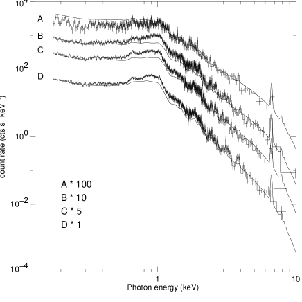
Figure 12: Spectra (solid line) synthesized from results of the best-fit hydrodynamic loop model (Fig. 7) integrated over time intervals corresponding approximately to those of the spectra shown in Paper II (intervals A to D). Data are overplotted for comparison.

There are no density-sensitive He-like triplets in the RGS band for very high temperature plasma, and therefore it is difficult to diagnose the predicted density values of the hottest flaring plasma. Available density diagnostics for this flare comes from line ratios of O VII and Ne IX groups obtained with the RGS (Paper I). The line analysis provides density values $\approx 4\times 10^{11}$ cm^-3 with a large error bar for O VII, and between $10^{11}$ and $2\times 10^{12}$ cm^-3, for Ne IX, in a time interval around the flare peak. In approximately the same time interval, the loop model yields an average density of $\approx 2\times 10^{12}$ cm^-3, and $\approx 10^{12}$ cm^-3 at the temperatures of 2 and 4 MK of maximum formation of the respective ions. For the Ne IX, the average density obtained from the model is compatible to the large interval allowed by the data, although the Ne IX derived densities are highly uncertain due to severe line blending (Paper II). The values obtained from the modeling at 2 MK are quite higher than those derived from the analysis of the O VII line. This may be motivated as follows: the O VII lines are intensely emitted both from the flaring plasma and from the remaining quiet corona. What we detect is therefore the sum of the two contributions, and the density an average of the 2 MK plasma of the flare and of the whole Prox Cen corona. If we assume an average density value of the quiet corona at 2 MK (e.g. $\sim 5\times 10^{9}$ cm^-3, compatible with the pre-flare density value shown in Paper I), we can infer the relative weight of the components contributing to form the average density value and derive an estimate of the plasma volume involved by the quiet corona component. Just to give an idea of the volumes involved, this component could be contained in a shell surrounding the whole Prox Cen star of thickness $\sim 10^{10}$ cm, i.e. of the order of the stellar radius.

From the properties of the confined plasma, we can also infer some properties of the magnetic field around the flaring structures. The pressure of the flaring plasma confined in loop A reaches values of the order of 1000 dyne cm^-2. In analogy with the derivation in Maggio et al. (2000), we find that, to keep plasma confined, a minimum magnetic field of $\sim 150$ G is required; in order to extract a total energy of $\sim 6.5\times 10^{32}$ erg in a volume of the order of $5\times 10^{29}$ cm³ and to maintain confinement, the initial non-potential magnetic field should have been at least $\sim 230$ G.

6 Final remarks

In this work we model a flare observed at a high level of detail with XMM-Newton on Proxima Centauri. The good time coverage and resolution and the high count statistics of the data has allowed us to obtain very detailed diagnostics by means of specific time-dependent hydrodynamic loop modeling. The modeling has allowed us, on the one hand to synthesize in detail a wealth of observables for comparison with data, and on the other hand to obtain a deep physical insight in the evolution and distribution of the confined plasma.

On the other hand, the constraints provided by the data allowed us to discriminate among different model choices, such as different loop lengths, the presence of more than one flaring loop, the location of the heat pulse and of the residual heating, their intensity, relative timing and timescales. This work indicates that both heating components are necessary ingredients to explain this flare, and that a second loop system, probably an arcade, is required to explain the secondary maximum.

In spite of the high degree of detail and of the many distinct trends present in the flare, relatively few model components were sufficient to match the data reasonably: a loop and an arcade of loops, all with the same length, ignited with some delay by an intense heat pulse at the footpoints and a gradual residual coronal heating. Indeed a solar flare having a similar evolution, the Bastille Day flare, indicates that the scenario of involved loops that we find is realistic. It has been recently shown that sections of the Bastille Day flare are better described with a model of several concentric loops than with a single-loop model (Reeves and Warren 2002). Our results suggest the fundamental ingredients which govern the X-ray flare evolution are the plasma confinement, a few dominant loop systems with a fixed length, and a well-defined heating function. Changes of magnetic topology within each loop system seem to have a small influence on the X-ray evolution, probably because most of them are limited to a relatively small fraction of the life of the flaring arcade (see Fig. 5 in Reeves and Warren 2002).

The loop morphology and the heating function show a well-defined pattern which may be applied to interpret other stellar flares. The heating pattern may be applied, for instance, to stellar flares with multi-slope decay (Reale 2002 and references therein) and with secondary maxima (e.g. Poletto et al. 1988, Pallavicini et al. 1990).

It will be certainly interesting also to revisit solar flares showing similar features under such perspectives and to explore the theoretical implications concerning, in particular, the flare heating mechanisms.

- (1)
- (2) Antonucci E., Dodero M. A., Peres G., Serio S., Rosner R., 1987, ApJ, 322, 522
- (3)
- (4) Arnaud, K. A. 1996, in Astronomical Data Analysis Software and Systems V, ed. G. Jacoby & J. Barnes (San Francisco: ASP), 17
- (5)
- (6) Aschwanden, M. J. & Alexander, D. 2001, Sol. Phys., 204, 91
- (7)
- (8) Betta, R. M., Peres, G., Reale, R., & Serio, S. 1997, A&AS, 122, 585
- (9)
- (10) Betta, R. M., Peres, G., Reale, F., & Serio, S. 2001, A&A, 380, 341
- (11)
- (12) Briggs K.R., & Pye J.P., 2003, A&A, in press.
- (13)
- (14) Byrne, P. B. & McKay, D. 1989, A&A, 223, 241
- (15)
- (16) den Herder, J. W. et al. 2001, A&A, 365, L7
- (17)
- (18) Doschek, G. A., Cheng, C. C., Oran, E. S., Boris, J. P., & Mariska, J. T. 1983, ApJ, 265, 1103
- (19)
- (20) Favata F., 2002, Proc. ESLAB Symposium Stellar Coronae in the Chandra and XMM-Newton Era, ESTEC, 25-29 June 2001, F. Favata, J. Drake, eds., ASP Conf. Ser. 277, 115.
- (21)
- (22) Favata F., Micela G., Reale F., 2001, A&A, 375, 485.
- (23)
- (24) Favata F., Micela G., Reale F., Sciortino S., Schmitt J. H. M. M., 2000, A&A, 362, 628
- (25)
- (26) Favata F. & Schmitt J.H.M.M., 1999, A&A, 350, 900
- (27)
- (28) Fisher, G. H., Canfield, R. C., & McClymont, A. N. 1985, ApJ, 289, 414
- (29)
- (30) Gan, W. Q., Zhang, H. Q., Fang, C., 1991, A&A 241, 618
- (31)
- (32) Golub L., Pasachoff J.M., 1997, The solar corona, Cambridge Univ. Press (Cambridge)
- (33)
- (34) Güdel, M. et al. 2001, A&A, 365, L336
- (35)
- (36) Güdel, M., Audard, M., Skinner, S. L., & Horvath, M. I. 2002, ApJL, 580, L73 (Paper I).
- (37)
- (38) Güdel, M., et al., 2003, A&A, in press (Paper II).
- (39)
- (40) Haisch B.M., 1983, in Activity in red-dwarf stars, P. B. Byrne, M. Rodonò eds, Proceedings of the Seventy-first Colloquium, Catania, Italy, August 10-13, 1982 (A83-47476 23-90) Dordrecht, D. Reidel.
- (41)
- (42) Haisch, B. M., Linsky, J. L., Bornmann, P. L., et al. 1983, ApJ, 267, 280
- (43)
- (44) Hawley S. L., et al., 1995, ApJ, 453, 464
- (45)
- (46) Hori, K., Yokoyama, T., Kosugi, T., Shibata, K., 1997, ApJ, 489, 426
- (47)
- (48) Jansen, F. et al. 2001, A&A, 365, L1
- (49)
- (50) Kopp R. A., Poletto G., 1984, Sol. Phys., 93, 351
- (51)
- (52) Maggio A., Pallavicini R., Reale F., Tagliaferri G., 2000, A&A, 356, 627.
- (53) Mason, K. O., et al. 2001, A&A, 365, L36
- (54)
- (55) Masuda, S., Kosugi, T., Hara, H., Tsuneta, S., & Ogawara, Y. 1994, Nature, 371, 495
- (56)
- (57) MacNeice, P., 1986, Sol. Phys., 103, 47
- (58)
- (59) Mewe, R., Kaastra, J. S., Liedahl, D.A., 1995, Legacy, 6, 16.
- (60)
- (61) Nagai F., 1980, Sol. Phys., 68, 351.
- (62)
- (63) Nagai, F. & Emslie, A. G. 1984, ApJ, 279, 896
- (64)
- (65) Osten R. A., Brown A., Ayres T. R., et al. 2000, ApJ, 544, 953
- (66)
- (67) Pallavicini R., Serio S., Vaiana G. S., 1977, ApJ, 216, 108
- (68)
- (69) Pallavicini R., Tagliaferri G., Stella L., 1990, A&A, 228, 403
- (70)
- (71) Peres, G., Orlando, S., Reale, F., & Rosner, R. 2001, ApJ, 563, 1045
- (72)
- (73) Peres G., Reale F., Serio S., Pallavicini R., 1987, ApJ 312, 895.
- (74)
- (75) Peres G., Rosner R., Serio S., Vaiana G. S., 1982, ApJ 252, 791.
- (76)
- (77) Pettersen B.R., 1980, A&A, 82, 53.
- (78)
- (79) Poletto G., Pallavicini R., Kopp R.A., 1988, A&A, 201, 93.
- (80)
- (81) Reale F., 2002, Proc. ESLAB Symposium Stellar Coronae in the Chandra and XMM-Newton Era, ESTEC, 25-29 June 2001, F. Favata, J. Drake, eds., ASP Conf. Ser. 277, 103.
- (82)
- (83) Reale F., Betta R., Peres G., Serio S., McTiernan J., 1997, A&A, 325, 782
- (84)
- (85) Reale F., Micela G., 1998, A&A, 334, 1028
- (86)
- (87) Reale, F., Peres, G., 1995, A&A, 299, 225
- (88)
- (89) Reale F., Peres G., Serio S., Rosner R., Schmitt J. H. M. M., 1988, ApJ, 328, 256
- (90)
- (91) Reeves, K. K., Warren, H. P., 2002, ApJ, 578, 590.
- (92)
- (93) Rosner R., Tucker W., Vaiana G., 1978, ApJ 220, 643.
- (94)
- (95) Sato J., Sawa M., Yoshimura K., Masuda S., & Kosugi T., 2003, The Yohkoh HXT/SXT Flare Catalogue, Montana State University, Bozeman (Montana, USA) & The Istitute of Space and Astronautical Science, Tokyo (Japan)
- (96)
- (97) Schmitt, J. H. M. M. & Favata, F. 1999, Nature, 401, 44
- (98)
- (99) Ségrensan D., Kervella P., Forveille T. & Queloz D., 2003, A&A, 397, L5.
- (100)
- (101) Serio, S., Peres, G., Vaiana, G. S., Golub, L., & Rosner, R. 1981, ApJ, 243, 288
- (102)
- (103) Serio S., Reale F., Jakimiec J., Sylwester B., Sylwester J., 1991, A&A, 241, 197.
- (104)
- (105) Stelzer, B. et al. 2002, A&A, 392, 585
- (106)
- (107) Strüder, L., Briel, U., Dennerl, K., et al. 2001, A&A, 365, L18
- (108)
- (109) Svestka, Z., 1976, Solar Flares, Dordrecht: Reidel, 1976,
- (110)
- (111) Sylwester B., Sylwester J., Serio S., et al., 1993, A&A, 267, 586.
- (112)
- (113) Turner, M. J. L. et al. 2001, A&A, 365, L27
- (114)
- (115) van den Oord, G. H. J., Mewe, R., 1989, A&A, 213, 245
- (116)
- (117) White, N. E., Culhane, J. L., Parmar, A. N., Kellett, B. J., Kahn, S., van den Oord, G. H. J., & Kuijpers, J. 1986, ApJ, 301, 262
- (118)