Models for the lens and source of B0218+357
A LensClean approach to determine $\mn@boldsymbol{H_{0}}$

Abstract

B0218+357 is one of the most promising systems to determine the Hubble constant from time-delays in gravitational lenses. Consisting of two bright images, which are well resolved in VLBI observations, plus one of the most richly structured Einstein rings, it potentially provides better constraints for the mass model than most other systems. The main problem left until now was the very poorly determined position of the lensing galaxy.

After presenting detailed results from classical lens modelling, we apply our improved version of the LensClean algorithm which for the first time utilizes the beautiful Einstein ring for lens modelling purposes. The primary result using isothermal lens models is a now very well defined lens position of $(255\pm 6,119\pm 4)\,$mas relative to the A image, which allows the first reliable measurement of the Hubble constant from the time-delay of this system. The result of $H_{0}=(78\pm 6)\,\text{km}\,\text{s}^{-1}\,\text{Mpc}^{-1}\ (2\,\sigma)$ is very high compared with other lenses. It is, however, compatible with local estimates from the HST key project and with WMAP results, but less prone to systematic errors. We furthermore discuss possible changes of these results for different radial mass profiles and find that the final values cannot be very different from the isothermal expectations. The power-law exponent of the potential is constrained by VLBI data of the compact images and the inner jet to be $\beta=1.04\pm 0.02$, which confirms that the mass distribution is approximately isothermal (corresponding to $\beta=1$), but slightly shallower. The effect on $H_{0}$ is reduced from the expected 4 per cent decrease by an estimate shift of the best galaxy position of ca. 4 mas to at most 2 per cent.

Maps of the unlensed source plane produced from the best LensClean brightness model show a typical jet structure and allow us to identify the parts which are distorted by the lens to produce the radio ring. We also present a composite map which for the first time shows the rich structure of B0218+357 on scales ranging from milli-arcseconds to arcseconds, both in the image plane and in the reconstructed source plane. Finally we use a comparison of observations at different frequencies to investigate the question of possible weakening of one of the images by propagation effects and/or source shifts with frequency. The data clearly favour the model of significant ‘extinction’ without noticeable source position shifts.

The technical details of our variant of the LensClean method are presented in the accompanying Paper I.

1 Introduction

The lensed B0218+357 (Patnaik et al., 1993) is one of the rapidly growing but still small number of gravitational lens systems with an accurately known time-delay (Biggs et al., 1999; Cohen et al., 2000). It is therefore a candidate to apply Refsdal’s method to determine the Hubble constant $H_{0}$ (Refsdal, 1964). Besides the time-delay and an at least partial knowledge of the other cosmological parameters, only good mass models of the lens are needed to accomplish this task. No other complicated and potentially incompletely known astrophysics enters the calculation or contributes to the errors. Since the cosmological parameters are believed to be known with sufficient accuracy now, e.g. from the WMAP project (Spergel et al., 2003), the only significant source of errors lies in the mass models themselves. The difficulties in constraining the mass distribution of lenses should not be underestimated, but the lens method is still much simpler to apply than classical distance-ladder methods, where errors difficult to estimate can enter at each of the numerous steps.

The classical methods still fight with the problem of results which are incompatible within the formal error bars. The HST key project (Mould et al., 2000; Freedman et al., 2001) e.g. obtains a value of $H_{0}=(71\pm 6)\,\text{km}\,\text{s}^{-1}\,\text{Mpc}^{-1}$ ($1\,\sigma$) which is often used as a reference. It should not be forgotten, however, that other groups obtained results which are significantly different, even though the general distance ladder used is very similar. Sandage (1999) determines a value of $53\pm 7$ ($1\,\sigma$), Parodi et al. (2000) obtain $59\pm 6$ (90 %). The differences in the analyses are various, ranging from the correction of selection effects and the Cepheid period-luminosity–relation to instrumental effects. The fact that a number of world-expert groups spent such an amount of effort but still do not agree on the final result proves how difficult the problems of distance ladder methods really are. See the references above for a discussion of possible reasons for the discrepancies. In addition we refer to Tammann et al. (2002) for an extensive discussion of this subject and an additional result of $60\pm 5$.

After finishing a first version of this paper, the analysis of the results of the first year of WMAP observations have been published. Although $H_{0}$ is not the primary goal of CMB observations, determinations of this parameter are possible with additional assumptions. Assuming an exactly spatially flat universe ($\Omega_{\mathrm{tot}}=1$) and a cosmological constant for the ‘dark energy’ (equation of state parameter $w=-1$), Spergel et al. (2003) obtain a value of $72\pm 5$. For different $w$, the result for $H_{0}$ can be significantly smaller. The assumptions of $w=1$ and $\Omega_{\mathrm{tot}}=1$ can only be dropped if additional information from other astronomical fields are included. With the local information from the 2dF Galaxy Redshift Survey (Percival et al., 2001; Verde et al., 2002), a constraint on $w$ is obtained. WMAP alone can constrain $\Omega_{\mathrm{tot}}$ only weakly, leading to wide allowed ranges for the density of dark energy or matter. For a determination of all free parameters, more astronomical data has to be included as discussed in detail by Spergel et al. (2003). The constraints for all cosmological parameters obtained from the combination of many data sets are very impressive, but it should be kept in mind that the situation now becomes similar to the distance ladder methods where model assumptions in many astrophysical fields are necessary, making realistic error estimates of the final result extremely difficult. Therefore the more parameters that go into CMB models have accurate independent determination, the better. This allows the CMB analyses to concentrate on other parameters which cannot be determined in any other way.

Taking these difficulties into account, we believe that the lens method is superior to most other methods not only in terms of the possible accuracy of $H_{0}$ but also, and not less important, in terms of estimating the possible errors reliably. We emphasize that the effort needed is small when compared with large projects like the HST key project or WMAP plus 2dF survey etc.

The only serious problem when using the lens effect to determine the Hubble constant lies in the mass models for the lenses which directly affect the resulting $H_{0}$. To be able to constrain a mass model accurately, two conditions should be met. First, the lens should be simple by which we mean the galaxy should be normal without nearby companions and without a surrounding cluster. Only in these cases can the mass distribution be described with confidence by a small number of parameters. Second, as many observational constraints as possible should be provided by the system. Advantageous is a high number of highly structured images. Extended lensed sources and Einstein rings can provide constraints for a wide range of positions and are therefore preferred to point-like multiple images. In the case of more than two images, multiple time-delays can also be used as constraints for the mass model. In addition to these pure lensing constraints, additional information from stellar dynamics or surface photometry of the lens can be included in the modelling.

Radio loud lensed sources have the potential to provide a whole set of independent observational constraints additional to those provided by optical observations. Flux ratios of the images are less affected by microlensing and extinction at radio wavelengths than optical ones. Radio observations also have the advantage that they can reach much higher levels of resolution than in the optical. Much smaller substructures in the images can therefore be detected and used for the lens models.

The lens B0218+357, discovered in the JVAS survey (Patnaik et al., 1993), meets most of the criteria for a ‘Golden Lens’ which allows an accurate determination of $H_{0}$. The lens is an isolated single galaxy, and no field galaxies nearby contribute to the lensing potential significantly (Lehár et al., 2000). The lens shows only two images of the core of the source, but substructure of the images can be used as further constraint. The main bonus is the presence of an Einstein ring which shows a lot of substructure in detailed radio maps (Biggs et al., 2001). This paper deals with utilizing the information from the ring to constrain the mass models and to determine $H_{0}$.

B0218+357 has only one disadvantage: It is the system with the smallest image separation known, which makes useful direct measurements of the lensing galaxy’s position relative to the lensed images extremely difficult. Since this parameter is of fundamental importance for the determination of $H_{0}$, no reliable results have been possible so far. Biggs et al. (1999) present a galaxy position which may be close to the correct value, but their error bars are highly underestimated as was already stated by Lehár et al. (2000).

In this paper we will first discuss ‘classical’ lens models which only use parametrized data of the compact images to constrain the models. We will see that with this approach the constraints are not sufficient to determine the galaxy position with any accuracy. To be able to determine the Hubble constant, other information has to be included which is naturally provided by the highly structured radio ring. The best method available to utilize this information is LensClean (Kochanek & Narayan, 1992). Because the method in its original form has serious shortcomings which prevent its use in a system like B0218+357, where the dynamic range between the compact images and the ring is very high, we had to improve the algorithm considerably. The LensClean method itself is discussed in Paper I (Wucknitz, 2003) while the results are presented here (Paper II).

We will use the improved version of LensClean to determine the galaxy position for isothermal models with an accuracy that is sufficient to achieve a result for the Hubble constant which is competitive with other methods but avoids their possible systematic errors. Possible deviations from isothermal mass distributions, which are the main source of systematic error when combining the results from many lenses, will be discussed by presenting a preliminary analysis of VLBI observations of the substructure of the images. These will allow us to constrain the radial mass profile for power-law models. We will learn that deviations from isothermal mass distributions do not play a major role in B0218+357, because the constraints are already quite strong and in addition the effect on $H_{0}$ is in this special case, where the galaxy position is determined indirectly with LensClean, much weaker than in most other systems. We nevertheless discuss future work which will improve the results even more.

As a secondary result we will use our best lens models and newly developed methods to produce maps of the source plane as it would look like without the action of the lens. We will show the source as well as its appearance in the lensed image plane on scales from milli-arcseconds to arcseconds.

Finally we use LensClean to shed some light on the question of scattering induced effective ‘extinction’ in the A component of B0218+357 by comparing results for data sets of different frequencies.

This Paper II as well as Paper I are condensed versions of major parts of Wucknitz (2002b). For more details the reader is referred to that work.

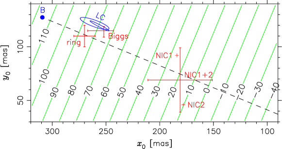
Figure 1: $H_{0}$ in units of $\mathrm{km\,s^{-1}\,Mpc^{-1}}$ as a function of galaxy position $z_{0}$ (for the concordance model, $\Omega=0.3$, $\lambda=0.3$). The dashed line connects components A (at the origin) and B. Shown are also different estimates for $\mn@boldsymbol{z}_{0}$. NIC1 and NIC2 are optical positions from Lehár et al. (2000). At the upper left are the results from Biggs et al. (1999) as well as the centre of the ring (Patnaik et al., 1993). Our final results with LensClean are shown by the ellipses (LC) to the upper left of the ‘Biggs’ error cross. These ellipses mark the formal $2\,\sigma$ uncertainties for the two parameters $x_{0}$ and $y_{0}$ with natural (smaller) and uniform (larger ellipse) weighting from Fig. 4. The $2\,\sigma$ region for the one parameter $H_{0}$ would be slightly smaller.

2 Mass models

In the absence of an accurate position of the lens relative to the position of the lensed images there is no need to use very complicated and general lens models. The effect of the lens position shows its full impact already with simple standard models. We therefore restrict most of our work to isothermal elliptical mass models. To introduce the notation, we write the lens equation as

$$\mn@boldsymbol{z_{\mathrm{s}}}=\mn@boldsymbol{z}-\mn@boldsymbol{\alpha}(\mn@boldsymbol{z})\quad\text{.}$$ (1)

The true source position $\mn@boldsymbol{z_{\mathrm{s}}}$ is the image position $\mn@boldsymbol{z}$ shifted by the apparent deflection angle $\mn@boldsymbol{\alpha}$. In static single-plane lenses, the latter can be written as gradient of a potential $\psi$:

$$\mn@boldsymbol{\alpha}(\mn@boldsymbol{z})=\mn@boldsymbol{\nabla}\psi(\mn@boldsymbol{z})$$ (2)

We use this potential to parametrize the mass models. General power-law models have

$$\psi(\mn@boldsymbol{z})=r^{\beta}\,F(\theta)\quad\text{.}$$ (3)

The radial power-law index is $\beta=1$ in the isothermal case. The arbitrary azimuthal function $F(\theta)$ describes the asymmetry. Elliptical mass distributions can be described by the formalism presented in Kormann et al. (1994) or Kassiola & Kovner (1993). We prefer the approximation of elliptical potentials (Kassiola & Kovner, 1993), which have practical advantages over the true elliptical mass distributions, because the inversion of the lens equation is possible analytically for elliptical potentials. For sufficiently small ellipticities, both approaches are equivalent. A singular elliptical power-law potential (‘SIEP’ in the isothermal case) is given by

$$\psi(\mn@boldsymbol{z})=\frac{\alpha_{0}^{2-\beta}}{\beta}\,r_{\varepsilon}(\mn@boldsymbol{z})$$ (4)

with

$$r_{\varepsilon}^{2}=\frac{x^{2}}{(1+\varepsilon)^{2}}+\frac{y^{2}}{(1-\varepsilon)^{2}}\quad\text{.}$$ (5)

For small ellipticities $\varepsilon$ and moderate $\beta$, this model corresponds to an elliptical mass distribution with axial ratio $q=1-2\varepsilon(2+\beta)/\beta$, or $q=1-6\,\varepsilon$ for isothermal models. We do not include external perturbations, because the external shear and convergence introduced by field galaxies and large scale structure are expected to be very small. Lehár et al. (2000) estimate them to be of the order $0.01$ to $0.02$, which is negligible in our context.

The time-delay $\Delta t_{i,j}$ between images $i$ and $j$ is generally related to the potential and the apparent deflection angle in the following way:

$$\Delta t_{i,j} =\frac{1+z_{\mathrm{d}}}{H_{0}}\frac{d_{\mathrm{d}}\,d_{\mathrm{s}}}{d_{\mathrm{ds}}}\Delta T_{i,j}$$ (6)

$$T_{i} =\frac{1}{2}|\mn@boldsymbol{\alpha}(\mn@boldsymbol{z}_{i})|^{2}-\psi(\mn@boldsymbol{z}_{i})$$ (7)

Here $z_{\mathrm{d}}$ is the redshift of the lens and $d_{\mathrm{d}}$, $d_{\mathrm{s}}$ and $d_{\mathrm{ds}}$ are the normalized angular size distances to the lens, source and from lens to source, respectively.

Isothermal models have an interesting analytical property, first described by Witt et al. (2000). For fixed positions of the images relative to the mass centre, the time-delay for given $H_{0}$ is uniquely determined and does not depend on any other parameters of the model, as long as the images are fitted exactly. In our case this means that, given the time-delay, $H_{0}$ for isothermal models can be calculated directly from the lens position $\mn@boldsymbol{z}_{0}$ using the equation

$$T_{i}=\frac{1}{2}|\mn@boldsymbol{z}_{i}-\mn@boldsymbol{z}_{0}|^{2}\quad\text{.}$$ (8)

The dependence of $\Delta T$ on $\mn@boldsymbol{z}_{0}$ is linear.

These simple relations show the importance of measuring the lens position directly. Once this position is known with sufficient accuracy, no explicit model fits are necessary, but the Hubble constant can be derived directly from the positions of the images and the lens.

The resulting Hubble constant for isothermal models using the time-delay of $\Delta t=10\aas@@fstack{d}5\pm 0\aas@@fstack{d}4$ (Biggs et al., 1999) is shown in Fig. 1 as a function of $\mn@boldsymbol{z}_{0}$. These values are calculated for a low-density flat universe ($\Omega=0.3$, $\lambda=0.7$). They would be smaller by 5.5 per cent for an Einstein-de Sitter universe (EdS). We use a lens redshift of $z_{\mathrm{d}}=0.6847$ (Browne et al., 1993; Carilli et al., 1993; and others) and a source redshift of $z_{\mathrm{s}}=0.944$ (Cohen et al., 2002). The older value of $z_{\mathrm{s}}=0.96$ (Lawrence, 1996) would lead to a 4.2 per cent smaller Hubble constant. Included in the plot are estimates for the lens position from different sources. The optical positions from Lehár et al. (2000) are clearly not accurate enough. The centre of the ring is relatively well defined, but it can deviate from the position of the mass centre by 0$\aas@@fstack{\prime\prime}$03 or even more, depending on the ellipticity of the lens and the size and shape of the source. We will see later that the error bars of Biggs et al. (1999) are underestimated significantly so that their result for the lens position can not be used.

The alternative time-delay of $10\aas@@fstack{d}1\pm 1\aas@@fstack{d}5$ ($2\,\sigma$) from Cohen et al. (2000) is compatible with the result from Biggs et al. (1999) which we used for our work because of the smaller error bars. The result for $H_{0}$ obtained from the Cohen et al. (2000) time-delay would be 4 per cent higher.

3 Classical isothermal lens models

Our first modelling attempts for B0218+357 followed the classical route of using only parameters of the two compact components as constraints. This is the same approach as presented in Biggs et al. (1999). We will learn that it is not possible to determine uniquely the lens position with this information. The results shown in this section were obtained using isothermal models because the (small, see below) deviations from isothermality are not of importance as long as the galaxy position is not known with high accuracy. Once this parameter is determined with LensClean, constraints on these deviations as well as the impact on $H_{0}$ will be discussed in Sec. 5.

3.1 Observational data

All coordinates in this paper are measured with respect to the A image. The $x$ coordinate is measured eastwards (increasing right ascension), $y$ is measured northwards.

Table 1 shows a compilation of known relative positions of the A and B images as well as of the subcomponents 1 and 2 which were revealed by VLBA observations (Patnaik et al., 1995). There are significant differences in the given positions, but they are too small to affect the results seriously. For the B$-$A separation, we used the 15 GHz VLBA positions for the core components A1 and B1 with their formal accuracy. The relative positions of the subcomponents offer an additional possibility to constrain the lens models. For the modelling we assumed an accuracy of 0.1 mas as in Biggs et al. (1999) and made independent calculations for the data from Patnaik et al. (1995) and Kemball et al. (2001). The difference between the two sets of positions is of the same order as the assumed error bar.

The new VLBI data presented in Biggs et al. (2003) show, in addition to the already known two close subcomponents, the inner jet in both images with subcomponents at separations of up to ca. 10 mas which could potentially provide additional constraints. These data are not used for our classical modelling because the accuracy of parametrized model fits to the additional components are influenced significantly by the underlying smooth emission of the jet. The true errors of such fits are expected to be much higher than formal estimates so that we decided to exploit this new data set only later with LensClean.

Table 1: Relative positions of components and subcomponents.

data set			$x~{}[{\text{mas}}]$	$y~{}[{\text{mas}}]$	(sub)comp
5 GHz	EVN		308.5	130.3	B$-$A
8.4 GHz	VLBI		309.00	127.30	B1$-$A1
			309.32	126.37	B2$-$A2
15 GHz	VLBA		309.2	127.4	B1$-$A1
			309.6	126.6	B2$-$A2
15 GHz	VLA		310.56	127.11	B$-$A
optical	HST		307	126	B$-$A
8.4 GHz	VLBI		1.18	0.87	A2$-$A1
			1.50	-0.06	B2$-$B1
15 GHz	VLBA		1.072	0.868	A2$-$A1
			1.470	0.000	B2$-$B1

The magnification ratio of the two compact images is more difficult to obtain. Several effects can influence the results. One problem is scattering in the lensing galaxy which seems to decrease the flux density of A. This effect is stronger for lower frequencies and (with regard to the fluxes) thought to be almost absent at 15 GHz. Secondly, flux densities of compact images embedded in a smooth surface brightness background cannot be determined unambiguously. We always have to expect an uncertainty of about the background surface brightness integrated over the beam. This error should be smaller than 10 per cent for the lower resolution data sets at lower frequencies and much less than that in other cases. Finally we observe the source at different epochs in the two images because of the time-delay. From measured light curves and the known time-delay (Biggs et al., 1999), the typical error of this effect is estimated to be less than 5 per cent.

Table 2 shows flux density ratios for different frequencies, epochs and resolutions. There seems to be a systematic increase in the ratio with increasing frequency (discounting optical), which hints at scattering. Also the spread in values for 8.4 GHz and above is relatively small. For both these reasons, and because there are values with the effects of delay removed, we chose to use a value of 3.75 which is compatible with most of the measurements at higher frequencies. Please note that the results depend only very weakly on small changes of this ratio. For the LensClean work presented below, no explicit measurement of the flux density ratio is required. Resolution effects and contamination by the ring are then taken into account automatically.

Table 2: Flux density ratio A$/$B for different frequencies and instruments.

data set				epoch	ratio
1.7	GHz	VLBI		1992 Jun 19	2.62
5	GHz	MERLIN		1991 Aug 26	2.976
5	GHz	MERLIN		1992 Jan 13	3.23
5	GHz	MERLIN		1992 Mar 27	3.35
5	GHz	EVN		1990 Nov 19	3.185
8.4	GHz	VLA		1991 Aug 1	3.247
8.4	GHz	VLA		1996/1997	3.57	$\pm 0.01$
8.4	GHz	VLA		1996/1997	3.2	$\pm 0.35$
8.4	GHz	VLBI		1995 May 9	3.18	$\pm 0.17$
					3.72	$\pm 0.20$
15	GHz	VLA		1991 Aug 1	3.690
15	GHz	VLA		1992 Nov 18	3.79
15	GHz	VLA		1996/1997	3.73	$\pm 0.01$
15	GHz	VLA		1996/1997	4.3	$\pm 0.65$
15	GHz	VLBA		1994 Oct 3	3.623	$\pm 0.065$
22	GHz	VLA		1991 Aug 1	3.636
5550 Å		HST			0.14

The subcomponents are only marginally resolved and even the formal uncertainties of fitted Gaussians are too high to serve as additional constraints. Furthermore, the apparent sizes and shapes might be influenced by scatter broadening in the interstellar medium of the lensing galaxy, which is known to be gas rich (Wiklind & Combes, 1995). We nevertheless tried to include the shapes of the subcomponents into the modelling, without any gain in accuracy of $H_{0}$. The actual observational data as given by Patnaik et al. (1995) and Kemball et al. (2001) are shown in Table 3. The fit of the best source shapes for each lens model is performed analytically with a Cartesian parametrization of the ellipses. Mathematical details can be found in Appendix A.2.

Table 3: Shapes of the subcomponents

		major axis $[{\text{mas}}]$	minor axis $[{\text{mas}}]$	p.a. $[\deg]$
A1		$0.58\pm 0.05$	$0.28\pm 0.05$	$-37$ $\pm$	5
		$1.90\pm 0.30$	$1.12\pm 0.30$	$157$ $\pm$	6
A2		$1.02\pm 0.05$	$0.54\pm 0.05$	$-47$ $\pm$	5
		$\geq 2.0$	$\geq 2.0$
B1		$0.36\pm 0.05$	$0.16\pm 0.05$	$-65$ $\pm$	15
		$0.72\pm 0.30$	$0.35\pm 0.04$	$73$ $\pm$	12
B2		$0.61\pm 0.05$	$0.23\pm 0.05$	$83$ $\pm$	10
		$\geq 0.73$	$\geq 0.73$

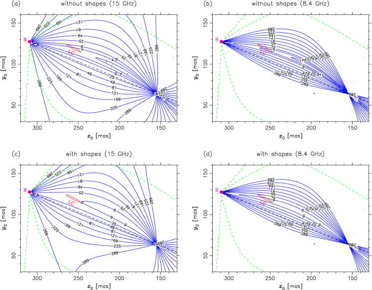
Figure 2: Best $\chi^{2}$ for isothermal models as a function of galaxy position. Subcomponent positions and shapes for the left plots are from 15 GHz VLBA data (Patnaik et al., 1995), for the right plots from 8.4 GHz VLBI data (Kemball et al., 2001). Constraints for the models are the relative position of A and B, the flux density ratio and the positions of the VLBA subcomponents. The upper plots are without, the lower ones with the subcomponent shapes included as constraints. The dashed curves separate allowed regions with two images in the central parts of the plots from regions where more than two images would be seen. The small ellipse marked LC is the $2\,\sigma$ confidence region of our final LensClean result for natural weighting, see Fig. 4 (b).

3.2 Results

Before proceeding with numerical models, we want to compare the numbers of parameters and constraints to learn what can be achieved in the absence of degeneracies. The SIEP models introduced above have a total of five free parameters (mass scale $\alpha_{0}$, position $x_{0}$, $y_{0}$ and ellipticity $\varepsilon_{x}$, $\varepsilon_{y}$), not counting the source position. The positions of A and B give us two constraints (or four constraints minus two parameters for the true source position), the flux density ratio another one. The relative positions of the subcomponents provide another two totalling in five constraints. These numbers may seem promising but we have to be aware of possible degeneracies which might prevent us from determining all parameters and $H_{0}$. This is in fact the case.

Without using the subcomponents, only three constraints are available. From this small number of constraints, it is impossible to determine the parameters of our mass model. It is in fact possible to find exactly one fitting model for each given galaxy position $\mn@boldsymbol{z}_{0}$ plotted in Fig. 1. A wide range of (positive and formally negative) values of $H_{0}$ is compatible with these data.

In the next step, we include relative positions of the subcomponents from Table 1. See Appendix A.1 for details on how these data are used in the modelling. Naively, we would expect these two more numbers to constrain the galaxy position significantly. Figure 2 (a)+(b) shows the total $\chi^{2}$ of the best fitting models for a range of fixed galaxy positions. For these models, we used a flux density ratio of 3.75, but other values measured at high frequency would lead to similar results. The relative parity of the two images was fixed to be negative as it is necessary for double image lens models. With our fitting algorithm, this was already sufficient to exclude models with more than two images in those regions where double lenses are at all possible.

As the plots show, the subcomponent positions provide only one more effective constraint, confirming the result of Lehár et al. (2000). This is easily explained. In the best models shown, the subcomponents are located nearly exactly radially with respect to the mass centre. Since singular isothermal models show no dependence of the radial stretching on image positions (there is no radial stretching at all), we lose one constraint. The only constraint left acts perpendicular to the line connecting A and B. This is unfortunately not the direction in which $H_{0}$ changes (see Fig. 1). For galaxy positions leading to realistic ranges of $H_{0}$ (like our LensClean results which will be presented later), the minimal $\chi^{2}$ is about 1.6 for the 15 GHz VLBA data (Patnaik et al., 1995) and 3.1 for the 8.4 GHz VLBI data from Kemball et al. (2001). The formal number of degrees of freedom is $\nu=0$ in this case, but the model degeneracies lead to an effective value of $\nu=1$. The fact that the data can be fitted quite well is interesting, because it shows that the data are at least approximately compatible with isothermal models.

We already noted that the shapes of the subcomponents are not a very promising candidate for further constraints. Figure 2 (c)+(d) confirms this view. The $\chi^{2}$ contribution from the shapes alone is not sensitive for shifts in the radial direction and the total $\chi^{2}$ function does not change qualitatively. The relatively high $\chi^{2}$ is a hint that the measured shapes are not exactly the correct ones, just as one might expect if the shapes are affected by scattering. The ineffectiveness of shape constraints does not change when non-isothermal models are used. This is a result of the fact that most information about the relative magnification matrix is already provided by the magnification ratio and the radial stretching of the subcomponent separations.

We conclude that the available data on the two images are compatible with lens positions leading to an extremely wide range of values of $H_{0}$ and we can therefore not confirm the relatively small error bars given by Biggs et al. (1999), even if (in contrast to Lehár et al., 2000) the subcomponent shapes are included as constraints. Without any further information about the position of the lensing galaxy, ‘classical’ lens modelling using only the compact components does not provide any useful estimates for $H_{0}$.

4 LensClean

4.1 The method

One promising way to get more information about the mass distribution of the lens is to make use of the extended emission which shows as a ring in radio maps (e.g. Biggs et al., 2001). Several approaches for models using extended emission have been discussed in the literature (e.g. Kochanek et al., 1989; Kochanek & Narayan, 1992; Ellithorpe et al., 1996; Wallington et al., 1996). They all work by, for a given lens model, constructing a map of the source which minimizes the deviations from observations when mapped back to the lens plane. The minimal residuals themselves are then used in an outer loop to find the best lens model.

In Paper I we describe the LensClean method which was first proposed by Kochanek & Narayan (1992) and Ellithorpe et al. (1996) together with a number of improvements and the details of our own implementation. The idea of LensClean as an extension of standard Clean is very simple. Clean builds up a radio map by successively collecting point sources at the peaks of the so-called dirty map, subtracting them from the observed data and in the end convolving the collection of components with a Gaussian in order to produce the Clean map. LensClean works similarly, but for each position in the source plane, emission has to be subtracted at the positions of all corresponding image positions simultaneously with the magnifications given by the (for now fixed) lens model. In this way an emission model is built which is exactly compatible with a given lens model and which comprises the best fit to the data under this assumption. An outer loop to determine the lens model parameters themselves is then built around the LensClean core. In this loop the remaining residuals of LensClean are minimized by varying the lens model parameters. The result is a combined best-fitting model for the lens mass distribution and the brightness distribution of the source.

For our work we used a data set taken at the VLA in 1992 at 15 GHz with a bandwidth of 50 MHz and a total on-source time of about 6 hours. The beam size is $129\times 146\,{\text{mas}}^{2}$ (p.a. $-73\,\degr$) with natural and $86\times 88\,{\text{mas}}^{2}$ (p.a. $-60\,\degr$) with uniform weighting. The thermal rms noise per beam is 55 $\mu$Jy for natural and 140 $\mu$Jy for uniform weighting. The same data were used in the development of LensClean described in Paper I. More details can be found there.

The standard pixel and field size used for the final runs is a $512\times 512$ pixels of $5\times 5{\text{mas}}^{2}$ each. A loop gain of $g=0.38$ is used and 5000 iterations of our improved unbiased LensClean variant are performed. Smaller pixels and a smaller loop gain would make the residual function smoother, which helps in finding the minimum, but would increase the computation times on the other hand. Systematic deviations caused by too large pixels or too high $g$ are not significant for the parameter ranges used. For the first ungridded step which removes most of the bright compact images, a loop gain of $\gamma=0.95$ is used. As magnification limit for the images we chose a value of 100.

As explained in more detail in Paper I, we scanned the range of possible lens positions $\mn@boldsymbol{z}_{0}$ and fitted the remaining lens model parameters for each position in order to stabilize the fits and to be able to determine confidence regions for the position from the final maps of residuals as a function of $\mn@boldsymbol{z}_{0}$. To reduce the remaining numerical noise, smooth polynomial functions are fitted to the residual function $R^{2}(\mn@boldsymbol{z}_{0})$ to determine the minimum and confidence regions.

Possible changes of the flux ratio A$/$B as a result of the time-delay in combination with intrinsic variability are taken into account with the methods described in Paper I. From the residuals of the best models we learned that any ratio changes have to be less than 5 per cent. This is in good agreement with monitoring data covering the epoch of our observations which showed an almost constant flux ratio of $3.79\pm 0.07$ during that time (Corbett et al., 1996). The measured flux ratio is therefore a good estimate of the true magnification ratio, almost unaffected by the combination of variability and time-delay. Taken together, these results also confirm that, even if scattering or other propagation effects in the interstellar medium (ISM) of the lensing galaxy may change the flux ratio at lower frequencies, the effect is not relevant at 15 GHz and can thus be neglected here. We will later estimate the effect at 5 GHz by comparing with our results for 15 GHz. The shifts of the best $\mn@boldsymbol{z}_{0}$ caused by flux ratio changes below 5 per cent are not significant and will be neglected.

Because of the numerical difficulties of the LensClean algorithm in combination with lens models which do not allow an analytic inversion of the lens equation, most of our calculations are done for isothermal (SIEP) models without external shear. As explained above and in Paper I, these relatively simple models are already sufficient to show the effect of the very important lens position on the determination of $H_{0}$. We will discuss later that the true radial mass profile seems to be very close to isothermal and we will estimate the effect of this deviation as a perturbation of the SIEP model.

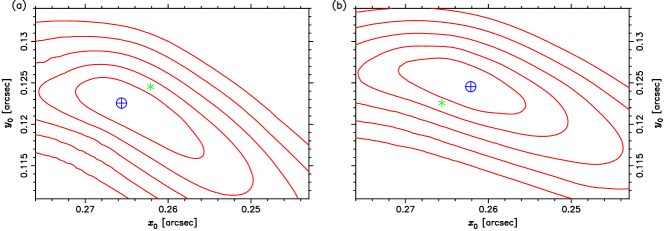
Figure 3: Final residuals for the 15 GHz VLA data set for (a) LL and (b) RR polarization (uniform weighting) for isothermal models. The results are smoothed for the contour lines (confidence limits of 1, 2, 3, 4, 5$\cdot\sigma$). The cross hair marks the respective residual minimum, the asterisks the one of the other polarization.

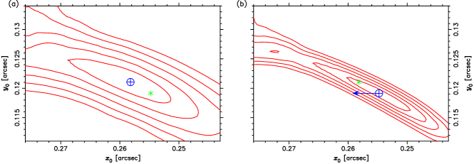
Figure 4: Final residuals for the 15 GHz VLA data set for Stokes I for isothermal models. The results are smoothed for the contour lines (confidence limits of 1, 2, 3, 4, 5$\cdot\sigma$). (a) uniform, (b) natural weighting. The cross hair marks the respective residual minima, the asterisk marks the minimum for the other weighting scheme. The arrow in (b) symbolizes the estimated shift for a non-isothermal model with $\beta=1.04$ (see Sec. 5.2). The shape of the residual function would be very similar for such a model.

4.2 Determining the lens position

We started the analysis with the left and right handed circular polarization separately to be able to use the comparison of the two as consistency check. LensClean with self-calibration as described in Paper I was used independently on the uniformly weighted LL and RR data set to produce final $uv$ data sets and residual maps. The residuals as a function of the galaxy position (relative to A) are shown in Fig. 3. To produce the plot, the residual function was interpolated and smoothed from the original results which were on a relatively coarse grid consisting of ca. 200 points.

The confidence regions are estimated from Eq. (LABEL:I-eq:DR2) in Paper I and the $\chi^{2}$ distribution as described there. The best normalized residuals are $0.77$ and $0.80$ for LL and RR, while the expectation from Eqs. (LABEL:I-eq:R2) and (LABEL:I-eq:sigma2) in Paper I would be $1\pm 0.009$. Our values are significantly lower because of the self-calibration applied to the data. We allowed independent phase and magnitude correction for each integration bin independently which, by the high number of free parameters, naturally reduces the residuals considerably. Cleaning and self-calibrating the data with DIFMAP without taking into account the lens leads to the very similar residuals of 0.78. We conclude that the best fits with LensClean have residuals within the expectations but have to keep in mind that this is not a very sensitive test for the goodness of fit. The best galaxy positions from LL and RR are clearly compatible within $1\,\sigma$.

Some care is necessary when combining the two circular polarizations to obtain total intensity I which is done in the next step. As a starting lens model for self-calibration we used the mean of the best galaxy positions for LL and RR, obtained the other parameters for this position separately for LL and RR and took the mean of the two. This provides a better estimate than taking the mean of the best models of LL and RR directly. The LensClean calculations were done as before but in the self-calibration possible differences in the calibration errors of LL and RR had to be taken into account. To do this we built the emission model for I (mean of LL and RR) and calibrated LL and RR separately with this emission model. Afterwards the two were again combined to obtain total intensity I. This standard approach relies on the assumption that no circular polarization is present and that LL and RR should (apart from noise) be the same. With uniform weighting only positive components were allowed for self-calibration. For natural weighting, we started with 3000 uniformly weighted iterations, switched to natural weighting and performed another 2000 iterations. This is superior to 5000 iterations with natural weighting because the improved resolution of the uniformly weighted beam helps in avoiding positional errors of the first bright components. Because of this weight switching, negative components were allowed as well. They are essential to compensate for the difference of uniform and natural weighting.

The results are shown in Fig. 4. The plot does not show the result from the fits directly but was produced by first fitting the models for a relatively coarse grid of $\mn@boldsymbol{z}_{0}$ with LensClean, then fitting smooth polynomials to the resulting model parameters and calculating LensClean residuals on a finer grid where the polynomial fits where used for the lens model parameters. This approach does not change the appearance of the plot but saves a large amount of CPU time because real LensClean fits have to be performed only for a much smaller number of galaxy positions than needed to produce a smooth plot.

The final error ellipses are also included in Fig. 1 and 2. Although uniform weighting was superior to natural weighting in the first stages of calibrating the data, in the end the naturally weighted results are slightly more accurate if we trust the formal statistical uncertainties. The accuracy depends on two aspects here. One is the resolution of the maps, which is better for uniform weighting, the other is the signal to noise ratio, which is optimal for natural weighting. The tradeoff between the two aspects depends on the lens models and on the data set and it is not a priori clear which weighting scheme is optimal for LensClean.

We see that the LensClean lens position is located almost exactly in the centre of the valley of low residuals of classical lens model fitting data shown in Fig. 2. The results are therefore consistent with each other. Since the two methods use very different constraints (the VLBI substructure in classical and the ring in LensClean modelling), this agreement provides good evidence that the LensClean methods actually works correctly and produces reliable results.

The statistical uncertainties in the total intensity (I) result are only slightly smaller than in the separate LL and RR results. Slightly unexpected, the best lens position from I (uniformly weighted) is not located between the best positions from LL and RR but has an offset of ca. 6 mas, still compatible within the $1\,\sigma$ bounds. This effect is not fully understood yet. It might be related to low-level circular polarization in the source which would demand a different self-calibration technique. More probable is the presence of subtle instrumental effects which could not be corrected for by self-calibration.

The final residuals for the naturally weighted data set and the best lens model are reduced $\chi^{2}=0.842$. This is again significantly below unity as a result of self-calibration. The value is compatible with results using simulated data sets but should not be used as test for the goodness of the fit. For the latter purpose we show in Fig. 5 the uniformly weighted (to increase the resolution) image space residuals for the best lens model (from uniformly weighted data) and an alternative model that is off by $1\,\sigma$ (calculated for one parameter). For these maps we used a very high number of 100 000 iterations, many more than the 5000 used for the model fits. We notice that in the outer singly imaged regions, where the Cleaning is not constrained by the lens, most of the noise has been included in the models so that the residuals are much smaller than the rms noise of the data. For the best model shown in Fig. 5 (a) even the inner parts, which really depend on the lens model, are Cleaned down to a similar level. This proves that the lens model can not be too far from the correct one. For the alternative model, on the other hand, the inner residuals are significantly higher than before, see Fig. 5 (b). These residual maps should be compared with Fig. LABEL:I-fig:resid1 (c+d) in Paper I which shows the same for a simulated data set using a known lens model. The residuals of our alternative model are of the same level as in the simulations. For the best-fitting model, the real residuals are even smaller which could be surprising at the first view but which results from the fact that the best-fitting lens model has by definition the smallest residuals which are thus always smaller than residuals for the correct lens model. We conclude that the total $uv$-space residuals and the image space residual map are both consistent with a perfect fit of the lens model.

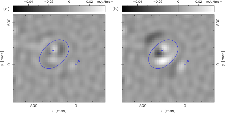
Figure 5: Uniformly weighted image plane residuals after 100 000 iterations of LensClean with (a) the best lens model, (b) a lens model that is excluded by $1\,\sigma$. The expected noise of the dirty maps is 0.14 mJy per beam. Compare these maps with their simulated equivalents in Fig. LABEL:I-fig:resid1 (c+d) of Paper I. The critical curve and the two bright images are marked.

In order to test our estimates of confidence regions in the case of uniform weighting, we performed Monte Carlo simulations the results of which are shown in Fig. LABEL:I-fig:mc in Paper I. The scatter of simulated results is in good agreement with the theoretical expectations although these could only be obtained by using approximations for the expected statistical properties of the residuals. In the case of natural weighting, the residuals follow the standard $\chi^{2}$ distribution.

4.3 Best isothermal lens model and Hubble constant

The best fitting lens models are given in Table 4. The errors are mainly due to the uncertainty in $\mn@boldsymbol{z}_{0}$. For a fixed $\mn@boldsymbol{z}_{0}$ they would be smaller by orders of magnitude. The real flux ratio calculated from the models is $3.80\pm 0.03$ which is compatible with the uniformly weighted direct model fitting to the same data set. The agreement with the value of 3.73 resulting from the time-delay analysis in Biggs et al. (1999) is also very good.

The ellipticity of the mass model is unexpectedly large. We have to remember that the ellipticity of an equivalent elliptical mass distribution is three times the ellipticity of the potential which leads to a best estimate of the axial ratio of $a/b\approx 1.4$. In contrast to this, the lensing galaxy appears quite round on optical images. The uncertainties in $\varepsilon$ are quite large, however, so the real ellipticity might be smaller. For ellipticities as high as observed here, it is of concern how far the elliptical potential still is a good approximation for elliptical mass distributions. As was shown by Witt et al. (2000), the magnification in self-similar isothermal models is a direct function of the surface mass density which means that the critical curve shown in Fig. 6 is also an isodensity contour. The shape of this curve looks rather elliptical and does not show hints of the unrealistic dumbbell shapes which are observed for more extreme ellipticities. We conclude that the use of elliptical potentials is still justified in our case.

Table 4: Parameters of the best fitting isothermal lens models for uniform and natural weighting (final result VLA 15 GHz Stokes I). The error bars are statistical $2\,\sigma$ limits for one parameter each; they originate mostly from the uncertainty of the lens position and would be much smaller for fixed $\mn@boldsymbol{z}_{0}$. The position angle of the major axis $\theta$ is measured in the usual astronomical sense from north through east.

parameter		uniform	natural
$\displaystyle\frac{1}{2}$ $x_{0}$	$[\text{arcsec}]$	$\phantom{+}0.2582\begin{smallmatrix}+0.0158\\ -0.0087\end{smallmatrix}$	$\phantom{+}0.2548\begin{smallmatrix}+0.0062\\ -0.0063\end{smallmatrix}$
$\displaystyle\frac{1}{2}$ $y_{0}$	$[\text{arcsec}]$	$\phantom{+}0.1210\begin{smallmatrix}+0.0057\\ -0.0048\end{smallmatrix}$	$\phantom{+}0.1191\begin{smallmatrix}+0.0031\\ -0.0039\end{smallmatrix}$
$\displaystyle\frac{1}{2}$ $\alpha_{0}$	$[\text{arcsec}]$	$\phantom{+}0.1616\begin{smallmatrix}+0.0039\\ -0.0124\end{smallmatrix}$	$\phantom{+}0.1634\begin{smallmatrix}+0.0026\\ -0.0034\end{smallmatrix}$
$\displaystyle\frac{1}{2}$ $\varepsilon_{x}$		$+0.0043\begin{smallmatrix}+0.0123\\ -0.0438\end{smallmatrix}$	$+0.0091\begin{smallmatrix}+0.0066\\ -0.0098\end{smallmatrix}$
$\displaystyle\frac{1}{2}$ $\varepsilon_{y}$		$-0.0707\begin{smallmatrix}+0.0273\\ -0.0637\end{smallmatrix}$	$-0.0585\begin{smallmatrix}+0.0196\\ -0.0221\end{smallmatrix}$
$\displaystyle\frac{1}{2}$ $|\varepsilon|$		$\phantom{+}0.0709$	$\phantom{+}0.0592$
$\displaystyle\frac{1}{2}$ $\theta$	$[\text{deg}]$	$-46.7$	$-49.5$
$\displaystyle\frac{1}{2}$ $\Delta T$	$[\text{arcsec}^{2}]$	$\phantom{+}0.0393\begin{smallmatrix}+0.0055\\ -0.0032\end{smallmatrix}$	$\phantom{+}0.0380\begin{smallmatrix}+0.0023\\ -0.0025\end{smallmatrix}$

The Hubble constant $H_{0}$ can now be determined from the distances and from the parameter $\Delta T$ given by the lens model. For the final result we only use the naturally weighted data since the uncertainties are smaller here. For an EdS world model, the result is $H_{0}=(74.1\pm 5.5)\,\text{km}\,\text{s}^{-1}\,\text{Mpc}^{-1}$. For a low-density flat standard model with $\Omega=0.3$ and $\lambda=0.7$, it increases by about 6 per cent:

$$H_{0}=(78.5\pm 5.8)\,\text{km}\,\text{s}^{-1}\,\text{Mpc}^{-1}$$ (9)

The error bars are formal $2\,\sigma$ limits which include the uncertainty of the lens model (6 per cent, contributed almost exclusively by the uncertainty of the lens position) and the time-delay (4 per cent). We stress that they do not include possible systematic errors which might result if the true mass distribution can not be described by our isothermal models (SIEP). As we show below, no large effects from this are expected. Using the time-delay from Cohen et al. (2000), our result becomes $H_{0}=(82\pm 13)\,\text{km}\,\text{s}^{-1}\,\text{Mpc}^{-1}$ with the largest error contribution (15 per cent) coming from the time-delay.

Standard quintessence models (e.g. Linder, 1988a, b) have parameters between the EdS and the low-density $\Lambda$ world models and would lead to Hubble constants between the two extremes. For $w=-1/3$, the result would be indistinguishable from the EdS case (equivalent to $w=0$) while for $w=-2/3$ the Hubble constant would be 2.1 per cent higher than for EdS. The cosmological constant corresponds to $w=-1$.

5 Non-isothermal lens models

It is a well known fact the the radial mass distribution is the most important source of uncertainties in the $H_{0}$–$\Delta t$ relation for lens systems where the lens position is known accurately (see e.g. references in the introduction of Kochanek, 2002a). For power-law models a simple scaling law of $H_{0}\propto 2-\beta$ is valid in many cases (Wambsganß & Paczyński, 1994; Witt et al., 1995; Wucknitz & Refsdal, 2001) while in quadruple lenses an even stronger dependence of $H_{0}\propto(2-\beta)/\beta$ was found under certain circumstances by Wucknitz (2002a) for generalized power-law models following Eq. (3). As a generalization of the SIEP models, we use elliptical power-law potentials which (if not too far from isothermal and not too elliptical) are a good approximation to elliptical power-law mass distributions. The two families of models differ only in the special form of the azimuthal function $F(\theta)$.

We will see that deviations from isothermality are very small so that our LensClean results for isothermal models can still be used as a first approximation. The deviations can thus be treated as a small perturbation.

5.1 Constraints from classical modelling

The subcomponents of both images are oriented more or less radially with respect to the expected lens position. This has the disadvantage that their positions cannot be used to constrain the galaxy position for isothermal models as shown before. For non-isothermal models, on the other hand, this insensitivity can be used to determine constraints for the radial mass profile from these data relatively independent of the true lens position. If this position is taken to be close to the LensClean result and compatible with the VLBI constraints, $\beta$ can be estimated with some accuracy using the method presented in Appendix A.1. If we use the 8.4 GHz VLBI data from Kemball et al. (2001), the result is $\beta=1.04\pm 0.02$ ($1\,\sigma$ limits). The error bar does not include uncertainties of the galaxy position but the values are relatively independent of $\mn@boldsymbol{z}_{0}$ anyway. From the 15 GHz data from Patnaik et al. (1995), a slightly larger value of $\beta=1.06\pm 0.03$ can be estimated. Biggs et al. (2003) were able to detect the jet with many subcomponents over a length of 10 mas in both images with global VLBI observations at 8.4 GHz. A systematic relative stretching of the B jet image by about 10 per cent can be accounted for by a non-isothermal lens model with $\beta\approx 1.04$, in very good agreement with the other results. We conclude that the lensing galaxy seems to be close to isothermal with a deviation in $\beta$ of only about 4 per cent, but have to keep in mind that these results are only preliminary estimates which are not based on a self-consistent lens model but used the lens position from LensClean with isothermal models to estimate deviations from isothermality. The errors of this method are expected to be only small (see also below) but a combined fit of non-isothermal lens models to the VLA and VLBI data should be aimed for in the future.

5.2 Preliminary results from LensClean

As explained in Paper I, LensClean relies on a very robust method for the inversion of the lens equation. Using the newly developed LenTil method implemented into LensClean, we were now able to perform a few tests with non-isothermal lens models. We repeated the calculations described before with the 15 GHz VLA data but used different fixed values of $\beta$ and compared the results afterwards. We noticed that the best lens position does indeed shift slightly eastwards when increasing $\beta$, by about 1 mas for 1 per cent change of $\beta$. See the arrow in Fig. 4 for an illustration. To our relief, this effect acts on $H_{0}$ in the opposite direction as the scaling with $2-\beta$, which we expect for fixed galaxy positions, so that the two cancel almost completely. A rather conservative estimate is that the $2-\beta$ scaling is reduced by at least a factor of two as a result of the shifting lens centre. This means that for a value of $\beta=1.04$ a change of the Hubble constant by at most 2 per cent is expected compared to the isothermal models. This is much smaller than the statistical uncertainties of the result for isothermal models and thus not of concern yet. When increasing $\beta$ slightly, starting from the isothermal $\beta=1$, the resulting shift of the best LensClean lens position has the tendency to decrease the optimal $\beta$ in classical fits. Combined fits of both data sets should therefore be possible and lead to very stable results.

In the near future we will use LensClean and LenTil to obtain more accurate constraints on the radial mass profile from the existing very high-quality VLBI observations at 8.4 GHz (Biggs et al., 2003). In combination with the existing VLA data which are more sensitive to the galaxy position, a self-consistent lens model can be found and accurate error estimates will be possible.

6 Source and lens plane maps

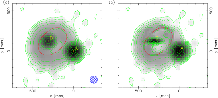
Figure 6: Lens plane maps of B0218+357. (a) Normal LensClean map at nominal resolution of the observations. The $94\times 92\,{\text{mas}}^{2}$ (p.a. $-57\degr$) restoring beam is shown at lower right. (b) Superresolved (see text). The lowest contour line in both plots is at $2\,\sigma$ of the expected noise level ($0.14\,\text{mJy}/\text{beam}$ corresponding to $1.44\cdot 10^{-8}\,\text{Jy}/{\text{mas}}^{2}$), the value doubles for each following line. The critical curve is shown as elliptical line.

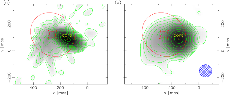
Figure 7: Source plane maps of B0218+357. (a) Restored with the anisotropic approximated source plane Clean beam (see text). (b) Restored with circular beams (similar to the lens plane beam shown at lower right). The contour levels are the same as in Fig. 6. Also shown are the diamond shaped caustic and the elliptical ‘pseudo-caustic’ or ‘cut’ (Kovner, 1987).

In Paper I we discussed a new method to reconstruct source plane maps and superresolved lens plane maps from emission models determined with LensClean. We present the resulting lens plane maps of B0218+357 in Fig. 6. One version (a) is restored with the nominal Clean beam while the other (b) is a superresolved version with anisotropic and varying beams calculated as explained in Paper I. The superresolved map is not easy to interpret because of the varying and anisotropic beams. The resolution is generally higher close to the critical curve i.e. in parts of the ring. The elliptical shape of the B Image is also a result of the local elliptical beams.

The reconstructed source plane map is shown in Fig. 7. The left map (a) is reconstructed with the source plane beams calculated from Eqs. (LABEL:I-eq:beam_source_1) and (LABEL:I-eq:beam_source_2) in Paper I. The radial streaks emerging from the region near the caustic are artifacts of the varying and highly anisotropic beams. The elliptical shape of the core is also a result of the highly eccentric local beam and should not be misinterpreted as a resolved elliptical core. The right map (b) was restored with varying but circular beams (the smallest circles which still cover the local elliptical beams completely) to make interpretations easier. Unfortunately the greatest part of the lensing magnification and improvement of resolution is lost in this map.

We see that the jet, which by coincidence emerges from the inner core in a direction very similar to the major axis of the elliptical core image in Fig. 7 (a), bends southwards and crosses the caustic of the lens at the bend. It is this part of the source which forms the ring in the lens plane and which is used as constraint by LensClean. On larger scales (shown especially well by longer wavelength observations, e.g. the 8 GHz VLA data in Fig. 8), the jet proceeds in a southern direction only to bend eastwards again at a distance of about $1\,\mathrm{arcsec}$. The jet then seemingly ends in a relatively bright blob $1.5\,\mathrm{arcsec}$ south-east of the core.

The composite colour map

in Fig. 8 shows B0218+357 on different scales both in the lens plane and in the source plane (reconstructed with LensClean). The main maps showing the outer parts of the jet on arcsec scales are made from a 8.4 GHz data set obtained at the VLA simultaneously with a global VLBI observation (Biggs et al., 2003, Fig. 4). We show a regular lens plane map and a source plane reconstruction with circular beams. The insets on the left are made from the 15 GHz VLA data set that was used for our main LensClean work. The lens and source plane maps show the same data as Fig. 6 (a) and 7 (b). We also show the critical curve in the VLA lens plane maps and the tangential caustic (diamond shape) and cut (elliptical) in the VLA source plane maps.

The insets on the right (upper: B, lower: A) are regular lens plane Clean maps of a global VLBI data set (Biggs et al., 2003). The source plane map is a projection into the source plane of the A image alone. The B image is less resolved and would not provide much additional information. The map was restored from the Clean components with the projected Clean beam. Fig. 5 in Biggs et al. (2003) shows projections of images A and B restored with equal beams to show the similarities. True LensClean source plane maps of the VLBI data have not been produced yet.

The magnifications relative to the main maps are 3 for the left insets and 130 for the jet insets on the right. The scales are the same for lens plane and source plane. The contour lines start at three times the rms noise and double for each new level. The surface brightness levels in the lens plane and source plane maps are directly comparable. The magnified sections are marked by black rectangles in the VLA maps.

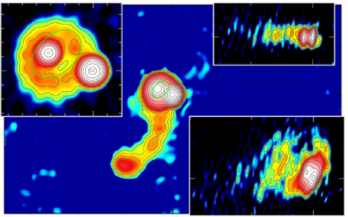
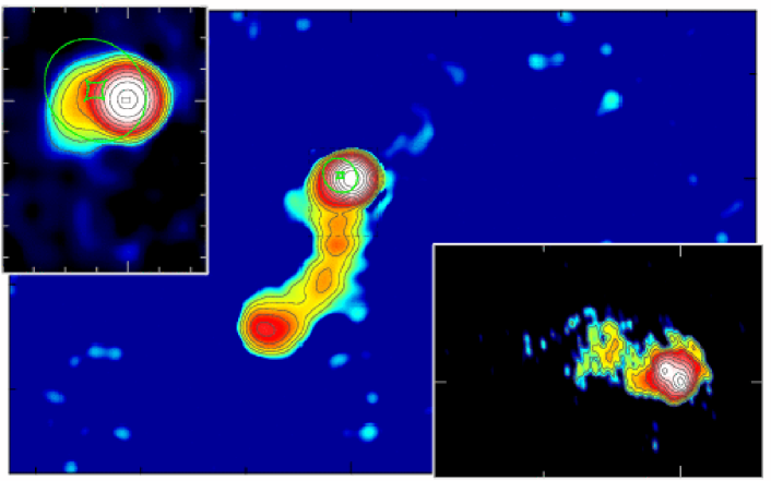
Figure 8: Composite image of the lens plane (top) and source plane (bottom) of B0218+357. The main central images show 8.4 GHz data from the VLA (tick marks 1 arcsec). The insets on the left are from the 15 GHz VLA data set (tick marks 100 mas, compare Fig. 6 and 7), the jets on the right are from 8.4 GHz global VLBI observations (tick marks 10 mas). The magnified regions are marked by black rectangles. See Section 6 on page 6 for details.

7 Investigation of frequency dependent flux ratios

It is a generally accepted fact that the apparent flux ratio A$/$B changes systematically with the frequency at which it is measured. At the high end the value seems to reach its final value of 3.8 for frequencies $\ga 15\,\text{GHz}$. On the other end the ratio goes down to 2.6 at $1.7\,\text{GHz}$ (compare Table 2). At even lower frequencies it is difficult to separate the compact emission from the ring which becomes more dominant at low frequencies. There is unambiguous evidence that the ISM of the lensing galaxy is very rich and that optical and radio emission are affected to a significant degree (Wiklind & Combes, 1995). Biggs et al. (2003) estimated the scattering measure from the broadening of image A relative to B (taking into account the magnifying effect of the lens). They obtain a value of $\text{SM}\approx 150\,\text{kpc}\,\text{m}^{-20/3}$ which is very high compared to typical lines of sight along our galaxy but comparable to lines of sight through the Galactic Centre.

One possible explanation for the low flux ratios at low frequencies is therefore the action of the very rich ISM of the lensing galaxy in front of image A. This can cause an effective extinction of A either by a high amount of scattering or by other physical effects. The refractive index of an interstellar plasma goes proportional to $\lambda^{2}$ which would explain the stronger effects for larger $\lambda$.

Another possible explanation is a very strong frequency dependence of the source structure which would effectively result in a position shift along the jet for lower frequencies. Because the spectrum of the jet is much steeper than the spectrum of the core, such an effect is not implausible. When the source is shifted in this direction, the situation becomes more symmetric and the magnification ratio decreases. For a sufficiently large shift ($\ga 10\,{\text{mas}}$) the differential magnification gradient could, in combination with this frequency dependent source position, well explain the observed flux ratio changes. There are, however, strong arguments against this scenario. If the shift is as large as required, there should be significant differences in the appearance of the innermost components in VLBI maps at 8.4 GHz (see e.g. Kemball et al., 2001; Biggs et al., 2003) and 15 GHz (see e.g. Patnaik et al., 1995), but these maps look remarkably similar. Both show two strong inner components with similar shapes and compatible relative positions. Their separation of $\sim 1.4\,{\text{mas}}$ is far too small to explain the demanded shift by different spectral indices. If the shift is caused by another component which is not seen at 15 GHz but becomes stronger at low frequencies, such a component should be detectable on a scale of $10$ to $20\,{\text{mas}}$ in the existing very deep 8.4 GHz VLBI observations. Biggs et al. (2003) do indeed detect more jet components but these are far too weak to account for a shift of the required magnitude. A more exotic alternative scenario would be refraction caused by large scale systematic trends in the column density of the lens galaxy’s ISM.

To investigate the question of extinction and/or source shifts with LensClean, we compare our best lens models fitted to the 15 GHz data which are known to be unaffected by both effects with a MERLIN data set at 5 GHz. This multi-frequency data set was used to produce the maps in Biggs et al. (2001) and is described in detail there. We used only the MERLIN part because the VLA resolution at 5 GHz is too low to be of any help here.

Unfortunately, this data set has some disadvantages for LensClean. While the resolution is better than in the 15 GHz VLA data, and the flux in the ring is higher due to the lower frequency, it was not possible to obtain reliable direct constraints for the lens model with LensClean. One problem is the possibility of extinction itself. Another very serious problem is the frequency-dependence of the emission, which is different for the ring and the compact images. Biggs et al. (2001) approximately corrected for this effect by first mapping the three frequencies independently. The Clean components responsible for the compact images were then subtracted from the data so that only the ring remains. The three data sets were rescaled in magnitude to obtain a consistent total flux density at all frequencies. Finally, the compact components from the central frequency were added back to the complete data set. This process may introduce some distortions to the lowest and highest frequencies, because it combines data for the ring from these frequencies with data for the compact components from the central frequency. The combined data were then successively mapped and self-calibrated to obtain the final data set and map.

We used the resulting $uv$ data set as basis for our computations. The spectral index correction seems to work very well for making maps, but introduces errors in LensClean which are not fully understood. This shows especially in incompatible results from the individual three frequencies and the combination of all three.

On the other hand, tests showed that the data can nevertheless be used to fit a subset of the lens model parameters if the other ones are fixed. At most three parameters can be determined accurately because they are already well defined by the two bright images alone and the ring is only a relatively small correction. We therefore used a variety of lens models compatible with the 15 GHz VLA data and fitted the same models to the 5 GHz data set allowing for a relative shift of the two data sets and a possible extinction in the A image at 5 GHz. These fits are much more robust than complete lens model fits from this data set alone. In particular, the results do not depend on which of the frequencies is used. The combination of all three also leads to the same result.

Our strategy to determine shift and extinction works like this. First we took one of the best lens models from LensCleaning the 15 GHz data. Then we fixed all parameters but $\mn@boldsymbol{z}_{0}$ and made a fit with the 5 GHz data including a (for the moment fixed) extinction in A. The difference between the two values of $\mn@boldsymbol{z}_{0}$ is then a measurement of the shift in the lens plane because in reality the lens should have the same position at both frequencies but the source may shift. We then varied the extinction to find the best value by minimizing the residuals.

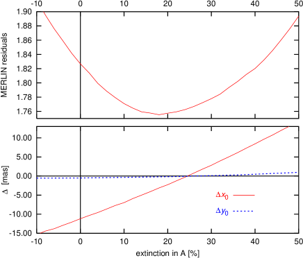
Figure 9: Fits of MERLIN 5 GHz data with lens models fitting the VLA 15 GHz data as a function of the extinction in A. top: residuals, bottom: relative shift of MERLIN$-$VLA data.

The results for one of the best VLA 15 GHz lens models are shown in Fig. 9. The position of the minimum changes somewhat when other lens models still compatible with the 15 GHz data are used. The most extreme values for the extinction are 15 and 35 per cent; most probable is a value between 20 and 30 per cent. The data sets where initially registered to obtain the same position for the A image. The relative shift in the fit (measured as a shift of the lens centre MERLIN $-$ VLA, equivalent to a shift of the source by the same amount with opposite direction) in the region of the minimum is negligible. The fact that the shifts in $x$ and $y$ have their zeros at almost the same extinction which itself is furthermore compatible with the residual minimum gives strong evidence that the real shift is indeed small and that the brightness of A at 5 GHz is reduced by $\sim 25$ per cent by some propagation effect, possibly scattering. For zero extinction, the required shift would be about $11\,{\text{mas}}$ eastwards, but the residual curve seems to be incompatible with this scenario. It seems as if extinction in A, caused by whatever physical process, accounts for a least most of the frequency dependent flux ratio. This has an important consequence for further modelling work. Although the ring becomes brighter at lower frequencies, only high frequencies can be used in a simple way to fit lens models. Observations at medium frequencies may on the other hand be used to study the propagation effects in the ISM of the lensing galaxy in more detail now that the lens model is known with sufficient accuracy.

8 Discussion

B0218+357 is one of the most promising lens systems for determining the Hubble constant with the method of Refsdal (1964). This method has, compared with other approaches, the advantage that it is a very simple one-step determination and relies on the understanding of only very little astrophysics. In this way the systematic uncertainties can not only be minimized but (equally important) also be estimated much better than in distance ladder methods which have their problems with several astrophysical processes at each step. The only serious uncertainty left is the mass distribution of the lens. In this respect B0218+357 is a close to optimal ‘Golden Lens’. The lensing galaxy seems to be a regular isolated galaxy without contributions from a group or cluster nearby. This not only avoids the inclusions of further parameters to describe the external mass distribution but also allows the assumption that the mass distribution of the galaxy itself is that of an unperturbed smooth ellipsoid. B0218+357 provides a wealth of potential constraints for the mass models in the form of highly accurate image positions, a measurable flux density ratio with probably negligible influence by microlensing, substructure on scales resolved by VLBI and a well resolved and structured Einstein ring on the scale of the image separation.

Without using the ring, ‘classical’ lens modelling allows us to tightly constrain the ellipticity and mass of the galaxy as long as its position is known. The VLBI structure of several subcomponents along the jet in a radial direction relative to the lens allows us to determine the radial mass distribution with an accuracy not possible in most other lenses (see e.g. Kochanek & Schechter, 2003, and references therein). This most important general degeneracy of the lens method can therefore be broken in the case of B0218+357. The only real disadvantage is the small size ($\sim 0\aas@@fstack{\prime\prime}3$) of the system. B0218+357 is indeed the lens with the smallest image separation known to date. Although the images and the lens are detected with optical observations, it was until now not possible to use these observations to accurately measure the galaxy position directly. HST/ACS observations obtained recently are currently analysed to allow a first useful direct measurement.

The model lens positions from Biggs et al. (1999) are probably not too far from the truth and are indeed consistent with our results but their error bars are seriously underestimated. We have shown that, without using the ring, no useful estimate of the galaxy position and thus $H_{0}$ is possible.

Previous efforts have not utilized the most striking feature of B0218+357, the beautiful Einstein ring shown by radio observations (e.g. Biggs et al., 2001). Doing this is much more difficult than using parameters of compact components because the source itself has to be modelled as well, either implicitly or explicitly. The method best suited for this task is LensClean which surprisingly has been used only for very few cases before. This is partly a result of the high numerical demands and partly of serious shortcomings of the original method as it was implemented by Kochanek & Narayan (1992) and Ellithorpe et al. (1996). In Paper I we discuss the development of our new improved variant of LensClean. One of the most important improvements is the implementation of a new unbiased selection of components.

The problem of determining the lens position is almost degenerate because the bright components, which contribute most of the signal, provide no information for this parameter. It is only the relatively weak and fuzzy ring which can be used as constraint. In other words the residuals have a very strong dependency on two directions (defined by the compact components) of the five dimensional parameter space but change only weakly in the other three directions as a result of the constraints provided by the ring. Finding minima of functions like this is a numerically difficult problem and relies on the very accurate knowledge of the residual function. Any numerical noise produces local minima which make the finding of the global minimum difficult. Special care was therefore needed to produce the best possible results with the given limited computing resources.

The modified LensClean algorithm was applied to a 15 GHz VLA data set resulting in good constraints for all parameters of an isothermal lens model, including the lens position of $x_{0}=(255\pm 6)\,$mas, $y_{0}=(119\pm 4)\,$mas relative to the A image. This model was then used to determine the Hubble constant from the time-delay of Biggs et al. (1999) to be $H_{0}=(78\pm 6)\,\text{km}\,\text{s}^{-1}\,\text{Mpc}^{-1}$. The error bars are $2\,\sigma$ confidence limits which for the Hubble constant include the error of the lens position (6 per cent) and the time delay (4 per cent). The accuracy for all other lens model parameters is much higher as long as the position is fixed. The value for $H_{0}$ is in agreement with the results from the HST key project (Mould et al., 2000; Freedman et al., 2001) and the WMAP project (Spergel et al., 2003) but incompatible with the lower distance-ladder results of Sandage (1999), Parodi et al. (2000) or Tammann et al. (2002).

Recently, a series of papers was published by Kochanek (2002a, b, 2003), see also Kochanek & Schechter (2003), in which it is claimed that a number of gravitational lens time-delays is compatible with the Hubble constant from the HST key project only if the mass concentration is as compact as the light distribution ($\beta<1$ in the picture of power-law models). Our result for B0218+357 does not confirm this view and does not give rise to a ‘new dark matter problem’ since it is significantly higher than other results from lenses. Our isothermal models lead to a value absolutely compatible with the one preferred in Kochanek (2002a). One could now in a similar way compare with the lower $H_{0}$ results of Sandage (1999), Parodi et al. (2000) or Tammann et al. (2002). However, as long as the local determinations do not agree with each other, we consider such an exercise to be of only limited value.

Rather than using locally measured values for $H_{0}$ to constrain lens mass distribution, we prefer a more direct approach, either using the lens effect itself (see below), or by including additional information. The latter approach is followed by thy ‘Lenses Structure and Dynamics’ survey LSD (Koopmans & Treu, 2002; Treu & Koopmans, 2002b, a; Koopmans & Treu, 2003a; Koopmans et al., 2003; Koopmans & Treu, 2003b). The general idea is simple: The total mass within the Einstein radius is well constrained by lensing, in contrast to the radial mass profile. For the given mass, the stellar velocity dispersion of the lensing galaxy depends strongly on this profile. The more the mass is concentrated in the centre, the deeper the potential well and the higher the velocity dispersion has to be. With some additional assumptions, it is indeed possible to obtain valuable constraints which can then again be included in the lens models to determine $H_{0}$. For the important system PG 1115+080, Treu & Koopmans (2002b) obtain a power-law index of $\beta=0.65$ which increases the otherwise very low estimate of $H_{0}$ for this system to a value of $59\pm 10$ ($1\,\sigma$). This steep mass profile is quite unusual and moves the galaxy significantly off the fundamental plane. Nevertheless it is not as steep as the light profile and the result for $H_{0}$ correspondingly lies between the isothermal and constant $M/L$ model results of Kochanek & Schechter (2003). For B1608+656, Koopmans et al. (2003) are able to constrain the mass profile of the main lensing galaxy quite well and find that it is consistent with isothermal. The resulting Hubble constant is $75\pm 7$ ($1\,\sigma)$, inconsistent with the very low mean value of $48\pm 3$ obtained by Kochanek (2002b, 2003) for isothermal models for a number of lenses, but consistent with our result for B0218+357. However, B1608+656 has the major disadvantage of a second lensing galaxy very close to the primary. The two galaxies might even be interacting which could cause complicated deviations from usual galaxy mass distributions.

These examples show that the general picture of lensing constraints for $H_{0}$ and mass profiles is not as consistent as it appeared not long ago (e.g. Koopmans & Fassnacht, 1999). In our opinion the only way to resolve the discrepancies is to try and use the best available constraints for all applicable lens systems individually. Our work on B0218+357 shows this for one example, although there are still many open questions.

Our alternative way of constraining mass profiles relies on the lens effect alone and has the advantage that additional astrophysics (galactic dynamics in LSD work) and corresponding additional model assumptions are not needed, keeping the method simple and clean. It is easy to understand that lenses showing only two or four images of one compact source cannot provide sufficient information to constrain the mass profile tightly, especially since quads usually have all images close to the Einstein ring so that they probe the potential at only one radius. Far better suited are systems with extended sources or at least with substructure in the compact images. B0218+357 is a good example which offers both.

Using our galaxy position as an estimate, non-isothermal power-law models could be constrained with the VLBI substructure. These are not the final results since no self-consistent fitting of all available data has been performed so far, but the weak dependency of the radial mass exponent $\beta$ on the galaxy positions shows that the estimate is nevertheless quite good. We learned that the mass distribution in the lens is close to isothermal (which would be $\beta=1$) but is slightly shallower ($\beta\approx 1.04$). Preliminary calculations with LensClean showed that the shift in the best lens position caused by this small deviation partly compensates for the expected scaling with $2-\beta$ for a fixed position. We therefore do not expect very significant changes of the result for $H_{0}$ from the slight non-isothermality in this system. A very conservative error estimate disregarding this compensation effect would be a possible 4 per cent error for $H_{0}$.

It has to be kept in mind, however, that all results presented so far depend on the assumption of a power-law for the mass profile (and potential and deflection angle). For more general mass models the constraints on $\beta$ are still interesting, but they only measure the local slope of the profile rather than the global mass profile. It is expected that power-laws can be used as a very good approximation for more general models for limited ranges of radii, and our model fits confirm this view in the case of B0218+357. The LensClean results for the lens position presented here are therefore also valid for other mass profiles, but the value for the Hubble constant may well have to be modified slightly.

The mass models discussed here do not include external shear because it seems to be very small. The expected true external shear of 1–2 per cent (Lehár et al., 2000) would change the result of $H_{0}$ by about the same amount at most. More difficult to estimate is the possible influence of differences in the ellipticity of the inner and outer parts of the lensing galaxy which can effectively also act as external shear. The possible impact of the remaining higher-order aspects of the mass profile degeneracies and the effects of multi-component mass models (bulge+disc+halo) are currently under investigation, especially the aspect of what apparent isothermality in the central part of the galaxy, which should be dominated by the luminous matter in the bulge, means for the true mass distribution.

In the future we will avoid the model fitting of VLBI components which are then used as constraints and instead use LensClean itself also on the existing VLBI data that show a wealth of structure in the images (see Fig. 8). To be able to use non-isothermal models with LensClean, we developed the new method LenTil for the inversion of the lens equation. With these two methods combined, a simultaneous fit of medium resolution VLA data (sensitive to the lens position) and the existing high resolution VLBI data of Biggs et al. (2003), which are more sensitive to the radial mass profile, will not only improve the results for all parameters but will, by using self-consistent lens models, also provide realistic error estimates including all uncertainties.

To be able to use the 8.4 GHz data set it will be necessary to include the extinction and scatter broadening in the A image in the models. This is possible because the 15 GHz data are only little affected by extinction so that the combination of the two allows estimates of this effect. Since the VLBI constraints for the lens models are mainly given by the positions of subcomponents but not by their size, which is relatively independent of the lens model, the different sizes of components in A and B can be used to obtain better constraints on the scattering measure than the simple estimates from Biggs et al. (2003).

The application of LensClean to the VLBI data will also show whether any significant amount of substructure in the mass distribution of the lens is needed to explain all features of the jet. The first results from Biggs et al. (2003) seem to be compatible with no substructure, but a quantitative analysis can be done in the future. If significant substructure effects are present, it will also be necessary to correct the medium resolution data for them before using LensClean to determine the galaxy position. Clumps of matter close to one of the images could change the magnification significantly which would then mimic a different lens model. The analysis of the VLBI data will show whether this may be the explanation for the (compared with some other lenses) relatively high result for $H_{0}$. LensClean can also be used to study substructure from VLBI observations of other lenses. It will then be possible to do an analysis similar to e.g. Metcalf (2002) but without any assumption about the true source structure.

To improve the medium resolution side, we recently performed observations of B0218+357 at 15 GHz using the fibre link between the VLA and the VLBA telescope Pie Town. This combination provides a resolution 1.5–2 times better than the VLA alone. The long track observation of the total accessible hour angle range of 14 hours also improves the sensitivity which in combination with the improved resolution can reduce both statistical and (even more important) systematical errors. Simulations performed before the observations showed that an accuracy of about 1–2 mas for the lens position should be achievable. This would in comparison to the existing data be an improvement of a factor of $\sim 5$. The remaining uncertainty in $H_{0}$ from the lens position alone will then shrink to below 2 per cent. Possible uncertainties caused by calibration errors will also be reduced significantly. This new data set is currently being calibrated and will be analysed with LensClean soon, alone and in combination with the VLBI data.

As a secondary result of LensClean we presented maps of the brightness distribution of the source as well as improved lens plane maps, both produced with a method newly developed together with LensClean in Paper I. This allowed the first view of B0218+357’s source as it would be seen without the distortion of the lens, but with improved resolution. The ring itself is caused by a bending jet which crosses the tangential caustic of the lens. In the future we will improve these results and also produce source plane polarization maps. The ring shows an interesting radial polarization pattern (Biggs et al., 2003) and the data will, when projected to the source plane, give us a very detailed and magnified view of the polarization structure in the jet of the source.

Finally we used LensClean to investigate the puzzling changes of the flux density ratio A$/$B with frequency. To test the two theories of either scattering induced extinction caused by the ISM in the lensing galaxy or of an effective shift of the source with frequency, we compared our best LensClean models, which were fitted to 15 GHz data where the fluxes are expected to be unaffected by propagation effects, with MERLIN data at 5 GHz taking into account a possible relative shift and extinction in the 5 GHz data. Although the 5 GHz data set has some calibration problems, the evidence for a significant extinction ($\sim 25$ per cent) of the A component at 5 GHz is very strong. The relative shift of the source between these two frequencies seems to be negligible. This work will be extended in the future by comparing medium resolution data sets at different frequencies in order to study the propagation effects in the lensing galaxy in more detail. Observations with MERLIN at different frequencies will allow us to measure the position dependent Faraday rotation and depolarisation, providing invaluable information about the ISM of the lensing galaxy.

A direct measurement of the galaxy position in B0218+357 by HST/ACS observations will be available soon. The formal uncertainty of this measurement may be larger than the LensClean model constraints but it will be an absolutely independent and therefore complementary direct measurement. The comparison will either confirm the lens models or give information about deviations of the true mass distribution from the relatively simple models. We will then reach the point were the uncertainty in $H_{0}$ is no longer dominated by the lens models but by the time-delay uncertainties themselves. A reanalysis of existing monitoring data (Biggs et al., 1999; Cohen et al., 2000) and new monitoring campaigns will therefore allow further improvements. With all the constraints available now or soon and the simplicity of the possible mass models, B0218+357 has the potential to lead to the most robust measurement of $H_{0}$ of all time-delay lenses.

Appendix A Using the subcomponents as model constraints

Applying the lens equation (1) for two nearby positions gives to first order:

$$\Delta\mn@boldsymbol{z_{\mathrm{s}}}={\textbf{{M}}}^{-1}\Delta\mn@boldsymbol{z}$$ (10)

Here M denotes the magnification matrix

$$({\textbf{{M}}}^{-1})_{ij}=\delta_{ij}-\frac{\partial\alpha_{i}}{\partial z_{j}}\quad\text{.}$$ (11)

Clearly any information about the small scale structure of the images A and B (flux density ratio, subcomponent positions and shapes) can only provide constraints for the relative magnification matrix ${\textbf{{M}}}_{\mathrm{A}}^{-1}\,{\textbf{{M}}}_{\mathrm{B}}^{\vphantom{jkl^{\prime}m}}$.

A.1 Relative Positions

It would be possible to use the subcomponents of A and B as images of two independent sources to constrain the models in the usual way. Since the separation of the subcomponents is much smaller than the typical scale of the system, however, these data can only constrain the first derivative of the deflection angle, i.e. the magnification matrix. A different approach to constrain this matrix directly is therefore more appropriate.

Given a model value for the relative position vector of $\bar{\mn@boldsymbol{r}}_{\mathrm{s}}$ in the source plane, the corresponding vectors in the lens plane are given by Eq. (10), leading to a contribution to $\chi^{2}$ of

$$\chi^{2}=\sum_{i=\mathrm{A,B}}{\bigl{(}\mn@boldsymbol{r}_{i}-{\textbf{{M}}}_{i}\bar{\mn@boldsymbol{r}}_{\mathrm{s}}\bigr{)}}^{\dagger}\,{\textbf{{C}}}_{i}^{-1}\,\bigl{(}\mn@boldsymbol{r}_{i}-{\textbf{{M}}}_{i}\bar{\mn@boldsymbol{r}}_{\mathrm{s}}\bigr{)}$$ (12)

with the measured lens plane vectors of $\mn@boldsymbol{r}_{\mathrm{A}}$, $\mn@boldsymbol{r}_{\mathrm{B}}$ and corresponding covariance matrices ${\textbf{{C}}}_{\mathrm{A}}$ and ${\textbf{{C}}}_{\mathrm{B}}$. This equation defines an ordinary linear least squares problem leading to a weighted mean of the backprojected $\mn@boldsymbol{r}_{i}$ for the solution:

$$\bar{\mn@boldsymbol{r}}_{\mathrm{s}}=\left(\sum_{i=\text{A,B}}{\textbf{{M}}}_{i}{\textbf{{C}}}_{i}^{-1}{\textbf{{M}}}_{i}\right)^{-1}\,\sum_{i=\text{A,B}}{\textbf{{M}}}_{i}{\textbf{{C}}}_{i}^{-1}\,\mn@boldsymbol{r}_{i}$$ (13)

A.2 Shapes and sizes

With the common polar ellipticity parameters, fits can only be done numerically and are potentially very unstable. The following Cartesian formalism allows a direct analytical fit for the elliptical shape of the source to minimize the deviations from the observed images. An ellipse with major and minor axis $a$ and $b$ with direction of the major axis $\phi$ (mathematical sense) can be described by the matrix E. For all points $\mn@boldsymbol{x}$ located on the ellipse, the following equation holds:

$${\mn@boldsymbol{x}}^{\dagger}{\textbf{{E}}}^{-1}\mn@boldsymbol{x}=1$$ (14)

$${\textbf{{E}}}=\begin{pmatrix}R_{+}+R_{-}\cos 2\phi&R_{-}\sin 2\phi\\ R_{-}\sin 2\phi&R_{+}-R_{-}\cos 2\phi\end{pmatrix}$$ (15)

$$R_{+} =\frac{a^{2}+b^{2}}{2}$$ (16)

$$R_{-} =\frac{a^{2}-b^{2}}{2}$$ (17)

The astronomical position angle (north through east) is related by $\mbox{p.a.}=\pi/2-\phi$. Transformation between source and lens plane is linear for the ellipticity parameters $E_{ij}$:

$${\textbf{{E}}}_{\mathrm{s}} ={\textbf{{M}}}_{\mathrm{A}}^{-1}{\textbf{{E}}}_{\mathrm{A}}{\textbf{{M}}}_{\mathrm{A}}^{-1}$$ (18)

$$={\textbf{{M}}}_{\mathrm{B}}^{-1}{\textbf{{E}}}_{\mathrm{B}}{\textbf{{M}}}_{\mathrm{B}}^{-1}$$ (19)

We can therefore use the same simple general linear least squares formalism as in Appendix A.1 with transformation matrices for the three-dimensional ellipticity vector $(R_{+},R_{-}\cos 2\phi,R_{-}\sin 2\phi)$. In this way the best source plane ellipticity matrix/vector and the residual contributions can be calculated analytically. The Cartesian approach also avoids singularities and degeneracies for certain shapes, e.g. for circular sources.

References

- Biggs et al. (1999) Biggs A. D., Browne I. W. A., Helbig P., Koopmans L. V. E., Wilkinson P. N., Perley R. A., 1999, MNRAS, 304, 349
- Biggs et al. (2001) Biggs A. D., Browne I. W. A., Muxlow T. W. B., Wilkinson P. N., 2001, MNRAS, 322, 821
- Biggs et al. (2003) Biggs A. D., Wucknitz O., Porcas R. W., Browne I. W. A., Jackson N., Mao S., Patnaik A. R., Wilkinson P. N., 2003, MNRAS, 338, 599
- Browne et al. (1993) Browne I. W. A., Patnaik A. R., Walsh D., Wilkinson P. N., 1993, MNRAS, 263, L32
- Carilli et al. (1993) Carilli C. L., Rupen M. P., Yanny B., 1993, ApJ, 412, L59
- Cohen et al. (2000) Cohen A. S., Hewitt J. N., Moore C. B., Haarsma D. B., 2000, ApJ, 545, 578
- Cohen et al. (2002) Cohen J. G., Lawrence C. R., Blandford R. D., 2002, ApJ, in print, also available as astro-ph/0209457
- Corbett et al. (1996) Corbett E. A., Browne I. W. A., Wilkinson P. N., 1996, in Kochanek & Hewitt (1996), p. 37
- Ellithorpe et al. (1996) Ellithorpe J. D., Kochanek C. S., Hewitt J. N., 1996, ApJ, 464, 556
- Freedman et al. (2001) Freedman W. L., et al., 2001, ApJ, 553, 47
- Kassiola & Kovner (1993) Kassiola A., Kovner I., 1993, ApJ, 417, 450
- Kemball et al. (2001) Kemball A. J., Patnaik A. R., Porcas R. W., 2001, ApJ, 562, 649
- Kochanek (2002a) Kochanek C. S., 2002a, ApJ, submitted, also available as astro-ph/0204043
- Kochanek (2002b) Kochanek C. S., 2002b, ApJ, 578, 25
- Kochanek (2003) Kochanek C. S., 2003, ApJ, 583, 49
- Kochanek et al. (1989) Kochanek C. S., Blandford R. D., Lawrence C. R., Narayan R., 1989, MNRAS, 238, 43
- Kochanek et al. (2002) Kochanek C. S., Falco E. E., Impey C., Lehár J., McLeod B., Rix H.-W., , 2002, CASTLeS website, http://cfa-www.harvard.edu/castles/
- Kochanek & Hewitt (1996) Kochanek C. S., Hewitt J. N., eds, 1996, Astrophysical Applications of Gravitational Lensing IAU Symp. 173
- Kochanek & Narayan (1992) Kochanek C. S., Narayan R., 1992, ApJ, 401, 461
- Kochanek & Schechter (2003) Kochanek C. S., Schechter P. L., 2003, in Freedman W. L., ed., Measuring and Modeling the Universe, Carnegie Observatories Astrophysics Series, Vol. 2. in print, also available as astro-ph/0306040 The Hubble Constant from Gravitational Lens Time Delays
- Koopmans & Fassnacht (1999) Koopmans L. V. E., Fassnacht C. D., 1999, ApJ, 527, 513
- Koopmans & Treu (2002) Koopmans L. V. E., Treu T., 2002, ApJ, 568, L5
- Koopmans & Treu (2003a) Koopmans L. V. E., Treu T., 2003a, astro-ph/0308056
- Koopmans & Treu (2003b) Koopmans L. V. E., Treu T., 2003b, ApJ, 583, 606
- Koopmans et al. (2003) Koopmans L. V. E., Treu T., Fassnacht C. D., Blandford R. D., Surpi G., 2003, astro-ph/0306216
- Kormann et al. (1994) Kormann R., Schneider P., Bartelmann M., 1994, A&A, 284, 285
- Kovner (1987) Kovner I., 1987, ApJ, 312, 22
- Lawrence (1996) Lawrence C. R., 1996, in Kochanek & Hewitt (1996), p. 299
- Lehár et al. (2000) Lehár J., et al., 2000, ApJ, 536, 584
- Linder (1988a) Linder E. V., 1988a, A&A, 206, 175
- Linder (1988b) Linder E. V., 1988b, A&A, 206, 190
- Metcalf (2002) Metcalf R. B., 2002, ApJ, 580, 696
- Mould et al. (2000) Mould J. R., et al., 2000, ApJ, 529, 786
- Parodi et al. (2000) Parodi B. R., Saha A., Sandage A., Tammann G. A., 2000, ApJ, 540, 634
- Patnaik et al. (1993) Patnaik A. R., Browne I. W. A., King L. J., Muxlow T. W. B., Walsh D., Wilkinson P. N., 1993, MNRAS, 261, 435
- Patnaik & Porcas (1999) Patnaik A. R., Porcas R. W., 1999 Frequency dependent radio structure of the gravitational lens system B0218+357. ASP Conf. Ser. 156, p. 247
- Patnaik et al. (1995) Patnaik A. R., Porcas R. W., Browne I. W. A., 1995, MNRAS, 274, L5
- Percival et al. (2001) Percival W. J., et al., 2001, MNRAS, 327, 1297
- Refsdal (1964) Refsdal S., 1964, MNRAS, 128, 307
- Sandage (1999) Sandage A., 1999, ApJ, 527, 479
- Spergel et al. (2003) Spergel D. N., et al., 2003, ApJS, 148, 175
- Tammann et al. (2002) Tammann G. A., Reindl B., Thim F., Saha A., Sandage A., 2002, in Metcalfe N., Shanks T., eds, A New Era in Cosmology Cepheids, supernovae, , and the age of the universe, also available as astro-ph/0112489. ASP Conf. Ser. 283
- Treu & Koopmans (2002a) Treu T., Koopmans L. V. E., 2002a, ApJ, 575, 87
- Treu & Koopmans (2002b) Treu T., Koopmans L. V. E., 2002b, MNRAS, 337, L6
- Verde et al. (2002) Verde L., et al., 2002, MNRAS, 335, 432
- Wallington et al. (1996) Wallington S., Kochanek C. S., Narayan R., 1996, ApJ, 465, 64
- Wambsganß & Paczyński (1994) Wambsganß J., Paczyński B., 1994, AJ, 108, 1156
- Wiklind & Combes (1995) Wiklind T., Combes F., 1995, A&A, 299, 382
- Witt et al. (2000) Witt H. J., Mao S., Keeton C. R., 2000, ApJ, 544, 98
- Witt et al. (1995) Witt H. J., Mao S., Schechter P. L., 1995, ApJ, 443, 18
- Wucknitz (2002a) Wucknitz O., 2002a, MNRAS, 332, 951
- Wucknitz (2002b) Wucknitz O., 2002b, PhD thesis, Universität Hamburg, Germany, available from the author or from http://www.astro.physik.uni-potsdam.de/~olaf/
- Wucknitz (2003) Wucknitz O., 2003, MNRAS, also available as astro-ph/0312262 (Paper I)
- Wucknitz & Refsdal (2001) Wucknitz O., Refsdal S., 2001, in Brainerd T. G., Kochanek C. S., eds, Gravitational Lensing: Recent Progress and Future Goals, ASP conf. series, Vol. 237 Degeneracies of the radial mass profile in lens models. p. 157