LensClean revisited

Abstract

We discuss the LensClean algorithm which for a given gravitational lens model fits a source brightness distribution to interferometric radio data in a similar way as standard Clean does in the unlensed case. The lens model parameters can then be varied in order to minimize the residuals and determine the best model for the lens mass distribution. Our variant of this method is improved in order to be useful and stable even for high dynamic range systems with nearly degenerated lens model parameters. Our test case B0218+357 is dominated by two bright images but the information needed to constrain the unknown parameters is provided only by the relatively smooth and weak Einstein ring. The new variant of LensClean is able to fit lens models even in this difficult case. In order to allow the use of general mass models with LensClean, we develop the new method LenTil which inverts the lens equation much more reliably than any other method. This high reliability is essential for the use as part of LensClean. Finally a new method is developed to produce source plane maps of the unlensed source from the best LensClean brightness models. This method is based on the new concept of ‘dirty beams’ in the source plane.

The application to the lens B0218+357 leads to the first useful constraints for the lens position and thus to a result for the Hubble constant. These results are presented in an accompanying Paper II, together with a discussion of classical lens modelling for this system.

1 Introduction

The subject of gravitational lensing has matured from a curiosity and test of the theory of general relativity to an invaluable tool for a wide area of astrophysical applications, ranging from cosmology down to the study of compact objects within our own galaxy. One of the most important cosmological applications is the determination of the Hubble constant from time-delays between multiple images of lensed extragalactic sources as proposed by Refsdal (1964). The idea is simple: By measuring image positions and making model assumptions for the mass distribution, the general geometry of a given lens system can be determined. With the determination of only one length in this geometry, all other lengths, especially the distances to the lens and source, can immediately be deduced, thus allowing the determination of $H_{0}$ from the measured redshifts. The essential length can be provided by measurements of the light travel time difference (‘time-delay’) between two images of the same source. The method does not rely on the understanding of complicated astrophysical processes but only on the validity of the static weak-field limit of general relativity, which is confirmed by numerous tests, and on the Friedmann–Robertson-Walker cosmological model.

The only critical topic is the mass distribution of the lens in question. Using simple models like singular isothermal ellipsoidal mass distributions, the constraints provided by the image geometry are sufficient to determine the model parameters for many lens systems with high accuracy. Unfortunately results obtained in this way are very model-dependent and may thus be biased by astrophysical prejudice. The geometry of multiply imaged point sources can naturally not provide a sufficient number of constraints to determine the parameters of more general model families. In order to overcome the difficulty, more information has to be included in the modelling. This can be achieved by using multiply imaged extended sources in which each sub-component of the source provides its own set of constraints.

Extragalactic sources do generally show more structure at radio wavelengths than in the optical, which is an important motivation to concentrate on radio lenses. Additionally the use of radio interferometers of different sizes at different wavelengths allows the study on scales from below milli-arcseconds to above arcminutes. Even with the most modern telescopes this is not possible at optical wavelengths.

In the case of well-resolved and separated multiple subcomponents, the standard approach of first measuring the positions, flux densities and shapes of the subcomponents and using these parameters for the modelling works very well. In the general case, however, the structure of radio sources cannot be parametrized in a simple way. Several approaches for models using extended emission without parametrizing the source have been proposed in the literature which all follow the same general concept. For a given lens model they construct a map of the source which minimizes the deviations from observations when mapped back to the lens plane. The minimal residuals themselves are then used in an outer loop to find the best lens model.

The first and most simple method we tried is the so called ring cycle (Kochanek et al., 1989). It is based on pixellated maps of the true lensed surface brightness of the system. For each pixel in the source plane, a mean of corresponding surface brightnesses in the lens plane is calculated. The scatter in these pixels can be combined to get a meaningful measure for the deviation of the observations from the best model map. The weakness of this algorithm is its dependence on the true surface brightness. Optical and radio data always provide maps which are a convolution of the true brightness distribution with the point spread function (optical) or the dirty beam (radio). One might think of deconvolving these maps to get a more accurate estimate of the true image, but this process always introduces artifacts and biases which will show as difficult to interpret errors in the final results. This is a typical inverse problem and it is much better to apply the well understood effects of the observational process on the model data to compare directly with the observations than to do it the other way round and try to correct the observations to compare with the model.

For the problem of lens modelling with radio data, this leads directly to the LensClean algorithm which was introduced by Kochanek & Narayan (1992) and Ellithorpe et al. (1996). We do not use LensMEM (Wallington et al., 1996), which is a formulation of the classical maximum entropy method for a lensed situation, because the regularisation with an entropy term changes the residuals in a way which is difficult to interpret statistically. Since we rely on the residuals to determine the best lens models, we prefer to avoid such effects.

In this paper we describe a number of improvements of the original LensClean method. The motivation to start the development of our own implementations was the study of the radio lens system B0218+357 (Patnaik et al., 1993) which has a measured time-delay (Biggs et al., 1999; Cohen et al., 2000) and seems to be especially well-suited for Refsdal’s method of determining $H_{0}$. The most serious problem in this lens system is the small size (the separation of the two images of ca. 330 mas is the smallest of all known lenses) which makes direct optical measurements of the lens position very difficult. Because the asymmetry of the geometry, which causes the time-delay, does directly depend on the lens position, no results are possible without a good estimate for this parameter. The two images of B0218+357 show substructure on milli-arcsecond scales (Patnaik et al., 1995; Kemball et al., 2001; Biggs et al., 2003) and an Einstein ring of the same size as the image-separation (e.g. Biggs et al., 2001). It is the rich structure of this ring which potentially provides good constraints for the lens position, while the substructure of the images is more valuable for the radial mass profile.

LensClean in its original form has serious shortcomings which prevent its use in a system like B0218+357, where the dynamic range between the compact images and the ring is very high and the important model constraints are provided by the weaker components. The discussion of our significantly improved version of LensClean comprises the main part of this article. This new version will in Paper II be used to determine the galaxy position with an accuracy that is sufficient to achieve a result for the Hubble constant which is competitive with other methods but avoids their possible systematical errors.

As a basis for the reconstruction of the true source brightness distribution we will generalize the concept of the ‘dirty beam’ from the usual image plane formulation to the source plane. Certain approximations will lead to a relatively simple but well founded recipe to restore the unlensed source plane from LensClean brightness models.

The details of LensClean and our modifications and improvements of it are described in this article (Paper I) while the classical lens modelling and the results of LensClean for B0218+357 are discussed in Paper II (Wucknitz et al., 2003), appearing in the same issue of this journal. Both papers are condensed versions of major parts of Wucknitz (2002). For many more details, especially about the development of our version of LensClean, the reader is referred to that work.

2 The test case: Data and models

Most of the development and tests have been performed with a 15 GHz data set of B0218+357 taken with 26 antennas of the VLA in A configuration in 1992 as part of program AB 631 (P.I. Ian Browne). The long-track observations were done in full polarization at 14.965 GHz with a bandwidth of 50 MHz and a total on-source time of slightly less than 6 hours. The initial 10 sec integrations were further binned to 1 min in our calculations to reduce the amount of data and the computation times.

The data have been calibrated in a standard way including mapping and self-calibration with AIPS and DIFMAP. The beam size is $129\times 146\,{\text{mas}}^{2}$ (p.a. $-73\,\degr$) with natural and $86\times 88\,{\text{mas}}^{2}$ (p.a. $-60\,\degr$) with uniform weighting. The thermal rms noise per beam is 55 $\mu$Jy for natural and 140 $\mu$Jy for uniform weighting.

For the lens models we use the standard approach of elliptical power-law potentials described in Paper II. The radial part of these potentials is $\psi\propto r^{\beta}$ and most of the work so far has been done for the isothermal case $\beta=1$, using ‘singular isothermal elliptical potentials’ (SIEP models). Classical modelling using VLBI constraints shows that the deviations from isothermality are small ($\beta\approx 1.04\pm 0.02$, cf. Paper II) and do not affect most of the work on the LensClean algorithm. To be able to use non-isothermal lens models with LensClean in the future, we had to invent the new method LenTil to solve the lens equation which will be discussed briefly in this paper.

3 Radio interferometry

Before coming to LensClean itself, we first have to discuss how radio interferometers measure components of the Fourier transform of the true brightness distribution on the sky and how these can be used to infer the source brightness distribution by using the Clean algorithm. More details can be found in standard text books on the subject (e.g. Thompson et al., 1986; Perley et al., 1986, 1989; Taylor et al., 1999).

All lens systems are very small compared to the size of the celestial sphere, making it possible to approximate the sky by a tangential plane and use two dimensional Fourier transforms. We call the angular sky coordinates $\mn@boldsymbol{z}=(l,m)$; the true brightness distribution is $I(\mn@boldsymbol{z})$. Coordinates in Fourier space are $\mn@boldsymbol{u}=(u,v)$. Each pair of telescopes measures one component of the Fourier transform $\tilde{I}$ for each integration bin, called a visibility $\tilde{I}_{j}$ for the baseline $\mn@boldsymbol{u}_{j}$.

$$\tilde{I}(\mn@boldsymbol{u}_{j})=\int\!{\mathrm{d}}^{2}\!z\,I(\mn@boldsymbol{z})\,{\mathrm{e}}^{2\pi\,{\mathrm{i}}\,\mn@boldsymbol{u}_{j}\cdot\mn@boldsymbol{z}}+\tilde{R}_{j}$$ (1)

Here the thermal noise of the receivers, atmosphere etc. is denoted by $\tilde{R}_{j}$. The inverse Fourier transform of only the measured spatial frequency components is called the ‘dirty map’

$$I_{\mathrm{D}}(\mn@boldsymbol{z})=\frac{1}{W}\sum_{j}w_{j}\,\tilde{I}_{j}\,{\mathrm{e}}^{-2\pi\,{\mathrm{i}}\,\mn@boldsymbol{u}_{j}\cdot\mn@boldsymbol{z}}\quad\text{,}$$ (2)

where $w_{j}$ is a weighting function. See Briggs et al. (1999) for a discussion of different weighting strategies. The scaling by $W=\sum_{j}w_{j}$ is done to normalize physical units concordant with $\tilde{I}$ (usually Jy). For so called natural weighting, the weights are the formal statistical weights of the visibilities, $w_{j}=\sigma_{j}^{-2}$. For uniform weighting, the weights are chosen to achieve a constant density of weights in the areas of the $uv$ plane where measurements exist.

Some care is necessary here to count the visibilities correctly. The variance $\sigma_{j}^{2}$ of the visibilities is defined to be the variance of either real or imaginary part. The effective number of measurements $\nu$ is twice the number of visibilities because real and imaginary parts are counted separately. A somewhat more elegant approach is to include for each measured visibility $\tilde{I}(\mn@boldsymbol{u}_{j})$ also the reflected value for $-\mn@boldsymbol{u}_{j}$, which has the value ${\tilde{I}}^{\star}(\mn@boldsymbol{u}_{j})$, to obtain a measurement set with its natural symmetries. The total number of (true and reflected) visibilities is then $\nu$. To keep the error statistics correct, the weights $w_{j}$ have to be shared between true and reflected visibilities.With this symmetrical completion, the dirty beam (see below) and dirty map always become real. This approach makes the further analytical calculations much simpler because it avoids the need to select real parts of complex quantities at several occasions.

Even without taking into account measurement errors, the dirty map does not represent the true brightness distribution but a convolution of the latter with the ‘dirty beam’ $B$.

$$B(\mn@boldsymbol{z})=\frac{1}{W}\sum_{j}w_{j}\,{\mathrm{e}}^{-2\pi\,{\mathrm{i}}\,\mn@boldsymbol{u}_{j}\cdot\mn@boldsymbol{z}}$$ (3)

The problem of deconvolving the map is not solvable uniquely because of incomplete coverage of $uv$ space. We will not discuss optimal strategies to solve this problem here because we are only interested in one of the optimal solutions (which all have equal residuals) and in the residuals themselves in particular. Whether this solution is the ‘best’ one in the sense of the most probable brightness distribution of a real physical source is of secondary importance in our context.

Direct inversion of the convolution equation, which is a system of linear equations, is possible but numerically expensive. The standard method to get at least an approximate map is the Clean algorithm (Högbom, 1974). It works by successively subtracting fractions of the highest peaks in the map from the visibility data and converges to one of the best possible solutions in the infinite limit. Convergence is fast in the beginning but becomes very slow in the later stages when smooth surface brightness dominates the residuals. Details of the Clean algorithm will be discussed later as a special case of LensClean. The mathematical foundation for the heuristic Clean method was laid by Schwarz (1978).

Practical computation of the Fourier transforms is usually done by a fast Fourier transform (FFT) of gridded data. To minimize the effect of aliasing (folding of emission outside of the map area into the map as an effect of the regular grid), the data are convolved in $uv$ space with a smoothing kernel, the effect of which is corrected for after the FFT, by dividing by the inverse FT of the convolution function. In this way the response to emission outside of the map is reduced dramatically. Details of this standard approach can be found in Briggs et al. (1999).

4 The LensClean algorithm

LensClean was first proposed by Kochanek & Narayan (1992) and later improved by Ellithorpe et al. (1996). We present a simple while more general analysis of this method. In standard Clean, components to be removed can be selected freely, with the only constraint of being located in windows outside of which no emission is expected. In LensClean, for every position in the source plane, emission has to be subtracted at the positions of all corresponding image positions simultaneously with the magnifications given by the (for now fixed) lens model. In standard Clean, the next peak to subtract always is the pixel with highest flux density in the map. This leads to the highest possible decrease of the residuals in this particular iteration. To generalize for a lensing scenario, we still insist on steepest decline of the residuals in each step because of the success of this approach in non-lensed Clean.

4.1 Standard variant (KNE)

Let us calculate the residuals after subtracting the images $k=1\dots n$ corresponding to a certain component in the source plane with flux density $S$. Positions and magnifications of the images are $\mn@boldsymbol{z}_{k}$ and $\mu_{k}$. These as well as the number of images $n$ to include depend on the lens model and source position. The weighted sum of squares of the residual visibilities is

$$R^{2} =\sum_{j}w_{j}\left|\tilde{I}_{j}-S\sum_{k}\mu_{k}{\mathrm{e}}^{2\pi\,{\mathrm{i}}\,\mn@boldsymbol{u}_{j}\cdot\mn@boldsymbol{z}_{k}}\right|^{2}$$ (4)

$$=\sum_{j}w_{j}|\tilde{I}_{j}|^{2}-W\Delta\quad\text{,}$$ (5)

$$\Delta =2\,S\,\sum_{k}\mu_{k}I_{k}-S^{2}\,\sum_{kk^{\prime}}\mu_{k\vphantom{jkl^{\prime}m}}\mu_{k^{\prime}\vphantom{jkl^{\prime}m}}B_{kk^{\prime}}\quad\text{.}$$ (6)

where we used the following definitions for the components of dirty beam and map:

$$B_{kk^{\prime}} =B(\mn@boldsymbol{z}_{k\vphantom{jkl^{\prime}m}}-\mn@boldsymbol{z}_{k^{\prime}\vphantom{jkl^{\prime}m}})$$ (7)

$$I_{k} =I_{\mathrm{D}}(\mn@boldsymbol{z}_{k})$$ (8)

Kochanek & Narayan (1992) used a different approach and calculated the residuals in image space which is equivalent to applying the weights quadratically to the $uv$ space residuals. Since the measurements are done in $uv$ space, it is preferable to calculate the residuals directly on these data. This was also done by Ellithorpe et al. (1996) with the restriction to naturally weighted data. Our derivation of LensClean is valid for all weighting schemes in a statistically rigorous way with no approximations necessary. It is equivalent to Kochanek & Narayan (1992) only for uniform weighting.

To get the minimal residuals for the fixed source position, the derivative of $\Delta$ with respect to $S$ has to vanish, leading to a source flux density of

$$S=\frac{\sum\limits_{k}\mu_{k}I_{k}}{\sum\limits_{kk^{\prime}}\mu_{k\vphantom{jkl^{\prime}m}}\mu_{k^{\prime}\vphantom{jkl^{\prime}m}}B_{kk^{\prime}}}\quad\text{.}$$ (9)

Now we have to find the source position maximizing the residual difference caused by the subtraction of the flux density just calculated. We therefore have to find the maximum of

$$\Delta =\frac{\Bigl{(}\sum\limits_{k}\mu_{k}I_{k}\Bigr{)}^{2}}{\sum\limits_{kk^{\prime}}\mu_{k\vphantom{jkl^{\prime}m}}\mu_{k^{\prime}\vphantom{jkl^{\prime}m}}B_{kk^{\prime}}}\quad\text{.}$$ (10)

To stabilize the algorithm and to accelerate convergence in later stages, we do not subtract the total flux calculated but a fraction $\gamma S$ using a loop gain $\gamma$ of the order $0.1$. The value of $\gamma$ does not influence the selection of the source position. We refer to this variant as ‘KNE’ LensClean (standing for the authors of Kochanek & Narayan, 1992 and Ellithorpe et al., 1996).

The special case of an unlensed source is equivalent to the standard Clean algorithm. In this situation, the optimal position and flux of the next component are given by the peak (in the sense of largest absolute value) of the residual map $I$.

4.2 New unbiased variant

When testing the KNE-LensClean method as described above with simulated data, we noticed a serious shortcoming which introduced systematic errors into the results. The residuals were not a continuous function of the lens model but showed jumps especially at places in parameter space where regions of higher multiplicities appear in the system.

This standard choice of Clean components is appropriate for well separated point sources but not for smooth surface brightness sources. Consider a well resolved source with a constant true surface brightness and therefore constant observed surface brightness $I(\mn@boldsymbol{x})$ in the image plane. There are two reasons to modify the selection of LensClean components in this case. For efficient Cleaning, components have to be subtracted evenly distributed over the area of constant surface brightness. Furthermore we must avoid any bias for certain lens models which are equivalent with others in respect of capability to explain the observations. The decrease in residuals $\Delta$ from Eq. (10) is, on the other hand, clearly not independent of lens model and source position as required. Note that all lens models are equally compatible with the constant surface brightness scenario.

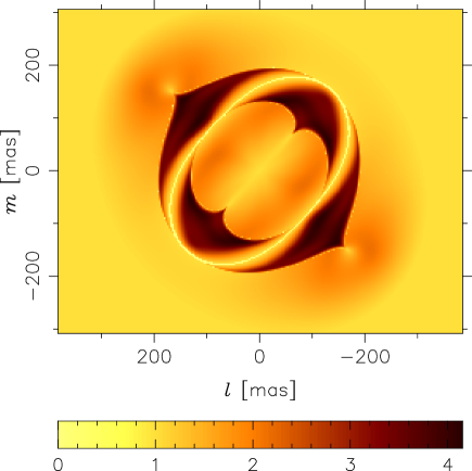
Figure 1: Bias factor in the KNE LensClean variant. This factor is proportional to the residual reduction from Eq. (10) in one LensClean iteration for a constant surface brightness source. The lens model assumed for this plot is very similar to the best model for B0218+357.

We tried different methods of improving LensClean in this respect, the most successful one we want to present here. The simple idea is to apply an adaptive loop gain depending on source position and lens model. This is applied as a factor to $\Delta$ instead of $S$. To obtain a unique recipe and keep things simple, we demand that this factor does not depend on the observed brightness distribution. We can then assume an arbitrary brightness distribution to calculate the optimal correction factor and use the constant surface brightness scenario for this. The correction factor is then simply the inverse bias factor we would get from Eq. (10) in this case (see also Fig. 1):

$$\Delta^{\prime} =g\,\frac{\sum\limits_{kk^{\prime}}\mu_{k}\mu_{k^{\prime}}B_{kk^{\prime}}}{\Bigl{(}\sum\limits_{k}\mu_{k}\Bigr{)}^{2}}\,\Delta$$ (11)

$$=g\left(\frac{\sum\limits_{k}\mu_{k}I_{k}}{\sum\limits_{k}\mu_{k}}\right)^{2}\quad\text{.}$$ (12)

We included a factor $g$ here which plays the role of a loop gain scaling factor and in the case of no lens is the same as $\gamma\,(2-\gamma)$ and therefore monotonically related to the conventional loop gain $\gamma$ for $0\leq\gamma\leq 1$. We now select the source position for the next iteration by searching the maximum of $\Delta^{\prime}$. The flux density which should be subtracted at this position to achieve exactly this decrease in $R^{2}$ can easily be calculated by going back to Eq. (6) and solve for the new $S^{\prime}$ with the known $\Delta^{\prime}$.

$$S^{\prime}=\left(1-\sqrt{1-g\,\frac{\sum\limits_{kk^{\prime}}\mu_{k}\mu_{k^{\prime}}B_{kk^{\prime}}}{\Bigl{(}\sum\limits_{k}\mu_{k}\Bigr{)}^{2}}}\right)\,S$$ (13)

This expression can be interpreted more easily in the limiting case of a small gain $g$:

$$S^{\prime}\approx\frac{g}{2}\,\frac{\sum\limits_{k}\mu_{k}I_{k}}{\left(\sum\limits_{k}\mu_{k}\right)^{2}}$$ (14)

This is proportional to a mean of the source plane fluxes $I_{k}/\mu_{k}$, estimated from the individual images, weighted with $\mu_{k}^{2}$ and scaled with $g/2$. The remaining scaling factor is responsible for compensating the bias.

Since in B0218+357 we have not only a relatively well resolved ring but also the two strong compact components, we have to assure that the modified method also works in this case. For images with equal magnification, the adaptive loop gain corrects for the bias caused by the number of images, which is sensible. Numerical tests show that the adaptive gain works very well for compact and extended emission and minimizes the bias effects. Due to the different definition, higher values can be used for $g$ than for $\gamma$ without deteriorating the results. For equal magnifications of $n$ well separated images, both methods are equivalent if

$$g=n\,\gamma\,(2-\gamma)$$ (15)

is used.

Please note that the selection rule of LensClean components does not influence the results in the idealized case where the Clean iterations are performed until convergence is reached. For practical work, however, convergence of (Lens)Clean is so slow at later stages that the unbiased LensClean variant actually does improve the results considerably even if a few 1000 iterations are done. The real differences caused by different lens models are so small that any bias effects have to be avoided by all means. We therefore used our unbiased LensClean variant for all the calculations presented here.

The more uniform Cleaning with the unbiased algorithm does also accelerate convergence for good lens models by an order of magnitude while it does not influence the residuals in other cases very much. It therefore improves the ability of the residuals to discriminate between good and bad lens models after a moderate number of iterations.

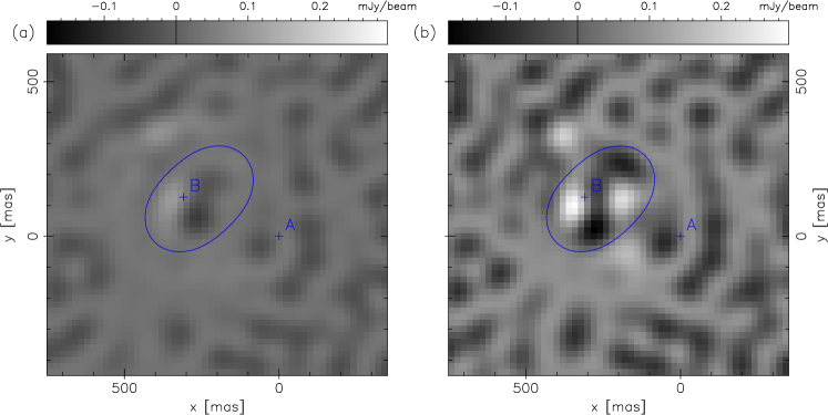
Figure 2: Uniformly weighted image plane residuals for a simulated data set using the known lens model parameters. The top panels (a+b) show the results after 2000, the bottom panels (c+d) after 100 000 iterations (with a very different grey scale; the total range shown is a factor of $\sim 5$ smaller). The unbiased variant is on the left (a+c), the KNE variant on the right (b+d). For 2000 iterations the unbiased version of LensClean is clearly superior while both are more or less equivalent in the limit of very many iterations. The expected noise of the dirty maps is 0.14 mJy per beam. The critical curve and the two bright images are marked.

In Fig. 2 we compare image plane residuals for both variants of LensClean. For these maps we used a simulated data set which was made using the best fitting lens and source model for B0218+357. After building the $uv$ data set with the same $uv$ coverage as in the real data set, we added noise and performed self-calibration with the known emission model. This last step is necessary to be able to compare the results with LensClean runs for the real data set which will be presented in Paper II. We see that for a moderate number of 2000 iterations, which is quite typical for real model fitting runs, the residuals are significantly higher for the KNE variant than for the new unbiased version. The alignment of the residuals with the critical curve of the lens could in such a case be misinterpreted as a bad fit of the lens model. Only if many more iterations are performed do the residuals become similar.

Note that the image space residuals become much smaller than the expected rms noise in the dirty map. This is well known from unlensed Clean where the residuals, by including the noise in the emission model, can be reduced without limit. In the lensed case, the situation is more complicated because in the multiply imaged regions the Cleaning is constrained by lens model. If these regions are of comparable size to the resolution of the observations (or even smaller), the residuals can still be reduced significantly below the noise level, especially in combination with self-calibration (see below).

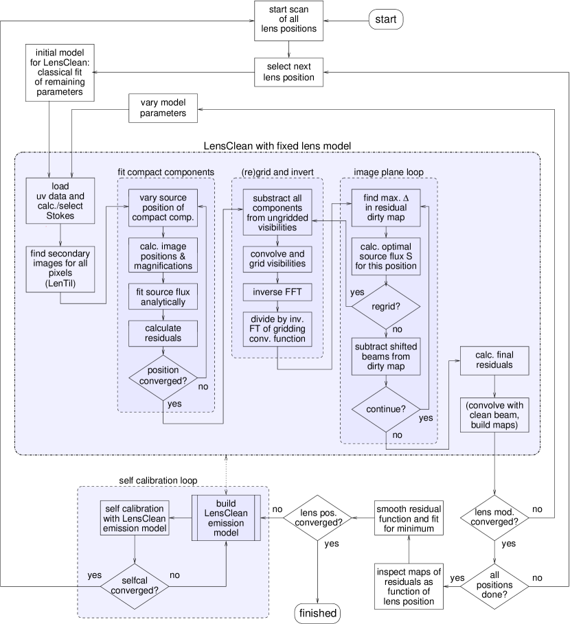
Figure 3: Schematic flow-chart of the complete LensClean algorithm as we used it for fitting lens models for B0218+357. Most important is the inner core (large shaded box) which builds an emission model and calculates the residuals for a given fixed lens model. If required, maps of the lens and source plane are also produced. Built around this core is an algorithm to determine the optimal lens model, including a loop for the self-calibration of the data. Inside of the self-calibration loop the same LensClean core is used to build an emission model.

4.3 Details of the inner core

Figure 3 illustrates the structure of our implementation of the inner LensClean core in the large shaded box. In detail it works like this. Before any Cleaning is done, we calculate for each pixel (‘primary image’) in our image plane map area the corresponding source position and the positions of all other ‘secondary images’ which are produced for the same source position by the lens. Finding all images for a given source position for a SIEP lens model implies solving a quartic equation. The one already known primary image can be divided out, leaving a cubic equation to solve. This can and should be done analytically with special care to avoid any errors in this step. Incorrect image positions for even one pixel in the map will make the residuals after Cleaning unusable and hence make model fitting impossible. Errors for individual pixels will often allow more freedom for the Cleaning process and thus reduce the residuals. The outer loop of lens model fitting will happily stick at such models, leading to wrong results.

When all images are found, the magnifications are calculated. Sometimes it happens that a few pixels have very high magnifications of the order of a few hundred. These can change the LensClean residuals considerably which increases the numerical noise of the residual function. With artificial data we established that the fits improved when such pixels (including their secondary images) were excluded from LensCleaning without introducing systematic errors.

For each iteration, the optimal source position (on the regular grid required by the FFT) and flux density is found with the unbiased LensClean method described above. Scaled dirty beams are then subtracted in image space for each image position. For the secondary images, which are not located at exact grid positions, we distribute the flux over the four nearest pixels in a way which is equivalent to bilinear interpolation. This is essential to avoid large discontinuities in the residual function which would fool the outer residual minimization with local minima. Errors of the image space representation are minimized by using a truncated Gaussian multiplied by a sinc-function as gridding convolution function and by using small pixels. Aliasing is only noticeable in the first few Clean iterations when the subtracted flux density is still high. After a number of iterations of this kind, all accumulated LensClean components are subtracted at their exact positions from the ungridded visibilities which are then regridded to get a new residual map with gridding errors of all iterations up to then removed. This is known as Cotton-Schwab algorithm in unlensed Clean  (Schwab, 1984; Cornwell et al., 1999) but is much more important in LensClean because of the secondary images which are not located exactly on the grid. Working directly on the $uv$ space visibilities would be desirable but is computationally prohibitively expensive because it would imply inversion of the FT in each iteration for many image (or source) positions in order not to miss the optimal position.

Because of the dominance of the bright components, it is essential to keep any errors caused by these as small as possible. These residual errors would otherwise hide any effects of the ring which are essential to obtain constraints for the galaxy position. To avoid errors caused by the discrete nature of the pixels for the bright images, we remove them partially before the normal iteration starts. This is done by one ungridded LensClean iteration (model fitting with a free continuous source position and flux and subtraction of the best fit afterwards) at the beginning with a loop gain of nearly unity so that the compact image is removed without affecting the smooth background of the ring. The ring itself will influence this first ungridded step to some degree, which might produce bias effects in later stages. Tests with artificial data showed, however, that these biases are too small to affect the results seriously. Small errors in the positions of the bright components will be corrected for in the later iterations anyway.

We did not enforce zero flux outside of user-selected windows because tests with simulated data showed that this can introduce serious systematic shifts of the residual minimum.

4.4 Non-negativity constraints

To reduce the freedom of the models without excluding physically realistic models, a non-negativity constraint for the flux components would be desirable. In the lensed case, combinations of positive and negative components in regions of rapidly varying magnifications close to the caustics can produce image plane brightness distributions which could not be reproduced by only positive components with the same lens model. They therefore reduce the residuals for incorrect lens models without changing them much for the best lens model. With a non-negativity enforcing algorithm the accuracy of the lens model could therefore improve considerably.

Well known approaches in Clean, like allowing only positive components, stopping at the first negative component or deleting negative components afterwards, are not able to find the best non-negative solutions because negative components occuring during later stages of Clean are often only needed to compensate for overestimated positive components in earlier iterations. This happens especially if the weighting of the data is changed between Clean iterations. Disregarding these compensating components prevents Clean from finding an optimal solution. Other methods like the NNLS algorithm are able to derive a true optimal non-negative solution in the unlensed case. In principle, NNLS can be extended for a lensed scenario in a straight-forward way. Unfortunately, the numerical difficulties are much more serious than in the unlensed case.

We recently found an alternative solution by modifying Clean to include a non-negativity constraint in a strict way. It works by allowing negative components only at positions where positive ones have been put before and only with absolute fluxes smaller than the total combined flux at this position up to that iteration. In this way negative components are allowed to modify earlier positive ones, but negative total fluxes can never occur. This new method is not implemented in standard software packages like AIPS or DIFMAP but is now part of our own code. Tests have shown that it can improve the solution in the unlensed case significantly, especially if the emission model is to be used for self-calibration. In the latter case, the well-known negative features resulting from incorrect calibration can not be included in the emission model so that they are removed later with self-calibration, at least if there are large regions without emission in the map area so that the non-negativity constraint can become active at all.

In the lensed scenario, the flux density from Eq. (9) or (13) is used directly only if it is either positive itself or if at least the sum with the already existing components at the same position is not negative. Otherwise the absolute value of a negative $S$ is decreased until the sum of components at this position exactly vanishes. This procedure is followed for all pixel positions and the resulting potential decrease of residuals $\Delta$ is calculated from Eq. (6) with the modified value for the source flux $S$. In the same way as without the non-negativity constraint, the pixel with maximal $\Delta$ is then selected in this iteration.

Experiments with this variant of LensClean showed that it does indeed reduce the unwanted freedom of models but does on the other hand introduce discontinuities and bias effects in the residual function. These are much weaker than with the more standard methods of rejecting negative components, but they are still significant. Because these effects have to be avoided in any case, we generally did not exclude negative components. The only exception is the brightness model used for self-calibration (see below). But even here the inclusion of negative components would not have changed the results noticeably.

The reason for the current failure of non-negativity enforcing versions of LensClean probably lies in the fact that total negative components are often necessary to compensate for small errors originating from other effects, e.g. the gridding of the model. These errors can change with variations of the lens model so that the increase of residuals caused by not allowing negative components produces lens model dependent bias effects. A better understanding of these effects is highly demanded and it is our hope that a better algorithm including the non-negativity constraint without introducing other problems can be developed in the future.

4.5 The outer loop: Fitting the lens model

After LensClean found the best source brightness model for a given set of lens model parameters, the residuals from the inner loop are used to find the best lens model in the outer loop (see Fig. 3 for an illustration).

Even with all the precautions discussed before, the residuals are no absolutely smooth function of the lens model parameters, making it difficult to fit the lens model. We use the downhill simplex method (cf. Press et al., 1992) because more sophisticated minimization methods which rely on smooth quadratic minima did not prove to be superior in this case. Simultaneous LensClean fits of all five free parameters are dangerous in our case; they often get stuck at local minima. This is a result of the very different magnitude of the eigenvalues of the matrix describing the residual function near its minimum. Three of the lens model parameters could be fitted with the very bright compact images alone, leading to three very high eigenvalues. For the remaining two, the position and structure of the much weaker and less compact structures in the ring have to be used, causing two much smaller eigenvalues. This combination of very high sensitivity in certain directions with very low sensitivity in other directions is a highly problematic case for any minimization method. Finding the global minimum of a long, narrow and bent valley is never easy, especially if numerical noise (not to be confused with the noise of the observations) causes additional fluctuations.

To be absolutely sure to find a global minimum in the allowed parameter range, we scan all realistic values of the lens position $\mn@boldsymbol{z}_{0}$ and fit only the remaining three model parameters (lens mass scale $\alpha_{0}$ and ellipticity $\varepsilon_{x}$ and $\varepsilon_{y}$) for each fixed $\mn@boldsymbol{z}_{0}$. A number of three parameters could be fitted with the information from the two strong components alone with very high accuracy. We therefore avoid using the low eigenvalues provided by the ring for the minimization of residuals and achieve a highly improved stability. The ring still shows its effects in the best residuals as a function of $\mn@boldsymbol{z}_{0}$, of course. To assist the LensClean model fitting, we start with a classical lens model fit for each $\mn@boldsymbol{z}_{0}$ which is already very close to the final model. The combined scanning/fitting approach is nevertheless numerically very expensive and at the limit of what can be done with a cluster of modern PCs or workstations. It does on the other hand allow the estimation of confidence regions from the maps of residuals as function of $\mn@boldsymbol{z}_{0}$ and provides an invaluable diagnostic to detect possible numerical problems. Only if the algorithm works optimally, do the residuals show a smooth quadratic minimum. To reduce the remaining numerical noise, smooth polynomial functions are fitted to the residual function $R^{2}(\mn@boldsymbol{z}_{0})$ to determine the minimum and confidence regions. A similar fit for the remaining lens model parameters evaluated at the residual minimum provides the final optimal lens model.

We also tried to separate the effect of the two compact components from the effect of the ring. One attempt was to fit the other parameters for given $\mn@boldsymbol{z}_{0}$ classically and use LensClean only to calculate the final residuals for this model. This method, if successful, would accelerate the complete model fitting by a factor of $\sim 100$. Unfortunately the residuals from the two compact components are so strong, although we tried to remove their influence by several methods, that they lead to serious systematic errors in the final results. These approaches were therefore not used to produce the results presented in Paper II.

In order to correct for possible changes of the flux ratio A$/$B caused by variability in combination with the time-delay or by propagation effects, we also fit lens models to modified data sets where we either added or subtracted flux at the position of one of the components to compensate for the effect. Another approach is to artificially change the amplification of the lens model by some amount in a small region around one of the bright images. We found that both methods lead to very similar results. The effect on the best lens models in the case of B0218+357 will be discuss in Paper II.

4.6 Self-calibration

We started our LensClean algorithm with a calibrated data set which was first used to make a map with unlensed Clean and used the self-calibration from this procedure. After finding a best fitting lens and source model for the given data, we used this model (now with positivity of components enforced) to self-calibrate the data set. It is important that the same weighting is used for the self-calibration as for the LensClean model fitting. For uniform weighting, the data set was re-weighted to be able to use DIFMAP for the self-calibration. A moderate number of alternating LensClean runs and self-calibration steps where used for the (fixed) lens model. We then started with these recalibrated data from the beginning (see Fig. 3). It showed that only a few iterations of LensClean lens model fitting and self-calibration were necessary to get a stable result.

In the self-calibration we allowed independent phase and magnitude changes for each 1 min integration. This may introduce too much freedom but has the advantage that (if the same procedure is applied to artificial data sets) the real and simulated data are guaranteed to have the same level of calibration so that results of the two can be compared with confidence.

In order to test the robustness of the procedure we also started with very badly calibrated data and with self-calibrating with an incorrect lens model. After a few iterations the fits always converged to the same best solution which established the stability of this method.

It is not possible to use self-calibration as part of the innermost LensClean loop as it is often done with Clean, because the comparison of residuals of different self-calibrations introduces an extreme level of numerical noise which completely hides the effects of different lens models. The method would also be numerically too expensive to be applied on a regular basis. The extensive numerical tests with real and simulated data proved that using self-calibration only after an optimal lens model is found is sufficient to remove any initial calibration errors and to find the best solution.

4.7 Goodness of fit, error statistics

Several stopping criteria for the LensClean iteration have been discussed by Kochanek & Narayan (1992). We decided to use the simple scheme of taking a fixed number of iterations (about 500 to 5000), using the remaining residuals $R^{2}$ as a direct measure for the goodness of the fit. In the outer loop, the lens model parameters are then varied to find a minimum of $R^{2}$. We decided to use the $uv$ space residuals $R^{2}$ instead of other measures for the residuals for the outer loop in order to get a consistent solution for the lens model and source structure. When computing residuals in $uv$ space, we also avoid the problem of correlated errors in image space.

Different weighting schemes were tested with artificial data sets with the result that the high sensitivity for small scale structures provided by uniform weighting helps in getting useful constraints for the models in the initial stages of self-calibration. Interpretation of the residuals is simpler for natural weighting of course, because in this case $R^{2}$ is equal to $\chi^{2}$ and the complete algorithm is equivalent to a maximum likelihood fit of the lens mass model and source brightness distribution.

For real statistical weights of $1/\sigma_{j}^{2}$ and applied weights $w_{j}$, the expected value of $R^{2}$ for the correct lens and emission model is

$$<R^{2}>=\sum_{j}w_{j}\sigma_{j}^{2}$$ (16)

and the standard deviation

$$\sigma_{R^{2}}=\sqrt{2\sum_{j}w_{j}^{2}\sigma_{j}^{4}}\quad\text{.}$$ (17)

Usually the effective number of parameters of the emission model (estimated by the number of non-overlapping beams in the map area) is much smaller than the number of visibilities so that the implicit fit of the emission model does not change the error statistics significantly. The residuals will be reduced by some amount, but this reduction is (almost) the same for all lens models and does not influence the fit of the lens model. The only concern could be that the effective number of emission model parameters changes with the lens model via changes of the area of doubly and quadruply imaged regions, in which the emission model has less freedom than in singly imaged regions. The effect of this has been estimated with artificial data consisting of only noise. Differences of the residuals for different lens models are a direct measurement of this possible bias. From these simulations we learned that the shift of the best lens model originating from this effect is much smaller than the statistical errors and can thus be neglected in the following.

We now assume that the emission model has been fitted for each lens model and discuss the residuals without worrying about the emission models. The best fitting lens model will have residuals which are smaller than the expectation from Eq. (16) by $\Delta R^{2}$ (it has by definition the smallest residuals of all models). If the number of fitted parameters is much smaller than the number of visibilities, $\Delta R^{2}\ll R^{2}$ and the residuals can be used directly to judge the goodness of fit. For $\chi^{2}$ statistics (natural weighting: $w_{j}=1/\sigma_{j}^{2}$), mean and standard deviation of the residual minimum are $\nu$ and $\sqrt{2\nu}$, respectively, where the number of degrees of freedom $\nu$ is the difference of the number of visibilities (real and imaginary part counted separately) and the number of fitted parameters. The difference $\Delta\chi^{2}$ also follows a $\chi^{2}$ distribution with $\nu$ given by the numbers of fitted parameters and can be used to determine confidence limits. For non-natural weighting schemes, this simple interpretation is not possible. In this case $\nu$ does not only depend on the weights and the numbers of visibilities and parameters but also on the model and the data themselves. We then can still use the best $R^{2}$ to judge if our fit is acceptable but we cannot use differences $\Delta R^{2}$ to the best $R^{2}$ to determine confidence limits in the rigorous way in which it is possible for natural weighting from the $\chi^{2}$ distribution.

In Wucknitz (2002) we presented an analytical approximation which makes it possible to estimate confidence regions also for general weighting. The result applied to our case says that the difference of the residuals for the best fitting and true model is expected to be

$$\left<\Delta R^{2}\right>\approx\frac{\sum_{j}w_{j}^{2}\sigma_{j}^{2}}{W}$$ (18)

for one (lens-)model parameter. By analogy to natural weighting where this value becomes unity, we scale this residual difference with the normal limits from the $\chi^{2}$ distribution to obtain different confidence limits for an arbitrary number of parameters.

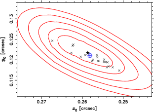
Figure 4: Results of Monte Carlo simulations for the 15 GHz VLA data (Stokes I) showing residuals as a function of lens position. We picked one of the runs with a minimum (star) close to the model used to build the data (crosshair) for the contour plot (confidence limits of 1, 2, 3, 4, 5$\cdot\sigma$). The other Monte Carlo results are shown as crosses.

To detect possible systematical errors and to check the accuracy of the confidence limit estimates for uniform weighting, we performed a small number (21) of Monte Carlo simulations. Even though we did not include self-calibration to save computing time, a total of about two years of CPU time on modern PCs was needed for these simulations. We took a model for the lens and brightness of the source from earlier stages of our LensClean fits of the B0218+357 data to produce an artificial data set and used the same algorithm (without self-calibration) as for the real data with uniform weighting. The source model does not reproduce the real data exactly so the results are not meant to be compared with the results of the real fits. The idea is instead to compare the distribution of residual minima with the expectations from the residual differences and error statistics. The results in Fig. 4 show that the agreement is indeed quite good, although the simulated distribution seems to be somewhat flatter than the approximated estimate. Of the 21 runs a number of 17 (81 per cent) is within the expected $1\,\sigma$ region and all are within $2\,\sigma$. Since error statistics expects only 68 per cent inside the $1\,\sigma$ region we conclude that our error estimates are at least not excessively overoptimistic.

Despite the cautionary note above, the size of the simulated confidence regions is also very similar to the real data results which are presented in Paper II.

5 Non-isothermal models: LenTil

We explained before that LensClean relies on a very robust method to solve the lens equation i.e. to find all images for a given source position. Because of this we have done most of our work with isothermal elliptical potentials for which this can be done analytically. To be able to use more general lens models with LensClean, we developed a new algorithm which can invert the lens equation for any lens model for which the deflection angle can be calculated as a continuous function of the image position (with the possible exception of known singularities).

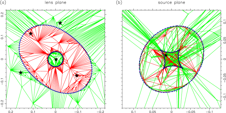
Figure 5: Image search with the LenTil algorithm. In addition to the initial tiling, this plot includes the subtilings performed in the search of images for one source position. (a) Lens plane with critical curves and five images (stars), (b) source plane with caustics and source position (star).

Our algorithm (called LenTil for ‘lens tiling’) is based on ideas similar to those used by Keeton (2001a, b) in his software package. LenTil is adapted especially for the use with LensClean which means it has to be extremely reliable (failure in less than one of $10^{8}$ cases) while still being sufficiently fast to be able to invert the lens equations for all pixels without increasing the already high computational demands of LensClean too much. LenTil is used for very many source positions for each lens model so some overhead can be accepted to prepare the calculations for each model. Including this overhead, the total time for one inversion is of the order a few milli-seconds.

The basic idea is the following. The lens plane is subdivided in a large number of triangular tiles which are then mapped to the source plane with the given lens model. There it can be tested in which of the source plane tiles the source position is located. Other tiling methods would then use the lens plane position of these tiles to start standard numerical root finding algorithms from there. This approach is well suited for standard lens modelling where the failure in a few cases does little harm but this is not acceptable for LensClean. Our algorithm therefore uses the tiles in which the source is located to start a subsequent subdivision until the required accuracy is reached. During this subdivision the source will often leave the initial tile and be located in a neighbouring tile after a subdivision step. In these cases the subdivision process continues with these new tiles. Special care is needed to assure convergence of the subdivision process in all cases. Sometimes the subtiles become degenerate which has to be avoided because it prevents convergence. The tests of whether or not the source is located within a tile have to be done in a special way to lead always to consistent results even if the source is located exactly (in a numerical sense) on one of the bordering edges of a tile. This is difficult when the source lies not only on one of the edges but exactly on one of the vertices (i.e. on at least two edges). These possible problems have to be detected and must in bad cases be corrected by shifting the source by a very small amount slightly above the numerical resolution but far below the required accuracy, and restarting the algorithm.

In the preparation phase, which has to be performed once for each lens model, the initial tiling is built. In this phase it is extremely important to detect all critical curves which separate regions of different parities because these regions have to be treated separately in the later subdivision stages. Critical curves have to be sampled sufficiently densely to avoid loosing very close multiple images with a high magnification. Some special care is also needed to treat different kinds of singularities of lens models (pointmass-like ones with diverging and SIS-like ones with finite deflection angles) correctly.

We start by covering the area of interest with one very large triangular tile. We then divide this initial tile by adding new vertices very close to all the (known) singularities of the lens model. In the models used with LensClean so far, we only had one singularity per model. From the kind of singularity we infer the number of critical curves that should enclose it. After searching for the critical points on a straight line drawn from the singularity outwards, we put new vertices in all the domains of different parities. Then we subdivide the tiles until their sides are all below a preselected limit and until the critical lines and ‘cuts’ are sampled sufficiently densely.

In all these and the following subdivisions we always take care that no side of a tile ever crosses a critical curve, i.e. that no side connects regions of different parity, by introducing additional vertices at such crossing. This is important to assure that the tiles do (in the limit of infinite subdivision) project to the source plane with a well defined parity. Otherwise it could happen that some regions of the source plane are missed or others are sampled several times. This would result in missing images or additional phantom images. Both have to be avoided.

Figure 5 shows a typical tiling in the lens and source plane with five images found by the subsequent subdivision. After an extensive testing phase, the LenTil algorithm is now in a state in which it can be used for LensClean. Depending on the lens models, it can still double the CPU time needed compared to LensClean with the analytical SIEP inversion but this is regarded as acceptable.

The LenTil code is refined continuously and it is therefore premature to make it publically available. More details of the implementation can be found in Wucknitz (2002).

6 Source reconstruction

Although the pointlike Clean components are an optimal representation of the data in the sense of a maximum likelihood model, they usually represent the true source maps very badly because they contain signals with very high spatial frequencies which are not measured directly because of the limited $uv$ range of the observations. These high frequency parts are highly uncertain and should therefore be reduced to produce the final maps. The standard regularisation method with Clean is to convolve the collection of components with a Gaussian ‘Clean beam’ whose size is chosen in a way to resemble the dirty beam in its central parts. This is a sensible approach although it has its shortcomings and there is no rigorous mathematical foundation for it. In practice the standard Clean beam convolution is used on a regular basis and leads to satisfying results. We therefore want use the same idea generalized to the lensed situation to produce source plane maps with LensClean.

The approach presented by Kochanek & Narayan (1992) uses circular beams and chooses the size so that they just cover the intersection of the projected single image beams of all corresponding images. With this approach the combined beam is in each direction larger or equal to the smallest of the single beams and does not introduce spurious small scale features. This procedure has its justification for equal magnifications, but becomes very inaccurate for high magnification ratios. In this case the projected beams should be weighted in some way according to the lens plane flux densities which are proportional to the magnifications of the images. Images with very low magnification should contribute less to the final beam than images with a high magnification.

Before we can translate the concept of a beam to the source plane, we have to understand its meaning in the lens plane in the context of the linear least squares problem which is solved by standard Clean. We formulate the problem in an algebraic way which can then be extended easily. The general problem of this kind can be written like this:

$$\mn@boldsymbol{y}={\textbf{{A}}}\,\mn@boldsymbol{x}+\text{noise}$$ (19)

Here $\mn@boldsymbol{x}$ denotes the vector of model parameters (brightness distribution in our case), $\mn@boldsymbol{y}$ is a vector describing observations (visibilities in our case) and the linear function connecting the two is written as a matrix A (the Fourier transform here). This equation is the general version of Eq. (1) but the brightness distribution $I(\mn@boldsymbol{z})$ is written as a discrete vector $\mn@boldsymbol{x}$ and the visibilities $\tilde{I}_{j}$ as vector $\mn@boldsymbol{y}$. With a weighting matrix W, the residuals for observations $\mn@boldsymbol{y}$ and model $\mn@boldsymbol{x}$ are

$$R^{2}={(\mn@boldsymbol{y}-{\textbf{{A}}}\mn@boldsymbol{x})}^{\dagger}\,{\textbf{{W}}}\,(\mn@boldsymbol{y}-{\textbf{{A}}}\mn@boldsymbol{x})\quad\text{.}$$ (20)

In our case the matrix W consists only of the visibility weights as diagonal elements. The residuals are minimal if the derivative with respect to $\mn@boldsymbol{x}$ vanishes, which leads to the equation

$${\textbf{{B}}}\,\mn@boldsymbol{x}=\mn@boldsymbol{I}_{\mathrm{D}}\quad\text{,}$$ (21)

where B denotes the matrix of the dirty beam $({\textbf{{B}}})_{jk}=B(x_{j}-x_{k})$ and $\mn@boldsymbol{I}_{\mathrm{D}}$ the vector of the dirty map $(\mn@boldsymbol{I}_{\mathrm{D}})_{j}=I_{\mathrm{D}}(x_{j})$:

B $$=\frac{1}{W}{{\textbf{{A}}}}^{\dagger}{\textbf{{W}}}{\textbf{{A}}}$$ (22)

$$\mn@boldsymbol{I}_{\mathrm{D}} =\frac{1}{W}{{\textbf{{A}}}}^{\dagger}{\textbf{{W}}}\,\mn@boldsymbol{y}$$ (23)

The normalization with $W=\operatorname{Tr\,}{\textbf{{W}}}$ is used by convention but is not necessary. In this way the dirty map resembles physical units and the dirty beam has a central value of unity.

If a lens is introduced in the problem, we can write the brightness distribution in the lens plane as a linear function of the brightness distribution of the source plane:

$$\mn@boldsymbol{x}={\textbf{{L}}}\,\mn@boldsymbol{x}_{\mathrm{s}}$$ (24)

The matrix L describes the lens effect. If the vectors $\mn@boldsymbol{x}$ and $\mn@boldsymbol{x}_{\mathrm{s}}$ are used to describe a collection of $\delta$ components, $L_{kk_{\mathrm{s}}}$ is the magnification of the image $\mn@boldsymbol{z}_{k}$ if it is mapped to the source position ${\mn@boldsymbol{z}_{\mathrm{s}}}_{k_{\mathrm{s}}}$ and 0 otherwise. Of course the representation of $\mn@boldsymbol{x}$ and $\mn@boldsymbol{x}_{\mathrm{s}}$ has to be complete, i.e. each component of $\mn@boldsymbol{x}$ must correspond to one component of $\mn@boldsymbol{x}_{\mathrm{s}}$ and each component of $\mn@boldsymbol{x}_{\mathrm{s}}$ must correspond to one or more images in $\mn@boldsymbol{x}$. Writing Eq. (19) with $\mn@boldsymbol{x}_{\mathrm{s}}$ instead of $\mn@boldsymbol{x}$, we see that the effect of the lens is to replace the matrix A by a modified matrix ${\textbf{{A}}}_{\mathrm{s}}={\textbf{{A}}}{\textbf{{L}}}$. The ‘source plane dirty beam’ can then be defined as

$${\textbf{{B}}}_{\mathrm{s}}={{\textbf{{L}}}}^{\dagger}{\textbf{{B}}}{\textbf{{L}}}$$ (25)

analogous to the lens plane dirty beam in Eq. (22). This source plane dirty beam has, however, not the same properties as B. Whilst B is translation invariant so that Eq. (21) can be read as a convolution, this is not true for ${\textbf{{B}}}_{\mathrm{s}}$ in the general case. Explicitly, the source plane dirty beam can be calculated using the definition of L:

$$B_{\mathrm{s}}(\mn@boldsymbol{z}_{\mathrm{s}},\mn@boldsymbol{z}^{\prime}_{\mathrm{s}})=\sum_{\begin{subarray}{c}\mn@boldsymbol{z}(\mn@boldsymbol{z}_{\mathrm{s}})\\ \mn@boldsymbol{z}^{\prime}(\mn@boldsymbol{z}^{\prime}_{\mathrm{s}})\end{subarray}}\mu(\mn@boldsymbol{z})\mu(\mn@boldsymbol{z}^{\prime})B(\mn@boldsymbol{z},\mn@boldsymbol{z}^{\prime})$$ (26)

In this sum $\mn@boldsymbol{z}$ and $\mn@boldsymbol{z}^{\prime}$ run over all images of the source components $\mn@boldsymbol{z}_{\mathrm{s}}$ and $\mn@boldsymbol{z}^{\prime}_{\mathrm{s}}$, respectively. For our first attempts to produce a map of the source plane of B0218+357, which will be presented in Paper II, we introduce some approximations. We assume that the images are well separated, i.e. that their respecting dirty beams do not overlap (only the diagonal elements of the sum in Eq. (26) contribute) and that the magnification close to the individual images is not varying significantly over an area corresponding to the beam. With these approximations it is possible to express distances in the lens plane $\Delta\mn@boldsymbol{z}$ by the corresponding distance in the source plane $\Delta\mn@boldsymbol{z}_{\mathrm{s}}$ using the local magnification matrix M:

$$B_{\mathrm{s}}(\Delta\mn@boldsymbol{z}_{\mathrm{s}})=\sum_{k}\mu_{k}^{2}\,B({\textbf{{M}}}_{k}\Delta\mn@boldsymbol{z}_{\mathrm{s}})$$ (27)

The index $k$ runs over all images for the given source position. For small $\Delta\mn@boldsymbol{z}_{\mathrm{s}}$ this source plane beam is approximately translation invariant but it depends on the source position on larger scales.

Now we use the standard approximation of a Gaussian for the lens plane dirty beam and write

$$B(\Delta\mn@boldsymbol{z})={\mathrm{e}}^{-{\mn@boldsymbol{z}}^{\dagger}{\textbf{{G}}}\mn@boldsymbol{z}/2}\quad\text{.}$$ (28)

The matrix G determines the parameters of the Gaussian and can be calculated from the major and minor axis FWHM $a$ and $b$ and position angle $\phi$ of the beam. The same parametrization as discussed in a different context in Appendix LABEL:II-sec:app_shapes of Paper II can be used here. If the parameters are used as defined before, the beam matrix is ${\textbf{{G}}}=(8\ln 2)\,{\textbf{{E}}}^{-1}$. With the properties of the Fourier transform it is easy to show that G is proportional to the second moment matrix of the $uv$ coordinates and can thus be calculated easily.

Now we can fit an effective total Gaussian to the central part of the source plane beam from Eq. (27). This is done by expanding the exponential in Eq. (28) to first order and write the sum again as exponential for which it is the first order Taylor expansion. The resulting beam is again a Gaussian, now with central value $\sum\mu_{k}^{2}$ and with parameter matrix

$${\textbf{{G}}}_{\mathrm{s}}=\frac{\sum\limits_{k}\mu_{k}^{2}\,{\textbf{{M}}}_{k}{\textbf{{G}}}{\textbf{{M}}}_{k}}{\sum\limits_{k}\mu_{k}^{2}}\quad\text{.}$$ (29)

This is a weighted mean of the individual backprojected matrices ${\textbf{{M}}}_{k}{\textbf{{G}}}{\textbf{{M}}}_{k}$. For very different individual source plane beams (i.e. for very different magnifications) the combined beam is dominated by the smallest individual beam which has the highest magnification. This means that the effective source plane resolution can be improved beyond the lens plane resolution by the lens.

Beams in standard Clean are normalized to have a central value of unity. This leads to maps in physical units per beam (e.g. $\mathrm{Jy}/\mathrm{beam}$). For resolved sources this can be transformed to units of surface brightness (e.g. $\mathrm{Jy}/\mathrm{arcsec}^{2}$) easily. In our case, the beams are not constant but depend on the position in the source plane. If the same normalization would be used in this case, the resulting map would have varying units over the field and would not conserve total flux. Even for well resolved sources with constant surface brightness, the values of the map would depend on the position which is clearly not desirable. We therefore normalize the beam to have not a constant central value but a constant total flux of unity. This leads to maps in units of surface brightness and preserves total flux. The final source plane beam is then

$$B_{\mathrm{s}}(\Delta\mn@boldsymbol{z}_{\mathrm{s}})=\frac{\sqrt{\lvert{\textbf{{G}}}_{\mathrm{s}}\rvert}}{2\pi}{\mathrm{e}}^{-{\mn@boldsymbol{z}_{\mathrm{s}}}^{\dagger}{\textbf{{G}}}_{\mathrm{s}}\mn@boldsymbol{z}_{\mathrm{s}}/2}\quad\text{.}$$ (30)

The source plane reconstruction with a beam following Eq. (29) and (30) is certainly not optimal. The approximations used do not work very close to caustics and the whole procedure is somewhat arbitrary. On the other hand it is based directly on the standard Clean beam convolution which is known to work well. Any more optimal method will probably be an integral part (in the sense of regularisation) of the algorithm and not be applied at the end once the best brightness model is known. Investigations of better approaches could therefore start with the simpler unlensed problem and be generalized from that.

It is now possible to use the reconstructed source plane beams and map them back to the image plane to produce a superresolved image plane map of the lens system. In singly imaged regions, this superresolved map is equal to a normal Clean map because projecting the beam forth and back does not change it. It is only the combination of several beams in multiply imaged regions which provides the opportunity to improve the resolution in the lens plane map.

In Paper II we show reconstructed maps of the unlensed source of B0218+357 on different scales as well as standard and superresolved lens plane maps.

7 Discussion

Multiple images of lensed extended sources do potentially provide far better constraints for lens mass models than simple multiply imaged point sources because they probe the lensing potential not only at a small number of discrete positions but over wide areas of the lens plane. In order to utilize these constraints, it is necessary to fit not only for the mass model of the lens but also (implicitly or explicitly) for the brightness distribution of the source. This makes the model fitting for extended sources much more difficult than for compact sources which can be described by a position and flux density alone. We showed how the task can be performed using an improved version of the LensClean algorithm. In an inner loop, the brightness model of the source is optimized for a given lens model, while an outer loop uses the residuals from the inner loop in order to determine the optimal lens model parameters.

As a test case we used the lens B0218+357 where the beautiful Einstein ring shown by radio observations potentially provides constraints to determine the position of the lens with sufficient accuracy. Surprisingly, variants of LensClean have been used only for very few cases before. This is partly a result of the high numerical demands. In the case of B0218+357 we furthermore showed that the algorithm in its original form is not able to produce reliable results because of the dominance of the bright compact images which hide the more subtle effects of the ring. Special measures are required to produce accurate results and this led (amongst other improvements) to the implementation of an important new concept in LensClean which is the unbiased selection of components.

We performed extensive tests both with real and simulated data to gain confidence in the accuracy and reliability of our LensClean variant. Finally the algorithm was applied to a VLA data set of B0218+357 resulting in good constraints for all parameters of an isothermal lens model including the lens position. These results are presented in the accompanying Paper II.

To be able to use non-isothermal models with LensClean, we had to develop a new technique to solve the lens equation for very general models fast and (above all) very reliably. The new LenTil method has been tested and allowed first applications of LensClean for non-isothermal lens models.

A secondary result of LensClean is a brightness distribution model for the source. We presented a new approach using the concept of a ‘source plane dirty beam’ to produce a source plane map from the LensClean components utilizing the lens magnification to resolve small substructure in the source which could not be seen otherwise.

Further improvements of LensClean are possible. Most important seems to be the inclusion of a non-negativity constraint for the brightness distribution in a way that avoids the problems of available approaches. Significant improvements in the discrimination between ‘good’ and ‘bad’ lens models are expected from such a method. We recently found a very simple way to include non-negativity constraints in (Lens)Clean by allowing negative components only at positions where positive components have been accumulated before and only up to a maximal negative flux which cancels the positive components. This approach seems to work very well in unlensed Clean but is still not satisfactory in LensClean.

Although it is not important for the lensing aspect, we are also working on new methods to reconstruct the unlensed source plane. These methods would optimally be implemented as regularisation in the algorithm directly instead of smoothing afterwards.

In the future the application of LensClean for several lens systems with extended radio structure will allow a systematic investigation of lens mass distributions. This will not only help in cosmological applications but also provide invaluable information about the lens galaxies themselves. No other method would be able to study the mass distributions of high redshift galaxies accurately and independent of dynamical model assumptions.

References

- Biggs et al. (1999) Biggs A. D., Browne I. W. A., Helbig P., Koopmans L. V. E., Wilkinson P. N., Perley R. A., 1999, MNRAS, 304, 349
- Biggs et al. (2001) Biggs A. D., Browne I. W. A., Muxlow T. W. B., Wilkinson P. N., 2001, MNRAS, 322, 821
- Biggs et al. (2003) Biggs A. D., Wucknitz O., Porcas R. W., Browne I. W. A., Jackson N., Mao S., Patnaik A. R., Wilkinson P. N., 2003, MNRAS, 338, 599
- Briggs (1995a) Briggs D. S., 1995a, PhD thesis, The New Mexico Institute of Mining and Technology, Socorro, New Mexico
- Briggs (1995b) Briggs D. S., 1995b, BAAS, 27, 1444
- Briggs et al. (1999) Briggs D. S., Schwab F. R., Sramek R. A., 1999, in Taylor et al. (1999), p. 127
- Cohen et al. (2000) Cohen A. S., Hewitt J. N., Moore C. B., Haarsma D. B., 2000, ApJ, 545, 578
- Cornwell et al. (1999) Cornwell T., Braun R., Briggs D. S., 1999, in Taylor et al. (1999), p. 151
- Ellithorpe et al. (1996) Ellithorpe J. D., Kochanek C. S., Hewitt J. N., 1996, ApJ, 464, 556
- Högbom (1974) Högbom J. A., 1974, A&AS, 15, 417
- Keeton (2001a) Keeton C. R., 2001a, ApJ, submitted, also available as astro-ph/0102340
- Keeton (2001b) Keeton C. R., , 2001b, Software for gravitational lensing, Software manual, available from Kochanek et al. (2002)
- Kemball et al. (2001) Kemball A. J., Patnaik A. R., Porcas R. W., 2001, ApJ, 562, 649
- Kochanek et al. (1989) Kochanek C. S., Blandford R. D., Lawrence C. R., Narayan R., 1989, MNRAS, 238, 43
- Kochanek et al. (2002) Kochanek C. S., Falco E. E., Impey C., Lehár J., McLeod B., Rix H.-W., , 2002, CASTLeS website, http://cfa-www.harvard.edu/castles/
- Kochanek & Narayan (1992) Kochanek C. S., Narayan R., 1992, ApJ, 401, 461
- Patnaik et al. (1993) Patnaik A. R., Browne I. W. A., King L. J., Muxlow T. W. B., Walsh D., Wilkinson P. N., 1993, MNRAS, 261, 435
- Patnaik et al. (1995) Patnaik A. R., Porcas R. W., Browne I. W. A., 1995, MNRAS, 274, L5
- Perley et al. (1986) Perley R. A., Schwab F. R., Bridle A. H., eds, 1986, Synthesis Imaging
- Perley et al. (1989) Perley R. A., Schwab F. R., Bridle A. H., eds, 1989, Synthesis Imaging in Radio Astronomy ASP Conf. Ser. 6
- Press et al. (1992) Press W. H., Teukolsky S. A., Vetterling W. T., Flannery B. P., 1992, Numerical Recipes in C, 2nd edn. Cambridge University Press
- Refsdal (1964) Refsdal S., 1964, MNRAS, 128, 307
- Schwab (1984) Schwab F. R., 1984, AJ, 89, 1076
- Schwarz (1978) Schwarz U. J., 1978, A&A, 65, 345
- Taylor et al. (1999) Taylor G. B., Carilli C. L., Perley R. A., eds, 1999, Synthesis Imaging in Radio Astronomy II ASP Conf. Ser. 180
- Thompson et al. (1986) Thompson A. R., Moran J. M., Swenson G. W., 1986, Interferometry and Synthesis in Radio Astronomy. Wiley-Interscience, New York
- Wallington et al. (1996) Wallington S., Kochanek C. S., Narayan R., 1996, ApJ, 465, 64
- Wucknitz (2002) Wucknitz O., 2002, PhD thesis, Universität Hamburg, Germany, available from the author or from http://www.astro.physik.uni-potsdam.de/~olaf/
- Wucknitz et al. (2003) Wucknitz O., Biggs A. D., Browne I. W. A., 2003, MNRAS, also available as astro-ph/0312263 (Paper II)