Impulsive electron acceleration by Gravitational Waves

Abstract

We investigate the non-linear interaction of a strong Gravitational Wave with the plasma during the collapse of a massive magnetized star to form a black hole, or during the merging of neutron star binaries (central engine). We found that under certain conditions this coupling may result in an efficient energy space diffusion of particles. We suggest that the atmosphere created around the central engine is filled with 3-D magnetic neutral sheets (magnetic nulls). We demonstrate that the passage of strong pulses of Gravitational Waves through the magnetic neutral sheets accelerates electrons to very high energies. Superposition of many such short lived accelerators, embedded inside a turbulent plasma, may be the source for the observed impulsive short lived bursts. We conclude that in several astrophysical events, gravitational pulses may accelerate the tail of the ambient plasma to very high energies and become the driver for many types of astrophysical bursts.

1 Introduction

The interaction of Gravitational Waves (GW) with the plasma and/or the electromagnetic waves propagating inside the plasma, has been studied extensively (DeWitt and Breheme, 1960; Cooperstock, 1968; Zeld́ovich, 1974; Gerlach, 1974; Grishchuk and Polnarev, 1976; Denisov, 1978; Macdonald and Thorne, 1982; Demianski, 1985; Daniel and Tajima, 1997; Brodin and Marklund, 1999; Marklund et al., 2000; Brodin et al., 2000; Servin et al., 2000, 2001; Brodin et al., 2001; Moortgat and Kuijpers, 2003) . All well known approaches for the study of the wave-plasma interaction have been used, namely the Vlasov-Maxwell equations (Macedo and Nelson, 1982), the MHD equations (Papadopoulos and Esposito, 1981; Papadopoulos et al., 2001; Moortgat and Kuijpers, 2003) and the non-linear evolution of charged particles interacting with a monochromatic GW (Varvoglis and Papadopoulos, 1992). The Vlasov-Maxwell equations and the MHD equations were mainly used to investigate the linear coupling of the GW with the normal modes of the ambient plasma, but the normal mode analysis is a valid approximation only when the GW is relatively weak and the orbits of the charged particles are assumed to remain close to the undisturbed ones. Several studies have also explored, using the weak turbulence theory, the non-linear wave-wave interaction of plasma waves with the GW (see Brodin et al. (2000)).

The strong nonlinear coupling of isolated charged particles with a coherent GW was studied using the Hamiltonian formalism (Varvoglis and Papadopoulos, 1992; Kleidis et al., 1993, 1995). The main conclusion of these studies was that the coupling between GW and an isolated charged particle gyrating inside a constant magnetic field can be very strong only if the GW is very intense. This type of analysis can treat the full non-linear coupling of the charged particle with the GW but looses all the collective phenomena associated with the excitation of waves inside the plasma and the back reaction of the plasma onto the GW.

In this article, we re-investigate the non-linear interaction of an electron with a GW inside a magnetic field, using the Hamiltonian formalism. Our study is applicable at the neighborhood of the central engine (collapsing massive magnetic star (Fryer et al., 2002; Dimmelmeir et al., 2002; Baumgarte and Shapiro, 2003)) or during the final stages of the merging of neutron star binaries (Ruffert and Janka, 1998; Shibata and Uryu, 2002). We find that a strong but low frequency ($10$ KHz) GW can resonate with ambient electrons only in the neighborhood of magnetic neutral sheets and accelerates them to very high energies in milliseconds. Relativistic electrons travel along the magnetic field, escaping from the neutral sheet to the super strong magnetic field, and emitting synchrotron radiation. We propose that the passage of a GW through numerous localized neutral sheets will create spiky sources which collectively produce the highly variable in time.

In section 2, we analyze the interaction of a GW with a single electron inside a constant magnetic field. In section 3 we investigate the diffusion to high energies of a distribution of electrons inside the GW. In section 4, we propose a new model for strong coupling of the GW with the turbulent plasma at the atmosphere of the central engine and the resulting impulsive synchrotron emission and finally, in section 5, we summarize our results.

2 The Hamiltonian formulation of the GW-particle interaction

The motion of a charged particle in a curved space and in the presence of a magnetic field is described by a Hamiltonian, which, in a system of units $m=c=G=1,$ is given by

$$H(x^{\alpha},p_{\alpha})=\frac{1}{2}g^{\mu\nu}(p_{\mu}-eA_{\mu})(p_{\nu}-eA_{\nu})=\frac{1}{2},\;\;\alpha,\mu,\nu=0,...,3.$$ (1)

$g^{\mu\nu}=g^{\mu\nu}(x^{\alpha})$ are the contravariant components of the metric tensor of the curved space and $A_{\mu}=A_{\mu}(x^{\alpha})$ are the components of the vector potential of the magnetic field (Misner et al., 1973). The variables $p_{\alpha}$ are the generalized momenta corresponding to the coordinates $x^{\alpha},$ and their evolution with respect to the proper time $\tau$ is given by the canonical equations

$$\frac{dx^{\alpha}}{d\tau}=\frac{\partial H}{\partial p_{\alpha}},\>\>\>\>\frac{dp_{\alpha}}{d\tau}=-\frac{\partial H}{\partial x^{\alpha}}.$$ (2)

We assume a constant magnetic field $\vec{B}=B_{0}\vec{e}_{z}$ which is produced by the vector potential

$$A_{0}=A_{1}=A_{3}=0,\;A_{2}=B_{0}(x^{1}+c_{0}),\;c_{0}:\textrm{const.,}$$ (3)

and that a GW propagates in a direction $\vec{k}$ of angle $\theta$ with respect to the direction of the magnetic field. In that case the nonzero components of the metric tensor are (see Ohanian (1976); Papadopoulos and Esposito (1981)) $g^{00}=1$ and

$$\begin{array}[]{ll}g^{11}=\frac{1-a\sin^{2}\theta\cos\psi}{-1+a\cos\psi}&g^{22}=\frac{-1}{1+a\cos\psi}\\ g^{33}=\frac{1-a\cos^{2}\theta\cos\psi}{-1+a\cos\psi}&g^{13}=g^{31}=\frac{(-a/2)\sin 2\theta\cos\psi}{-1+a\cos\psi},\end{array}$$ (4)

where $a$ is the amplitude of the GW and $\psi=k_{\mu}x^{\mu}=\nu(\sin\theta x^{1}+\cos\theta x^{3}-x^{0}).$ The parameter $\nu$ is the relative frequency of the GW, i.e. $\nu=\omega/\Omega$, where $\Omega=eB_{0}/mc$ is the Larmor angular frequency. We make use of the scaling $eB_{0}=1$, thus $\Omega=1$.

In the above formalism, the coordinate $x^{2}$ is ignorable, so $p_{2}=const.$. By setting the constant $c_{0}$ in Eq. (3) equal to $p_{2}$ we get an appropriate gauge that reduces by one degree of freedom the Hamiltonian (Eq. (1)), which takes the form

$$H=\frac{1}{2}\left(p_{0}^{2}-\frac{1-as_{\theta}^{2}\cos\psi}{1-a\cos\psi}p_{1}^{2}-\frac{1-ac_{\theta}^{2}\cos\psi}{1-a\cos\psi}p_{3}^{2}+\frac{2\alpha s_{\theta}c_{\theta}\cos\psi}{1-a\cos\psi}p_{1}p_{3}-\frac{x_{1}^{2}}{1+a\cos\psi}\right),$$ (5)

where we use the notation $c_{\theta}=\cos\theta$ and $s_{\theta}=\sin\theta$ for brevity. We apply the canonical transformation of variables $(x^{0},x^{1},x^{3},p_{0},p_{1},p_{3})\rightarrow(\chi,q,\phi,I,p,J)$ using the generating function

$$F(x^{0},x^{1},x^{3},I,p,J)=x^{0}I+x^{1}p+\nu(s_{\theta}x^{1}+c_{\theta}x^{3}-x^{0})J.$$ (6)

The relation between the old and the new variables is given by the equations

$$\begin{array}[]{ll}\chi=x^{0},&I=p_{0}+p_{3}/c_{\theta}\\ q=x^{1},&p=p_{1}-(s_{\theta}/c_{\theta})p_{3}\\ \phi=\nu(s_{\theta}x^{1}+c_{\theta}x^{3}-x^{0})&J=p_{3}/(c_{\theta}s_{\theta}).\end{array}$$ (7)

In the new variables the Hamiltonian (Eq. (5)) takes the form

$$H=\frac{1}{2}\left(I^{2}-2I\nu J-2s_{\theta}\nu Jp-\frac{1-as_{\theta}^{2}\cos\phi}{1-a\cos\phi}p^{2}-\frac{q^{2}}{1+a\cos\phi}\right).$$ (8)

Since the variable $\chi$ is ignorable, $I$ is a constant of motion and Eq. (8) can be studied as a system of two degrees of freedom, where $I$ is a parameter. The variables $q$ and $p$ are associated with the gyro-motion. $H$ is of mod($2\pi$) with respect to the angle-variable $\phi$ and the variable $J$ is related linearly with the energy $\gamma=(1-\upsilon^{2})^{-1/2}$ of the particles according to the equation

$$\gamma=I-\nu J.$$ (9)

The equations of motion are

$$\begin{array}[]{ll}\dot{q}=-s_{\theta}\nu J-\frac{1-as_{\theta}^{2}\cos\phi}{1-a\cos\phi}p&\hskip 14.22636pt\dot{p}=\frac{q}{1+a\cos\phi}\\ \dot{\phi}=-\nu I-s_{\theta}\nu p&\hskip 14.22636pt\dot{J}=\frac{a}{2}\left(\frac{q^{2}}{(1+a\cos\phi)^{2}}-\frac{c_{\theta}^{2}p^{2}}{(1-a\cos\phi)^{2}}\right)\sin\phi,\end{array}$$ (10)

where the dot means derivative with respect to the proper time $\tau$. Furthermore, Eq.(8) can be written as a perturbed Hamiltonian in the usual way, i.e.

$$H=H_{0}+aH_{1}+a^{2}H_{2}+...,$$ (11)

where

$$H_{m}=-(c_{\theta}^{2}p^{2}+(-1)^{m}q^{2})\cos^{m}\phi,\>\>m\geq 1$$ (12)

are the perturbation terms and

$$H_{0}=\frac{1}{2}(I^{2}-2I\nu J-2s_{\theta}\nu Jp)-\frac{1}{2}(p^{2}+q^{2})$$ (13)

is the integrable part of the system that describes the unperturbed helical motion of the particle in the flat space. Considering action-angle variables $(J_{1},J_{2},\phi_{1},\phi_{2})$, Eq.(13) takes the form

$$H_{0}(J_{1},J_{2})=\frac{I}{2}-I\nu J_{1}+\frac{s_{\theta}^{2}\nu^{2}}{2}J_{1}^{2}-J_{2},$$ (14)

where $\phi_{1}=\phi,J_{1}=J$ and

$$J_{2}=\frac{1}{2\pi}\oint pdq=\frac{1}{2}(I^{2}-2I\nu J+s_{\theta}^{2}\nu^{2}J^{2}-1)\>,\>\>\phi_{2}=\arcsin\left(\frac{\pm q}{\sqrt{2J_{2}}}\right).$$

Therefore, the unperturbed system is isoenergeticaly non-degenerate for $\theta\neq 0$ (Arnol’d, et al., 1987) and the gyro motion of the particles is represented by trajectories that twist invariant tori with angular frequencies $\omega_{1}=\partial H_{0}/\partial J_{1}$ and $\omega_{2}=\partial H_{0}/\partial J_{2}$. The periodic or quasi-periodic evolution of the trajectories depends on whether the rotation number, defined by

$$\rho=\frac{\omega_{1}}{\omega_{2}}=\nu I-s_{\theta}^{2}\nu^{2}J_{1}=\nu(c_{\theta}^{2}I+s_{\theta}^{2}\gamma),$$ (15)

is rational or irrational, respectively.

Most of the invariant tori will persist with the presence of the perturbation introduced by the GW, if the amplitude is suficiently small, according to the KAM theorem (Arnol’d, et al., 1987). The orbits of the particles remain close to the unperturbed ones but their projection on the $x^{1}-x^{2}$ plane is not exactly circular and periodic. Close to the resonant tori, where $\rho$ is rational, the Poincaré-Birkhoff theorem applies; a finite number of pairs of stable and unstable periodic trajectories survive, producing locally a pendulum like topology in phase space (Sagdeev, et al., 1988).

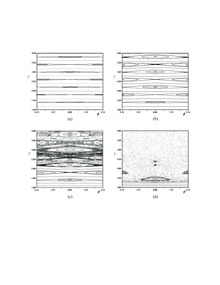
Since the system is of two degrees of freedom, we can study its evolution by using the Poincaré sections $P_{S}=\{(\phi,\gamma),q=0,H=1/2\}$ choosing specific sets of the parameters $a,I,\nu$ and $\theta$. In the numerical calculations, which will follow, we set $I=1$. For the unperturbed system ($a=0$) the sections show invariant curves $\gamma=$const. For $a\neq 0$ some typical examples are shown in Fig.1.

For small values of $a$ (Fig.1a), the invariant curves are perturbed slightly and only close to the most significant resonances their deformation becomes noticeable. Increasing further the perturbation parameter $a$, the width of the resonances increases and homoclinic chaos becomes more obvious close to the hyperbolic fixed points (Fig.1b). The existence of invariant curves, which confine the resonant regions, guarantees the bounded variation of the particle’s energy ($\Delta\gamma=O(\sqrt{a}))$ for the chaotic trajectories.

When the amplitude $a$ exceeds a critical value $a_{c}$, overlapping of resonances takes place and large chaotic regions are generated (Fig.1c) (see also Chirikov (1979)). Particles with initial energy $\gamma$ greater than a critical value $\gamma_{c}$ may follow a chaotic orbit which diffuse to regions of higher energy, and this will lead them to very high energies in short time scales. For relatively large values of $\alpha_{c}<<\alpha<1$, the islands of regular motion, which survive from the resonance overlapping, are gradually destroyed and chaos extends down to relatively low energy particles (Fig.1d). The chaotic part of the phase space will be called “the chaotic sea”.

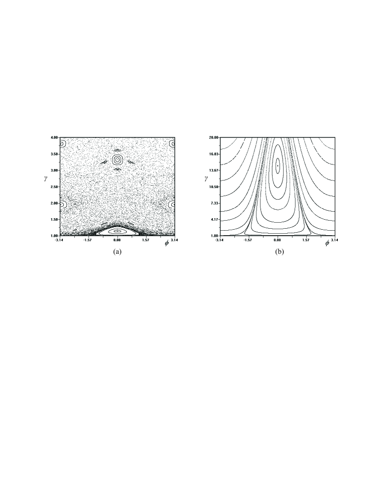
The dynamics, presented by the Poincare sections in Fig.1, is typical for the majority of parameter values. Generally, the critical values $a_{c}$ and $\gamma_{c}$ determine the conditions for possible chaotic diffusion. The dynamics of the charged particles shows some exceptional characteristics when the frequency of the GW is comparable to the Larmor frequency of the unperturbed motion, particularly when $1\leq\nu<3$. For such parameter values, stochastic behavior will appear when $\gamma=1$ and for sufficiently large perturbation values large chaotic regions are generated and diffusion, even for particles with very low initial energies, will be possible. An example is shown in Fig.2a.

The evolution of the particles changes character when the direction of propagation of the GW is almost parallel to $\vec{B}$. In this case, chaos disappears, and the particles undergo large energy oscillations. As it is shown in Fig. 2b, a particle, starting even from rest ($\gamma\approx 1$), will be driven regularly to high energies ($\gamma>20$) and returns back to its initial energy in an almost periodic way. In a realistic, non infinite system, several particles may escape from the interaction with the GW before returning back to low energies. At $\theta=0$ the system is integrable and the energy of the particles shows regular slow oscillations with an amplitude proportional to $a$.

3 Chaotic diffusion and particle acceleration

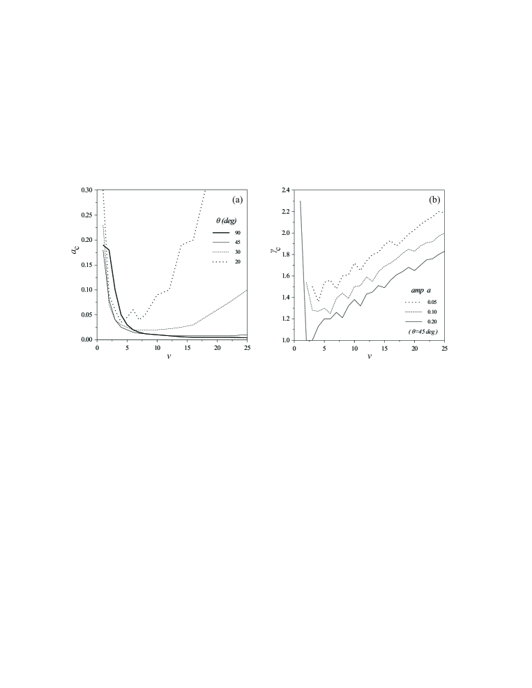
In the previous section, we showed that chaotic diffusion is possible for $a\geq a_{c}$ and for the particles with $\gamma\geq\gamma_{c}$. Such conditions are necessary but not sufficient for acceleration, since islands of regular motion may be present inside the wide chaotic region (see for example Fig. 2). We estimate approximately the critical value $a_{c}$ by studying a large number of Poincaré sections for different values of $\theta$ (Fig.3a). We observe that for small values of $\nu$ resonance overlap is obtained for relatively large amplitudes of the GW. For higher frequency, $\nu>5,$ and $\theta>45$ the overlapping of resonances takes place even for relatively small values of $\alpha$. The critical value $\gamma_{c}$ along the frequency axis $\nu$ is presented for $\theta=45^{o}$ and for $a=0.05,0.1,0.2$ in Fig.3b. For large values of $\nu$, and when the critical value $a_{c}$ is relatively small ($\sim 0.005$), the critical particle energy $\gamma_{c}$ is large and increases linearly with $\nu$. Namely, for large $\nu$, chaotic diffusion takes place only for high energy particles. On the other hand, for $\nu\approx 2$, resonance overlapping takes place for large perturbations but the wide chaotic sea formed extends down to the thermal velocity.

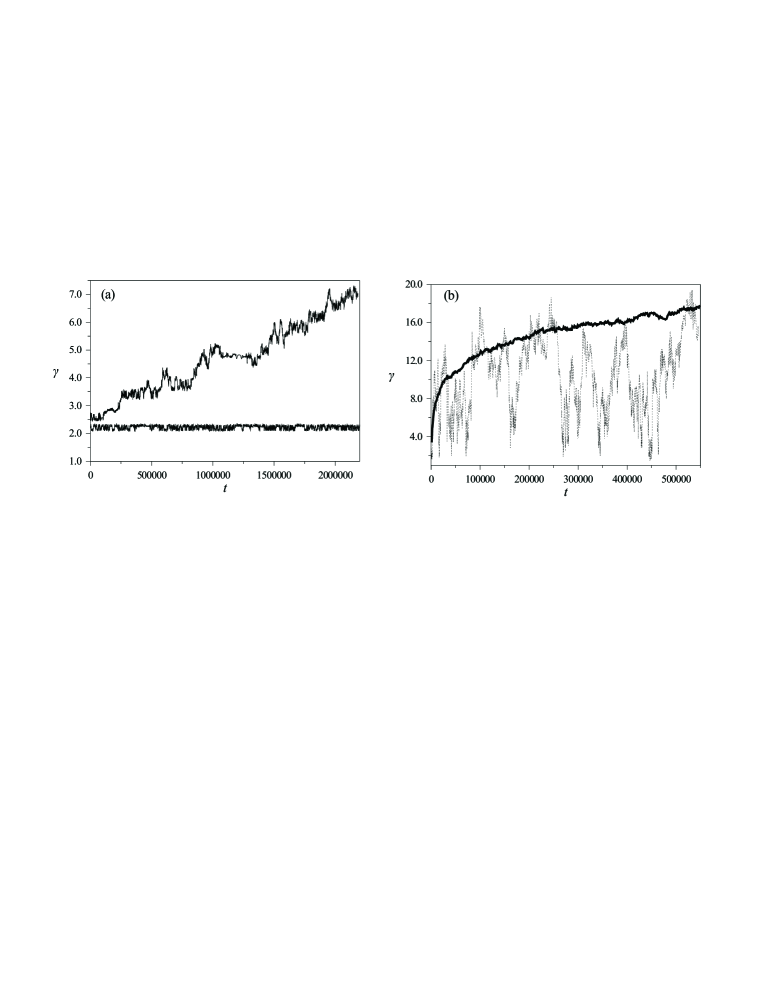
In Fig. 4a the evolution of $\gamma$ along a temporarily trapped chaotic orbit ($\gamma<\gamma_{c}$) and an orbit which undergoes fast diffusion is shown, using $a=0.02$. In Fig. 4b we plot the orbit of a particle which on the average is not gaining energy and the average rate of energy gain of 200 particles. The diffusion rate of the particles in the energy space is initially fast but for time $t>5000$ it starts to slow down. The time $t$ is normalized with the gyro period $2\pi/\Omega$

3.1 GW interacting with an ensemble of electrons

We study next the evolution of an energy distribution $N(\gamma,t=0)$ of electrons interacting with the GW.

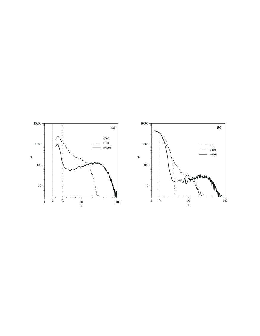
In Fig. 5a we follow the evolution of $3\times 10^{4}$ particles forming initially a cold energy distribution $N(\gamma,t=0)\sim\delta(\gamma-3),$ where $\delta$ is the Dirac delta function i.e. all particles have the same initial energy $\gamma=3.$ A large spread in their energy is achieved in short time scales, and for $t=1000$, a non-thermal tail extending up to $\gamma=100$ is formed.

We repeat the same analysis, assuming that the initial distribution is the tail ($v>V_{the}$, where $V_{the}$ is the ambient thermal velocity) of a Maxwellian distribution (Fig.5b). The distribution of the high energy particle form a long non-thermal tail analogously to the results reported in Fig.(5a).

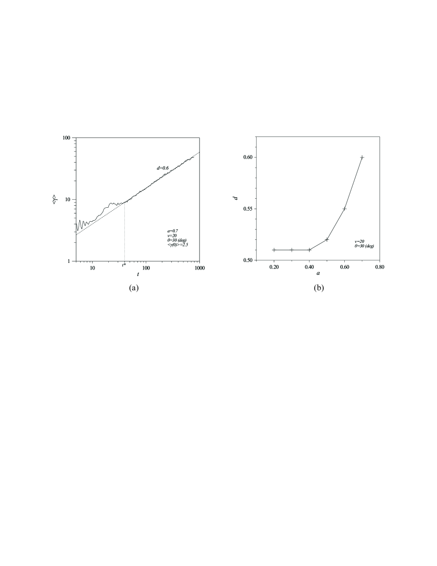
The mean energy diffusion as a function of time is plotted in Fig. 6a for a particular set of parameters, and it has the general form

$$<\gamma>\sim t^{d}.$$ (16)

From a large number of calculations, we find that the energy spread in time follow a normal diffusion ($d=0.5$) in energy space but as $\alpha$ increases (see Fig. 6b), the interaction becomes super-diffusive $(d\geq 0.5)$ in energy space. This allows electrons to spread fast in energy space and explains the efficient coupling between the GW and the plasma.

4 A model for bursty acceleration

Our main findings so far are:

1. The GW can accelerate electrons from the tail of the ambient velocity distribution ($v_{0}(t=0)>V_{the}$) to very high energies ($\gamma>10-100$) for typical values of $0.005<\alpha<0.5$ and $5\leq\omega/\Omega\leq 20.$ Assuming that the the frequency of the GW is around 10KHz, and $\Omega\sim\omega/3$ the magnetic fields strength should be around $\sim 10^{-4}$ Gauss.

2. The acceleration time depends in general on $\alpha$ but is relatively short $t_{acc}\sim 100\Omega^{-1}\sim msecs$. During that time the GW will travel a distance $\ell_{acc}\sim ct_{acc}\sim 10^{8}$ cm.

3. The mean energy diffusion of the electrons interacting with the GW follows the simple scaling $<\gamma>\sim t^{d}.$

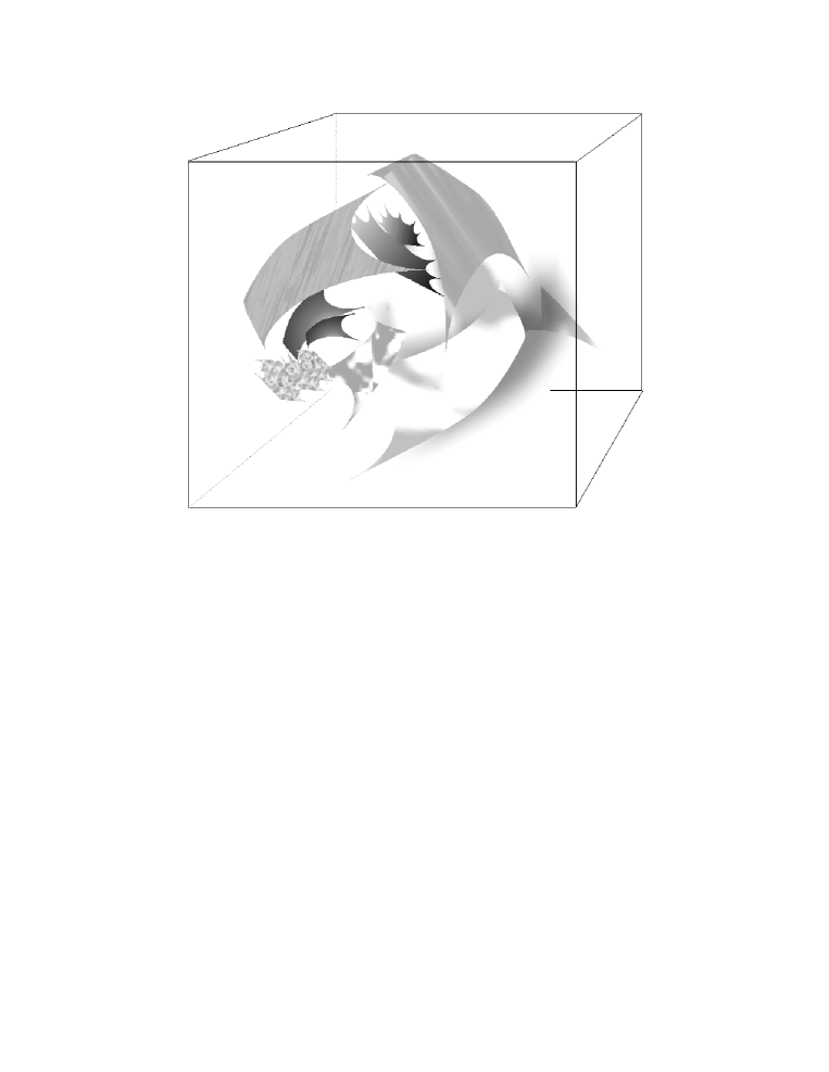
We propose a new mechanism for efficient particle acceleration around strong and impulsive sources of GW using the estimates presented above for the strong interaction of GW with electrons. We assume that in the atmosphere of the central engine a turbulent magnetic field will be formed. Inside this complex magnetic topology, a distribution of 3-D magnetic neutral sheets (magnetic null surfaces) with characteristic length $\ell$ will be developed (see Fig. (7) and the relevant studies for the solar atmosphere (Bulanov and Sakai, 1997; Albright, 1999; Longcop and Klapper, 2002; Longcop et al, 2003)). These 3-D surfaces naturally appear and disappear inside driven MHD turbulent plasmas and are randomly distributed inside the atmosphere of the central engine. It is well known that the neutral sheets will act as localized dissipation regions and will accelerate particles (Nodes et al., 2003). The turbulent atmosphere of the central engine will sporadically emit weak X-ray and possibly $\gamma$-ray bursts for relatively long times before the collapse of the massive magnetized star to form a black hole or the merging of neutron star binaries. We suggest that numerous weak bursts are present and remain unobserved.

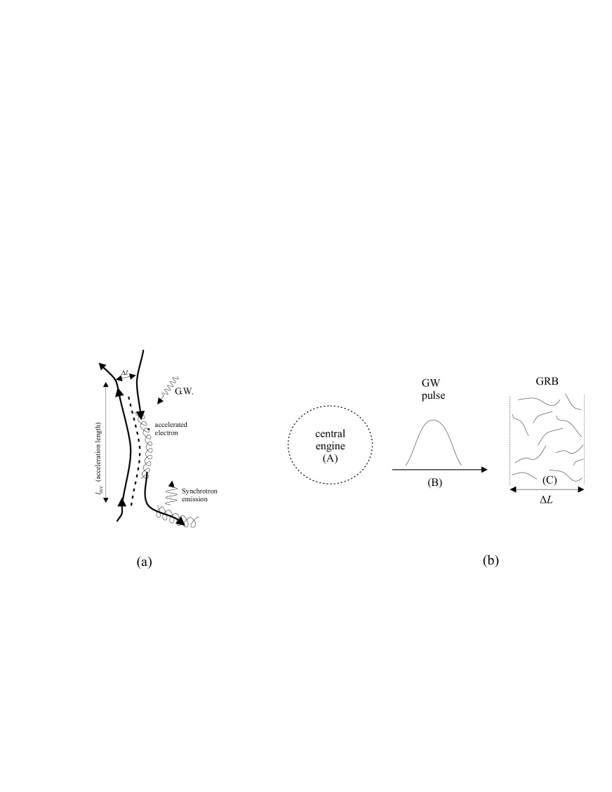
In this article, we emphasize the role of the GW passing through magnetic neutral sheets and claim that the GW will enhance dramatically the acceleration process inside the neutral sheet, causing very intense bursts. According to the arguments presented in sections 2 and 3, the GW can resonate with the electrons only when the magnetic field is weak (in the vicinity of the magnetic null surface). Inside the neutral sheet the synchrotron emission losses are negligible so the acceleration is very efficient. Electrons escaping from the neutral sheet to the super strong magnetic field, expected in the atmosphere of the central engine, transfer very efficiently their perpendicular to the magnetic field energy to synchrotron radiation creating spiky localized bursts. The relativistic electrons retain the parallel to the magnetic field energy and travel along the field lines till they reach the dense ambient plasma and deposit their energy via collisions, causing other types of longer lived bursts (e.g. X-ray and optical flashes)(see Fig. (8a)).

We suggest thus that the creation of a network of localized accelerators with characteristic length $\ell_{acc}$, which are spread in relatively large volumes inside the turbulent atmosphere of the central engine, will be responsible for the busty emission. The amplitude of the GW decays as it propagates away from the central engine as $\alpha\sim 1/r.$ When $\alpha<<a_{c}$ and/or the magnetic topology does not allow formation of magnetic neutral sheets the GW stops to interact with electrons and this indicates the end of the burst. So the overall duration of the burst is approximately $\Delta T\sim\Delta L/c$, where $\Delta L$ is the length of the characteristic layer where the interaction of the GW with the particles is efficient. (see Fig. 8b).

4.1 Energy spectrum

Let us now discuss another very important observational fact. It is well documented that the observed spectrum of the synchrotron radiation has a power law shape. This implies that the energy distribution causing the synchrotron radiation has also a power law dependence in energy

$$N(\gamma)\sim\gamma^{-\varepsilon}$$

were $\varepsilon\simeq 1.8-2.0$ (e.g. see Schaefer et al. (1992) for GRB). These types of energy distribution are usually attributed to a shock wave (or a series of shock waves). The formation of a series of localized shock waves along the streaming plasma injected from the central engine is considered the “standard” model for GRB (Piran, 2003; Mészaros, 2002) and may be of interest in many other astrophysical sources.

The spontaneous formation of magnetic neutral sheets in the 3-D turbulent atmosphere of the central engine is not easy to describe. A number of studies on the statistical properties of the magnetic neutral sheets have appeared for the active region of the Sun (Georgoulis et al., 1998; Longcop and Noonan, 2000; Isliker et al., 2000, 2001; Weatland, 2002; Craig and Wheatland, 2003). All these studies are based on the observational fact that flares follow a specific distribution in energy (Crosby et al., 1993).

An important concept from the study of 3-D MHD turbulence is that a hierarchy of magnetic neutral sheets formed, with a distribution of characteristic lengths given by the function

$$N(\ell)\sim\ell^{-b}.$$ (17)

This scaling follows the energy distribution of flares and the most probable value for $b$ is $3/2$. In other words, inside a turbulent magnetized plasma, a large number of magnetic neutral surfaces with small characteristic lengths, and very few large scale magnetic neutral sheets will be present. The exponent, according to the studies reported earlier, for the solar atmosphere is roughly equal to $b\sim 1-2$ and is related to the statistics of X-ray bursts (Crosby et al., 1993). The GW will accelerate electrons only in the brief period it passes through the magnetic neutral sheet, so the acceleration time will also follow a similar scaling law since

$$t_{acc}\sim\ell_{acc}/c.$$ (18)

We have shown in Fig. 6 that the the mean energy of the accelerated particles increases with time according to a simple power law as well. Combining the Eq. (17)-(18) we derive first the distribution of $t$ which is a function of $\ell$. We have $N(t)\,dt=N(l)\,dl$, or $N(t)=N(l)\frac{d\ell}{dt}$, which yields, when neglecting the constants,

$$N(t)\sim t^{-b}.$$ (19)

We determine next the distribution of $\gamma$ (or, more precisely, of $<\gamma>$), which is a function of $t$. We start again from the relation $N(\gamma)\,d\gamma=N(t)\,dt$, or $N(\gamma)=N(t)\frac{dt}{d\gamma}.$ We insert Eq. (19), $N(\gamma)=t^{-b}\frac{dt}{d\gamma},$ and we replace $t$ on the right hand side using Eq. (16),

$$N(\gamma)=(\gamma^{1/d})^{-b}\frac{d(\gamma^{1/d})}{d\gamma}$$

or, on doing the derivative and rearranging,

$$N(\gamma)=\gamma^{(-b+1-d)/d}.$$ (20)

Using a typical values for $d\sim 0.5$ (see Fig. 6) and $b\sim 3/2,$ we estimate the exponent of the energy distribution to be around 2.

4.2 Energetics

The energy transferred from the GW to the high energy particles by passing through one neutral sheet is

$$\mathbb{E}_{ns}\sim\left(\frac{n_{t}}{n_{0}}\right)n_{0}(\ell_{acc}^{2}\times\Delta\ell)\times\gamma mc^{2}$$ (21)

where $n_{0}$ is the electrons density, $n_{t}$ are the electron at the tail of the local Maxwellian, $\Delta\ell$ is the thickness of the magnetic neutral sheet. The filling factor of neutral sheets inside the atmosphere of the central engine is assumed to be $f.$ So the total number of magnetic neutral sheets expected to interact with the GW is $\frac{(\Delta L)^{3}f}{\ell^{2}\times\Delta\ell}$ and the total energy transferred to the plasma

$$W_{tot}\sim\left[f\times\frac{(\Delta L)^{3}}{\ell^{2}\times\Delta\ell}\right]\times\left(\frac{n_{t}}{n_{0}}n_{0}(\ell_{acc}^{2}\times\Delta\ell)\times\gamma mc^{2}\right).$$ (22)

Using typical numbers $n_{0}=10^{12}\;\textrm{cm}^{-3},n_{t}/n_{0}\sim 10^{-1},\gamma=100,\ell_{acc}\sim 10^{8}\;\textrm{cm},\Delta\ell\sim 10^{7}\;\textrm{cm}\;\;f\sim 10^{-1}$ and assuming that the burst duration is 1s which implies that $\Delta L\sim 3\times 10^{12}\;\textrm{cm},$ the total energy estimated is approximately $10^{47}-10^{48}$ ergs. The total burst duration is around 100s but the burst is composed with many short bursts lasting less than a second ($\ell/c$).

We can now list several characteristics of the bursty emission driven by the model proposed above:

• A fraction of the energy carried by the orbital energy of the neutron stars at merger will go to the the GW and a portion of this energy will be transferred to the high energy electrons.

• The topology of the magnetic field varies from event to event, so every burst has its own characteristics.

• The superposition of many small scale localized sources produces a fine time structure on the burst.

• The superposition of null surfaces with a power law distribution of the acceleration lengths will result in a power law energy distribution for the accelerated electrons and an associated synchrotron radiation emitted by the relativistic electrons.

• The decay of the amplitude of the GW and/or the lack of magnetic neutral sheets away from the central engine will mark the end of the burst, but not necessarily the end of other types of bursts since the cooling of the ambient turbulent plasma has a much longer time scale.

It is worth drawing the analogy between the elements used to build our model for this busrty emission and two significant developments in solar flares and the Earths magnetic tail. (1) Galsgaard and Nordlund, (1997) studied the dynamic formation of current sheets (current sheets are not always associated with neutral sheets) in the solar atmosphere. They found that the irregular motion of the magnetic foot-points, caused by the turbulent convection zone, forces the magnetic topologies to form a hierarchy of 3-D current sheets inside the complex magnetic topologies above active regions. (2) Ambrosiano et al. (1988) studied the passage of low frequency waves (Alfvén waves) through a 2-D neutral sheet. They discovered that the acceleration of charged particles is greatly enhanced from the presence of the Alfvén waves.

We believe that solar flares, the earths magnetotail, and the GW driven bursts share two important characteristics, namely the formation of 3-D magnetic null surfaces coupled with the passage of waves through these surfaces (Alfvén waves for the sun and the earths magnetotail and GW for the bursts analyzed in this article). Although the external drivers and the energetics of the bursts produced are clearly very different.

5 Summary

In this article we have study an efficient mechanism to transfer the energy released from a central engine to the turbulent plasma in its atmosphere. We have analyzed the non-linear interaction of GW with electrons. We showed that electrons in the tail of the ambient plasma are accelerated efficiently, reaching energies up to hundreds of MeV in less than a second, when (1) the amplitude of the GW is above a typical value $0.005-0.5$ and (2) the magnetic field is relatively weak $B_{0}\sim 10^{-4}$ Gauss, for a GW with typical frequency 1-10KHz.

On the basis of these findings, we propose that pulsed GW emitted from the central engine will interact with the ambient plasma in the vicinity of the magnetic neutral sheets formed naturally inside externally driven turbulent MHD plasmas. Magnetic neutral sheets have characteristic lengths $\ell\sim 10^{7}-10^{8}$ cm and are short lived 3-D surfaces. Although these structures are efficient accelerators, we are emphasizing in this article only the role of the GW passing through these surfaces since we focus our attention on the very strong and bursty sources. The GW passing through the neutral sheets will accelerate electrons to very high energies. Relativistic electrons escape from the magnetic neutral sheets radiating synchrotron emission as soon as they reach the very strong magnetic fields.

The collective emission of thousands of short lived (less than a second) synchrotron pulses, created during the passage of the GW through a relatively large volume. The relativistic electrons loosing most of their perpendicular to the magnetic field energy to synchrotron radiation retain the parallel energy and heat the ambient plasma emitting other types of longer lived bursts, e.g. X-rays and optical flushes.

We have also shown that if the acceleration length follows a simple scaling law ($N(\ell_{acc})\sim\ell_{acc}^{-b}$) and since, as shown, $<\gamma>\sim t_{acc}^{d},$ the energy distribution also follows a power law scaling ($N(<\gamma>)\sim<\gamma>^{(-b+1-d)/d}$), which for reasonable values of $b\sim 3/2$ and $d\sim 1/2$ agrees remarkably well with the energy distributions inferred from the observations.

We are suggesting that numerous burst are still present before and after the passage of the GW since the magnetic neutral sheet act as efficient particle accelerators. The GW passage simply enhances the acceleration process and makes many short lived spikes to become visible. We propose that a more thorough analysis of the statistical properties of the bursty emission, with main emphasis on the low energy part of the frequency distribution, will give important insight on the processes mentioned here.

A detailed model for the interaction of GW with turbulent MHD plasma is currently under study, and we hope to develop an even more efficient energy transfer from the GW to the plasma e.g by triggering the interaction (percolation) of many null sheets during the passage of the GW. We hope that this may lead us to an alternative scenario for the still unresolved questions related with the acceleration mechanism in the atmosphere of the central engines and the physical processes behind the X-ray and GRB.

Figure 1: Typical Poincaré sections on the plane ($\phi,\gamma$) of the perturbed system for $\nu=5,\theta=45^{o}$ and a) $a=0.001$ b) $a=0.01$ c) $a=0.02$ and d) $a=0.1$.

Figure 2: Poincaré sections on the plane ($\phi,\gamma$) a) $a=0.2,\nu=2,\theta=45^{o}$ b)$a=0.2,\nu=1,\theta=5^{o}$.

Figure 3: a) The variation of critical value $a_{c}$ with the angular frequency $\nu$ of the GW.   b) The same for the critical value $\gamma_{c}$ and $\theta=45,$ using typical values for the amplitude $a$.

Figure 4: a) The evolution of $\gamma$ along a trapped in a magnetic island chaotic orbit for $\gamma(0)=2.2$,$\phi(0)=\pi$ and along a diffusive one for $\gamma(0)=2.6$, $\phi(0)=0$ ($a=0.02,\theta=45^{o},\nu=5$) b) The evolution of $\gamma$ along a strongly chaotic orbit (dotted line) and its average value (solid line) along 200 trajectories starting with $\gamma(0)=2.0$ and a randomly selected $\phi(0)$ ($a=0.1,\theta=45^{o},\nu=5$). The time is normalized with the gyro-period $(2\pi/\Omega)$.

Figure 5: The evolution of an energy distribution. a) The initial distribution (dotted line) consists of $3\times 10^{4}$ particles having $\gamma(t=0)=3.$ b) The initial distributions is Maxwellian, as it is shown by the dotted curve. Only particles in the tail of the Maxwellian with $\gamma>\gamma_{c}$ will be accelerated. The parameters used in both studies are $a=0.5$, $\nu=20$ and $\theta=30^{o}$.

Figure 6: (a) We plot the mean energy diffusion in time. We observe that $\log(<\gamma>)$ is linearly related to $\log(t)$ for $t>t^{*}$. The slope $d$ for $\alpha=0.7$ is $d\sim 0.6.$ (b) The slope $d$ is plotted as a function of the GW amplitude.

Figure 7: A schematic representation of the thin three dimensional magnetic null sheets appearing spontaneously and fill densely a driven turbulent magnetized plasma

Figure 8: (a) The propagation of a GW through a magnetic neutral sheet accelerates electrons very efficiently. Relativistic electrons stream away from the accelerator and emit a pulse of synchrotron radiation when they reach the super strong magnetic fields. The dashed line represents the magnetic field null surface and $\ell_{acc}$ is the acceleration length. (b) A collection of magnetic neutral sheets is formed inside the turbulent atmosphere (region C) of the central engine (region A). A GW pulse propagating away from the central engine and passing through the region C will form numerous $\gamma$-ray spikes by accelerating particles near the magnetic null surfaces. The superposition of these spikes form a short lived burst. The total burst duration is approximately 100s ($\Delta T\sim\Delta L/c$) but it is composed by many short spikes lasting less than a second ($\ell/c$). The GW pulse will become very weak and the density of the magnetic null surfaces will drop dramatically in the region D, and this will mark the end of the burst.

References

- Albright (1999) Albright, B.J., 1999, Phys. Plasmas, 6, 4222
- Ambrosiano et al. (1988) Ambrosiano, J., Matthaeus, W., Goldstein, M.L., Plante, D., 1988, J. Geoph. Res., 93, 14383.
- Arnol’d, et al. (1987) Arnol’d, V.I, . Kozlov, V.V., Neishtadt,A.I, 1987, Mathematical aspects of classical and celestial Mechanics, in Dynamical Systems III, ed. V.I. Arnol’d, Springer-Verlag: Berlin.
- Baumgarte and Shapiro (2003) Baumgarte, T.W., Shapiro, S.L., 2003, ApJ, 585, 930.
- Brodin and Marklund (1999) Brodin, G., Marklund, M., 1999, Phys. Rev. Let. 82, 3012
- Brodin et al. (2000) Brodin, G., Marklund, M., Dunsby, P.K., M. 2000, Phys. Rev. D 62, 104008
- Brodin et al. (2001) Brodin, G., Marklund, M., Servin, M. 2001, Phys. Rev. D 63, 124003
- Bulanov and Sakai (1997) Bulanov, S.V., Sakai, J-I., 1997, J. Phys. Soc. Japan, 66, 3477.
- Chirikov (1979) Chirikov B.V., 1979, Phys. Rep., 52, p.264.
- Cooperstock (1968) Cooperstock, F.I. 1968, Ann. Phys. 47, 173
- Craig and Wheatland (2003) Craig, I.J.D., Wheatland, M., 2003, Sol. Phys., 211, 275
- Crosby et al. (1993) Crosby,N.B., Aschwanden, N.J., Dennis, B.R., 1993, Sol. Phys., 143, 275.
- Daniel and Tajima (1997) Daniel, J., Tajima, T., 1997, Phys. Rev., D. 55, 5193.
- Demianski (1985) Demianski, M. 1985, Relativistic Astrophysics, Pergamon Press, Oxford, UK
- Denisov (1978) Denisov, V.I. 1978, Sov. Phys. JETP 42, 209
- DeWitt and Breheme (1960) DeWitt, B.S., Breheme, R. W. 1960, Ann. Phys. 9, 220
- Dimmelmeir et al. (2002) Dimmelmeier, H., Font, A.J., Muller, E., 2002, A$A, 393, 523.
- Fryer et al. (2002) Fryer, C.L., Holz, D.E., Hughes, S.T., 2002, ApJ, 565, 430
- Galsgaard and Nordlund, (1997) Galsgaard, K. & Nordlund, A., 1997, J. Geophys. Res., 102, 231.
- Georgoulis et al. (1998) Georgoulis, M. K., Velli, M., Einaudi, G., 1998, ApJ, 497, 957
- Gerlach (1974) Gerlach, U. H. 1974, Phys. Rev. Lett. 32, 1023
- Gertsenshtein (1962) Gertsenshtein, M.E. 1962, Sov. Phys. JETP 14, 84
- Grishchuk and Polnarev (1976) Grishchuk, L.P., Polnarev, A.G. 1976, in General Relativity and Gravitation, Vol. 2, ed. A.Held, Plenum Press.
- Isliker et al. (2000) Isliker, H., Anastasiadis, A., Vlahos, L., 2000, A&A, 363, 1134
- Isliker et al. (2001) Isliker, H., Anastasiadis, A., Vlahos, L., 2001, A&A, 377, 1068.
- Kleidis et al. (1993) Kleidis, K., Varvoglis, H., Papadopoulos, D., 1993, A&A, 275, 309.
- Kleidis et al. (1995) Kleidis, K., Varvoglis, H., Papadopoulos, D., Esposito, F.P., 1995, A& A, 294, 313.
- Shibata and Uryu (2002) Shibata, M., Uryu, K., 2002, Prog. Theor. Phys., 107, 265.
- Longcop and Noonan (2000) Longcop, D.W., Noonan, E.J., 2000, ApJ, 542, 10088
- Longcop and Klapper (2002) Longcop, D.W., Klapper, I., 2002, ApJ, 579,468
- Longcop et al (2003) Longcope, D.W., Brown, D.S. & Priest, E.R., 2003, Phys. Plasmas, 10, 3321
- Macdonald and Thorne (1982) Macdonald, D., Thorne, K.S. 1982, MNRAS 198,345
- Macedo and Nelson (1982) Macedo, P.G., Nelson, A. G. 1982, Phys. Rev. D. 28, 2382
- Marklund et al. (2000) Marklund, M., Brodin, G., Dunsby, P.K.S. 2000, ApJ 236, 875
- Mészaros (2002) Mészaros, P., 2002, Annual Rev. Astr. & Ap.,
- Misner et al. (1973) Misner C.W., Thorne K.S. & Wheeler J.A., 1973, Gravitation, Freeman, San Francisco.
- Moortgat and Kuijpers (2003) Moortgat, J., Kuijpers, J., (2003), A&A, 402, 905
- Nodes et al. (2003) Nodes, C., Birk, G.T., Lesch, H., Schopper, R., 2003, Plasma Phys., 10, 835.
- Ohanian (1976) Ohanian H.C., 1976, Gravitation and Spacetime, Norton & Company, New York.
- Papadopoulos and Esposito (1981) Papadopoulos D., Esposito F., 1981, ApJ 248, p.783.
- Papadopoulos et al. (2001) Papadopoulos, D., Stergioulas, N., Vlahos, L., Kuijpers, J., A&A, 2001, 377, 701.
- Polanrev (1972) Polnarev, A.G. 1972, Sov. Phys. JEPT 35, 834
- Piran (2003) Piran, T., 2003, astro-ph/9810256
- Ruffert and Janka (1998) Ruffert, M., Janka, H.T., 1998, A&A, 338, 53.
- Sagdeev, et al. (1988) Sagdeev,R.Z., Usikov,D.A., Zaslavsky, G.M.: Nonlinear Physics (Harwood Academic 1988)
- Schaefer et al. (1992) Schaefer et al., 1992, in Fishman, G.J., Brainerd, J.J., Eds., Gamma-Ray Bursts 2nd Hundsvill Symposium, AIP Conf. Proc. 307 (NY).
- Servin et al. (2000) Servin, M., Brodin, G., Bradley, M., Marklund, M., 2000, Phys. Rev., E 62, 8493.
- Servin et al. (2001) Servin, M., Brodin, G., Marklund, M., 2001, Phys. Rev., D 64, 024013.
- Varvoglis and Papadopoulos (1992) Varvoglis, H., Papadopoulos, D., 1992, A&A 261, 664
- Weatland (2002) Weatland, M., 2002, Sol. Phys., 208, 33
- Zaslavsky (2002) Zaslavsky, G.M., Phys. Rep., 2002, 371, 461
- Zeld́ovich (1974) Zel’dovich, Y. B. 1974, Sov. Phys. JETP 38, 652