XMM-Newton observations of 3C 273

Abstract

A series of nine XMM-Newton observations of the radio-loud quasar 3C 273 are presented, concentrating mainly on the soft excess. Although most of the individual observations do not show evidence for iron emission, co-adding them reveals a weak, broad line (EW $\sim$ 56 eV). The soft excess component is found to vary, confirming previous work, and can be well fitted with multiple blackbody components, with temperatures ranging between $\sim$ 40 and $\sim$ 330 eV, together with a power-law. Alternatively, a Comptonisation model also provides a good fit, with a mean electron temperature of $\sim$ 350 eV, although this value is higher when the soft excess is more luminous over the 0.5–10 keV energy band. In the RGS spectrum of 3C 273, a strong detection of the Ovii He$\alpha$ absorption line at zero redshift is made; this may originate in warm gas in the local intergalactic medium, consistent with the findings of both Fang et al. (2003) and Rasmussen et al. (2003).

1 Introduction

3C 273 was the first object positively identified as a quasar, in 1963: the radio source was identified with a magnitude 13, star-like object by Hazard, Mackey & Shimmins (1963) and the redshift measured by Schmidt (1963) to be z = 0.158. 3C 273 was later found to be a X-ray source, by Bowyer et al. (1970) and Kellogg et al. (1971), and has been observed with X-ray instruments ever since. It is a radio-loud quasar, with a jet showing superluminal motion. Although many more quasars have been discovered since the 1960s, 3C 273 remains one of our nearest neighbours; this, therefore, makes it a prime object to study, over the entire range of the electromagnetic spectrum; see Courvoisier (1998) and references therein. Previous X-ray observations found the high-energy continuum could be fitted by a hard power-law, with a variable photon index, $\Gamma$ $\sim$ 1.3–1.6 (Turner et al. 1990; Turner et al. 1991; Williams et al. 1992). Observations by EXOSAT (Turner et al. 1985) first indicated the existence of a soft excess, at energies $\mathrel{\raise 1.29167pt\hbox{$<$}\mkern-14.0mu\lower 2.58334pt\hbox{$\sim$}}$ 1 keV; this was subsequently confirmed by further EXOSAT observations (Courvoisier et al. 1987; Turner et al. 1990), together with data from Einstein (Wilkes & Elvis 1987; Turner et al. 1991), Ginga (Turner et al. 1990) and ROSAT (Staubert 1992). Beppo-SAX (Orr et al. 1998) and ASCA (Yaqoob et al. 1994; Cappi et al. 1998) have also observed 3C 273, along with EUVE, which allowed the soft excess to be detected down to $\sim$ 0.1 keV (Marshall et al. 1995). The actual form of the soft excess could not previously be determined, due to lack of precision in the low-energy instruments: power-law, blackbody and thermal Bremsstrahlung models produced equally acceptable fits. The EPIC (European Photon Imaging Camera) instruments (Strüder et al. 2001; Turner et al. 2001) on board XMM-Newton are improving the situation, however, helping to distinguish between different models much more readily.

The soft excess of 3C 273 has been previously found to vary (Turner et al. 1985; Courvoisier et al. 1987; Turner et al. 1990; Grandi et al. 1992; Leach, McHardy & Papadakis 1995); Ginga observations (Saxton et al. 1993) found that its fractional variability was larger than that in the corresponding power-law component.

In this paper, nine XMM observations of 3C 273 are presented. In Section 2 the XMM datasets are given and the problem of pile-up discussed. Section 3 covers the spectral analysis, concentrating in particular on the soft excess emission. Sections 4 and 5 cover the RGS (Reflection Grating Spectrometer) and optical data respectively, while Section 6 discusses what can be determined from the spectral fits, with the final conclusions given in Section 7. Throughout the paper, H₀ is taken to be 50 km s^-1 Mpc^-1 and q₀ = 0.

2 XMM-Newton Observations

3C 273 is one of the XMM-Newton calibration targets, so is frequently observed by the instruments. At the time of writing, the quasar has been observed in revolutions 94, 95, 96, 277, 370, 373, 382, 472, 554 and 563, spanning a time period of two and half years, from 2000-06-13 to 2003-01-05. These data are a combination of public and proprietary calibration observations. Since the PN was in Timing mode during revolution 382, this observation was excluded from the analysis; MOS 1 was in Timing mode for four of the nine observatiosn, so only MOS 2 data were used. The observation during revolution 472 is considerably shorter than the others; this, combined with the low luminosity of 3C 273 at this time, leads to larger error bars than measured during the other revolutions. Table 1 lists the dates of the observations, together with the exposure times and instrumental set-up. The ODFs (Observation Data Files) were obtained from the online Science Archive; the data were then processed and the event-lists filtered using xmmselect within the sas (Science Analysis Software) v5.4.1.

Table 1: The details of the XMM observations of 3C 273 analysed in this sample. For revolution 563, the two MOS 2 observations were summed. The ‘clean’ exposure times are given, i.e. those after the periods of high background have been removed. Revolution 472 has about half the exposure of the next shortest observation.

Rev.	Obs. ID	start date	exposure time (ks)		filter
			MOS 2	PN	MOS 2	PN
94	0126700301	2000-06-13	53.4	39.7	medium	medium
95	0126700701	2000-06-15	27.7	19.6	medium	medium
96	0126700801	2000-06-17	42.6	31.8	medium	medium
277	0136550101	2001-06-13	41.7/36.6	30.1	medium/thin	medium
370	0112770101	2001-12-16	4.3	3.1	medium	thin
373	0112770201	2001-12-22	4.1	3.0	medium	thin
472	0112770601	2002-07-07	2.3	1.7	medium	thin
554	0112770801	2002-12-17	4.5	3.3	medium	thin
563 (i)	0136550501	2003-01-05	7.9	5.7	medium	medium
563 (ii)	0112770701	2003-01-05	4.6	3.3	medium	thin

Only Small Window Mode observations were used, to minimise the pile-up problems. Upon investigation, it was found that the MOS spectra were slightly piled-up, even with the quicker read-out time from the Small Window. Figure 1 shows the output from the sas task epatplot; the panel compares the expected fractions of single-, double-, triple- and quadruple-pixel events (solid line) with those actually measured in the spectrum (histogram). It can be seen that a smaller than expected fraction of single events is measured above $\sim$ 1 keV, while the reverse is true for doubles; this is the main signature of pile-up.

Pulse pile-up in CCD cameras occurs when there is a significant probability that two or more photons registering within a given CCD frame will have overlapping charge distributions. This can lead to a spectral distortion if the resulting charge distribution is recognised as a single event whose energy is the sum of the overlapping events, or a flux loss if the charge distribution has a pattern which is not within the detector’s pattern library. The dominant effect of moderate pile-up in the MOS cameras is a loss of flux, with little, or no, spectral distortion, especially if single-pixel events only are analysed. The degree of pile-up for a given point source depends on the source strength and also the point-spread function, throughput, pixel size and frame accumulation time of the given X-ray detector system. Approximate limiting count rates are quoted in the XMM User Handbook for the MOS and PN small window modes of 5 and 130 counts s^-1, respectively.

3C 273 has a typical 0.1-10 keV count rate of between 10/35 and 20/65 counts s^-1 for MOS/PN respectively, and is therefore moderately piled-up in the MOS but only very weakly piled-up (if at all) in the PN. Spectral distortion due to pile-up can be reduced by only analysing single pixel events, although there is a trade-off in sensitivity. The spectral fitting has, therefore, been restricted to single pixel events in both cameras. The MOS single pixel spectra have also been corrected for residual pile-up effects using the method described in Molendi and Sembay (2003). This method uses the fact that the majority of diagonal bi-pixel events within a source box are created by the pile-up of two single pixel events. The observed diagonal bi-pixel events spectrum can then be used to correct the observed single pixel spectrum. Additionally, a development version of the MOS response matrix was used for the observations, which has reduced the systematic errors in the low energy ($<$ 2 keV) band; this is expected to be included in the next sas release.

The MOS 2 and PN data were then fitted simultaneously and the results are presented in the following sections. There are well-known systematic differences between MOS and PN fitted spectral parameters, arising from their imperfect calibration and, at this stage, it is not clear which instrument has the smaller systematic errors. The statistical precision of the 3C 273 observations is such that these systematic errors dominate. The practical solution adopted here is to carry out joint fits to MOS and PN, allowing the normalisation to float in order to take care of the differing degrees of flux-loss due to pile-up in the two instruments. Individual fits to the MOS and PN data give better $\chi^{2}_{\nu}$s, but different parameter values, caused by the calibration uncertainties. For example, over 3–10 keV, there is a slight difference in power-law slopes, with $\Delta\Gamma$ $\leq$ 0.1, but using blackbodies to fit the soft excess led to noticeably different temperatures; e.g., $\sim$ 95 and 240 eV for PN, compared to $\sim$ 130 and 400 eV for MOS. However, the joint fits are acceptable on the basis of $\chi^{2}$ alone.

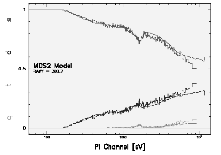
Figure 1: This plot shows the result of running epatplot on the MOS 2 spectrum of 3C 273 in revolution 96. The top curve shows the expected (solid line) and observed (histogram) fractions of single-pixel events, while the corresponding results for the double events are shown just below. The lowest lines correspond to triple and quadruple events. There are fewer single-events, but more doubles, observed than are predicted; this shows the data are piled-up.

3 Spectral Analysis

3.1 Iron lines

The object of this paper is to analyse the soft excess of 3C 273 and to investigate any spectral changes there may be over time. The possible presence of an iron emission line was, however, investigated, by fitting the MOS 2 and PN spectra over the 3–10 keV range with a simple power-law model. On the whole, iron lines, either narrow or broad, were not detected in the individual pointings; the limits on the equivalent widths are given in Table 2. An alternative way to analyse the possible changes in the iron emission is to compare the line fluxes for different observations; this separates any variability due to the continuum from the intrinsic line variabilty. The values are also given in Table 2, where it can be seen that they are consistent with a constant line flux.

The spectra from all nine observations were then co-added, to search for the possible presence of an iron line; this resulted in a spectrum with a total exposure time of almost 193 ks for the MOS and 127 ks for the PN. (Only those observations taken with the medium filter were used.) As Table 3 and Figure 10 show, the 3–10 keV spectral index does not vary greatly between observations ($\Gamma$ lies between 1.64 and 1.78); this is important, since co-adding spectra with different slopes would lead to curvature and, hence, force a broad residual when fitting a simple power-law model.

There is some evidence for a narrow line (E = 6.34 $\pm$ 0.03 keV; EW = 8 $\pm$ 3 eV; $\Delta\chi^{2}$ = 18 for 2 degrees of freedom), but the evidence for a weak broad line was significantly better ($\Delta\chi^{2}$ of 57 for 3 degrees of freedom), giving an equivalent width of 56 $\pm$ 19 eV, for E = 6.37 $\pm$ 0.09 keV and $\sigma$  = 0.60 $\pm$ 0.11 keV. Adding an absorption edge (E = 7.30 $\pm$ 0.07 keV; $\tau$ = 0.04 $\pm$ 0.01) further imrpoves the fit ($\Delta\chi^{2}$ of 15 for 2 degrees of freedom), giving a final reduced $\chi^{2}$ value of 1451/1728. Figure 2 shows this broad line clearly above a simple power-law model, fitted above 3 keV, while Figure 3 plots the confidence contours for the energy of the line. The implies that the line is not strongly ionised.

Iron emission in 3C 273 was first identified by Ginga (Turner et al. 1990), where a line of EW $\sim$ 50 eV was detected, although the width could not be constrained. At the time of the Ginga observation, the 2–10 keV luminosity of the source was measured to be $\sim$ 7 $\times$ 10⁴⁵ erg s^-1, showing 3C 273 to be somewhat fainter than in the present observations (Table 3). Note that the luminosities tabulated here are over the narrower energy band of 3–10 keV. A weak and broad, but ionised, line was reported by Yaqoob & Serlemitsos (2000), who detected such a component in RXTE and ASCA observations of 3C 273. Kataoka et al. (2002) also confirmed the presence of a broad line in earlier RXTE data. In the present data, the line appears to be neutral (Figure 3). The EW of $\sim$ 50 eV found in the present data is consistent with these earlier observations. Superluminal blazars, such as Mrk 421, show no hint of iron lines in their X-ray spectra (e.g., Brinkman et al. 2001); these are sources which are very probably being viewed directly down the radio jet. 3C 273 is oriented such that the radio lobes are visible, although superluminal motion is still observed. The presence of the iron line indicates that a Seyfert-like disc spectrum is being seen in 3C 273.

In a recent paper (Page et al. 2003), the decrease in strength of narrow lines with luminosity (i.e., the X-ray Baldwin effect) was discussed. The fact that, in the coadded data presented here, a broad line is preferable to a narrow component is in agreement with this finding. There is also a Baldwin effect for broad lines such as the one measured here (Nandra et al. 1997), which are thought to be produced through reflection off the inner accretion disc; the low EW found for the weak broad line here supports this result.

Table 2: The limits on the equivalent widths (EW) of neutral (6.4 keV) and ionised (6.7 keV) iron emission in 3C 273. The narrow lines had an intrinsic width of $\sigma$ = 0.01 keV, the broad lines, 0.5 keV. Where the line was less than 99 per cent significant, the 90 per cent upper limit is given. The other error bars are at the 1$\sigma$ level.

^a flux in units of 10^-13 erg cm^-2 s^-1

Rev.	Narrow Line		Broad Line
	(neutral)		(neutral)		(ionised)
	EW (eV)	line fluxa	EW (eV)	line fluxa	EW (eV)	line fluxa
94	$<$9	$<$ 0.77	47 $\pm$ 13	3.98 $\pm$ 1.49	$<$51	$<$4.16
95	$<$10	$<$ 0.84	54 $\pm$ 19	4.39 $\pm$ 1.66	42 $\pm$ 20	3.29 $\pm$ 1.73
96	$<$17	$<$1.42	71 $\pm$ 20	5.84 $\pm$ 1.66	71 $\pm$ 22	5.62 $\pm$ 1.73
277	$<$12	$<$1.20	$<$40	$<$4.15	$<$33	$<$3.32
370	$<$28	$<$3.26	$<$81	$<$9.37	$<$110	$<$12.33
373	$<$41	$<$4.74	$<$136	$<$15.60	$<$121	$<$13.49
472	$<$74	$<$5.83	$<$166	$<$13.00	$<$101	$<$7.80
554	$<$36	$<$3.86	$<$147	$<$15.50	$<$144	$<$14.74
563	$<$21	$<$1.79	$<$72	$<$6.17	$<$69	$<$5.75

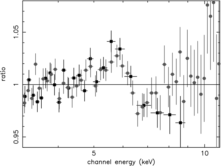
Figure 2: A weak broad line can be seen in the co-added spectrum of all nine observations. The MOS data points are shown as squares, the PN as circles.

Figure 3: A contour plot for the broad line, showing the 68, 90, 95 and 99 per cent (innermost to outermost curves) possibilities for the energy of the line, for two degrees of freedom. The plot shows that the line is not strongly ionized.

3.2 The soft excess

As is conventional, after fitting a power-law with Galactic absorption (N_H = 1.79 $\times$ 10²⁰ cm^-2; obtained from the ftool nh, which derives the value from Dickey & Lockman 1990) to the 3–10 keV energy band (to avoid the broad soft excess), the fit was extrapolated down to 0.5 keV. (The MOS and PN calibration differences increase rapidly below this point, so lower energy data have not been used.) There is an obvious soft excess, of which Figure 4 shows an example.

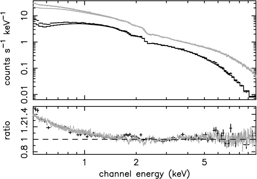
Figure 4: An extrapolation of the power-law fitted over the 3–10 keV band (Table 3) shows the soft excess of 3C 273, during revolution 95. Both MOS 2 (black) and PN (grey) data are shown.

The soft excess of 3C 273, as observed by EPIC, can be well modelled by multiple blackbody (BB) components. Considering the revolution 95 data as an example, fitting the broad-band spectrum with a power-law together with a single BB component gives an unacceptable fit, with $\chi^{2}$/dof = 2782/2279. Adding a second BB gives the best-fit value of 2546/2277; the F-test value for this improvement is 18. When using the F-test, a value of F $>$ 3.0 (for one parameter) corresponds to an improvement of $>$ 90 per cent.

Table 3 gives the 3–10 keV power-law slopes, together with broad-band BB fits; Fig. 5 shows an example of the unfolded BB fit. During revolution 277, observations with both the thin and medium MOS filters were performed, while the same was done for PN during revolution 563; the spectra from the different filters were fitted simultaneously, using the appropriate filter responses, leading to the increased number of degrees of freedom seen in the table. The last column of the table lists the unabsorbed luminosities for the models given. These values show 3C 273 to have been at a typical luminosity during each of the observations, c.f. Courvoisier et al. (1987).

Figure 5: An unfolded plot of the blackbody fit to the revolution 95 data. The spectrum is fitted by a power-law and two blackbody components, with kT $\sim$ 91 and 232 eV (see Table 3).

Table 3: Power-law and blackbody fits to the MOS 2 and PN 3C 273 spectra. The unabsorbed luminosities are also given in the final column, for the corresponding bandpasses.

Range	Model	Rev.	$\Gamma$	kT (keV)	kT (keV)	kT (keV)	$\chi^{2}$/dof	luminosity
(keV)								(1046 erg s-1)
3–10	PL	94	1.679 $\pm$ 0.007				1729/1583	0.79
		95	1.674 $\pm$ 0.008				1581/1543	0.77
		96	1.643 $\pm$ 0.008				1685/1548	0.76
		277	1.643 $\pm$ 0.006				2364/1946	0.95
		370	1.675 $\pm$ 0.021				901/840	1.08
		373	1.696 $\pm$ 0.021				818/839	1.08
		472	1.772 $\pm$ 0.035				464/389	0.74
		554	1.776 $\pm$ 0.022				873/817	1.00
		563	1.771 $\pm$ 0.014				1469/1525	0.81
0.5–10	PL + BBs	94	1.679 $\pm$ 0.005		0.100 $\pm$ 0.003	0.252 $\pm$ 0.011	2802/2331	1.68
		95	1.674 $\pm$ 0.020		0.091 $\pm$ 0.004	0.232 $\pm$ 0.010	2546/2277	1.62
		96	1.643 $\pm$ 0.006		0.094 $\pm$ 0.003	0.234 $\pm$ 0.012	2701/2256	1.60
		277	1.648 $\pm$ 0.006	0.039 $\pm$ 0.002	0.117 $\pm$ 0.004	0.277 $\pm$0.010	3833/2741	2.06
		370	1.700 $\pm$ 0.018		0.100 $\pm$ 0.006	0.279 $\pm$ 0.028	1615/1428	2.38
		373	1.699 $\pm$ 0.017		0.095 $\pm$ 0.007	0.261 $\pm$ 0.027	1621/1426	2.33
		472	1.779 $\pm$ 0.035		0.098 $\pm$ 0.010	0.330 $\pm$ 0.051	1134/928	1.70
		554	1.798 $\pm$ 0.019		0.098 $\pm$ 0.006	0.288 $\pm$ 0.0024	1610/1402	2.33
		563	1.806 $\pm$ 0.012		0.103 $\pm$ 0.005	0.257 $\pm$ 0.016	2587/2562	1.91

Modelling the soft excess spectrum with multiple blackbodies is probabaly not physical, but it does point to the soft excess being broad. The diskbb model in Xspec models the accretion disc as emission from multiple blackbody components, working from the temperature at the inner disc radius (see, e.g., Mitsuda et al. 1984; Makishima et al. 1986). However, this method does not succeed in modelling the entire breadth of the emission seen, and was worse than either multiple BB (F = 77, if BB are substituted; $\Delta\chi^{2}$/dof = 171/2) or the Comptonisation fits (see below). An alternative method involves modelling the soft excess with either a second, or a broken, power law. However, both of these models were found to be significantly worse fits (the F-test gives improvements of 254 and 124 for the multiple blackbodies in comparison to the two power-laws and broken power-law respectively, for revolution 95 data; these correspond to $\Delta\chi^{2}$/dof of 569/2 and 277/2 respectively), implying that the soft excess does, indeed, show curvature, rather than a sharp change in slope.

As mentioned above, although multiple blackbodies parametrize AGN soft excesses very well, the model is not particularly physical. The temperatures for the hotter components are thought to be far higher than can be formed through thermal emission from an accretion disc surrounding a $\sim$ 10${}^{9}{\rm M_{\odot}}$ black hole (see, e.g., Liu et al. 2003). A more realistic model for the emission is likely to be Comptonisation: thermal photons, emitted from the disc, are upscattered by populations of hot electrons. A two-temperature distribution could then lead to the formation of both the apparent ‘power-law’ at higher energies and the soft excess. Low temperature Comptonised spectra are similar in shape to blackbodies, but are broader; thus, an excess which requires two or three different temperature BBs can easily be modelled by a single Comptonisation component.

To investigate the likelihood of the 3C 273 spectra being formed via this method, the thCompfe Comptonisation model (Życki, Done & Smith 1999) was utilised. Blaes et al. (2001) fit an accretion disc model to multi-wavelength 3C 273 data, finding an accretion rate of 4${\rm M_{\odot}}$ yr^-1. This corresponds to a mean disc temperature of 10 eV, which has been used for the X-ray fits presented here, although, in fact, the Comptonisation model is not very sensitive to this value.

If the disc photons are at this representative temperature, then one can consider what would be seen if there were no Comptonising corona and only the direct thermal emission were observed. Taking the disc emission to be characterised by a BB, the resulting peak flux is found to be lower than that predicted by the model in Blaes et al. (2001). That is, more than enough disc photons would be emitted at $\sim$ 10 eV to account for the soft excess spectrum observed, showing that our X-ray Comptonisation fits are consistent with the Blaes et al. accretion disc model.

The temperature chosen for the seed photons will affect the integrated flux of the soft excess fitted with this model, but will not affect the values of the other parameters (see, for example, Figure 9). There is no way to determine the temperature from the present data and it has been chosen to fix the value at 10 eV; this is consistent with the OM observations (Figure 9). The absolute level of the soft excess flux is, therefore, somewhat artificial, but the changes in flux between observations will be determined by the measured spectral parameters only.

The electron temperature of the hotter distribution was fixed at 200 keV. (The electron temperatures are determined, through spectral fitting, from the energy of the ‘roll-off’ of the Comptonised component. While it is, therefore, possible to determine an electron temperature for the soft excess, it is expected that the hard-power-law-producing electrons have very high temperatures, leading to the $\sim$ 4kT roll-off being well outside the XMM energy band.) Throughout this paper, the hotter Comptonised component refers to that which forms the power-law observed at the higher energies; the cooler component produces the soft excess emission.

There are two possible geometries for the Comptonisation: either (almost) all of the soft photons are initially Comptonised by the ‘soft-excess-producing’ electrons; some would then be further Comptonised by a hotter distribution (possibly formed through magnetic reconnection; these electrons may be non-thermal), to form the observed ‘power-law’. An alternative involves some disc photons being Comptonised to form the soft excess, while others form the higher energy spectrum by directly interacting with the hotter electron population. It was found that using the same temperature of input photons to both electron populations did not give as good a fit as having hotter photons pass into the ‘power-law’ electrons. While two Comptonised components have been chosen to model the broad-band spectrum in this analysis, it is, of course, equally possible to represent the high-energy portion as a simple power-law, which might originate as Synchrotron Self-Compton emission in the jet. The general conclusions as to the soft excess reached here are not sensitive to this choice.

Table 4 gives the temperatures, optical depths and slopes determined from the Comptonisation fits. Also given is the Compton y-parameter, where y is defined as the average fractional change in energy per Compton scattering multiplied by the mean number of scatterings. From Sunyaev & Titarchuk (1980), this is given, for an optically thick material of non-relativistic electrons, by

$$y=\frac{4kT}{m_{e}c^{2}}\tau^{2}$$ (1)

where $\tau$ is the Thomson depth, and kT the temperature, of the electron corona; m_e is the mass of an electron. (The optically thin result is the same except the $\tau$ term is not squared.)

If y $>>$ 1, the Comptonisation process is saturated and results in a Wien-like spectrum ($\sim$ $\nu^{3}$e^-ν), with the final temperature of the photons close to that of the electron population. For a low y-parameter, the photons tend to pass straight though the corona, emerging at close to their initial temperature (i.e., that of the accretion disc); this produces a modified BB spectrum. The intermediate regime, where y $\sim$ 1, is known as unsaturated Comptonisation. Here, a power-law spectrum is formed over a limited range; this drops off exponentially for E $>$ 4kT. The resulting spectral index is given by (Sunyaev & Titarchuk 1980)

$$\Gamma=\left(\frac{4}{y}+\frac{9}{4}\right)^{1/2}-\frac{1}{2}$$ (2)

As Table 4 shows, the values of y for the soft excess are all $\sim$ 0.5, showing the Comptonisation is unsaturated. The corresponding values for the hotter component are slightly larger, $\sim$ 1.5, but still in the unsaturated regime. Figure 6 shows the fit to the data from revolution 95.

Figure 6: The best fit double Comptonisation model to the data from revolution 95, as given in Table 4.

Table 4: Comptonisation model fits. Input BB temperature for the soft excess fixed at 10 eV, that for the hotter component is equal to the ‘soft excess’ temperature; temperature of hotter component is fixed at 200 keV. The luminosities are calculated over the 0.001–10 keV band in the observer’s frame, extrapolating the model with the dummyrsp command.

	cooler comptonised component				hotter comptonised component
Rev.	electron	$\tau$	y-parameter	luminosity	$\Gamma$	luminosity	$\chi^{2}$/dof
	temp. (keV)			(1046 erg s-1)		(1046 erg s-1)
94	0.292 $\pm$ 0.014	15.1 $\pm$ 0.6	0.52 $\pm$ 0.01	4.34 $\pm$ 0.37	1.693 $\pm$ 0.005	1.52 $\pm$ 0.06	2805/2332
95	0.289 $\pm$ 0.013	15.4 $\pm$ 0.5	0.54 $\pm$ 0.01	3.92 $\pm$ 0.33	1.683 $\pm$ 0.005	1.48 $\pm$ 0.05	2556/2278
96	0.296 $\pm$ 0.017	14.5 $\pm$ 0.6	0.49 $\pm$ 0.01	4.93 $\pm$ 0.50	1.663 $\pm$ 0.005	1.45 $\pm$ 0.06	2703/2257
277	0.334 $\pm$ 0.011	14.2 $\pm$ 0.3	0.53 $\pm$ 0.01	6.35 $\pm$ 0.28	1.667 $\pm$ 0.005	1.75 $\pm$ 0.06	3856/2844
370	0.399 $\pm$ 0.040	13.5 $\pm$ 1.1	0.57 $\pm$ 0.03	5.81 $\pm$ 0.70	1.697 $\pm$ 0.018	1.93 $\pm$ 0.23	1611/1429
373	0.353 $\pm$ 0.036	14.1 $\pm$ 1.1	0.55 $\pm$ 0.03	6.50 $\pm$ 1.14	1.704 $\pm$ 0.016	2.05 $\pm$ 0.19	1624/1427
472	0.422 $\pm$ 0.072	13.3 $\pm$ 1.8	0.59 $\pm$ 0.05	4.16 $\pm$ 0.87	1.782 $\pm$ 0.031	1.34 $\pm$ 0.32	1134/929
554	0.400 $\pm$ 0.036	13.5 $\pm$ 0.9	0.57 $\pm$ 0.02	6.59 $\pm$ 0.69	1.793 $\pm$ 0.018	1.84 $\pm$ 0.21	1610/1403
563	0.331 $\pm$ 0.020	14.4 $\pm$ 0.7	0.54 $\pm$ 0.01	6.35 $\pm$ 0.57	1.803 $\pm$ 0.011	1.58 $\pm$ 0.11	2585/2563

Although data have only been modelled down to 0.5 keV in this analysis, the Comptonisation model used here covers a much broader energy band, down to the 10 eV of the seed photons from the accretion disc. Figure 6 shows that the soft Comptonisation component is still rising at 0.5 keV, so its luminosity over the XMM band will be much less than the total value. In order to obtain an estimate for the total luminosity of the soft excess, the model was extrapolated to lower energies, using the dummyrsp command in Xspec; an example of such a model plot is shown in Figure 7. Note that, as discussed earlier, 10 eV is not a fitted parameter, but has simply been chosen to represent a suitable temperature for the disc, not inconsistent with the data obtained from the Optical Monitor (Section 5). This extrapolation to lower temperatures does not affect the hotter Comptonised component greatly. Table 5 lists the fluxes over the 3–10, 0.5–10 and 0.001–10 keV bands for each observation.

Table 5: Observed fluxes calculated over the 0.5–10 and 0.001–10 keV (both observer’s frame) energy bands.

Rev.	0.5–10 keV flux	0.001–10 keV flux
	(photon cm-2 s-1)
94	0.013 $\pm$ 0.001	5.074 $\pm$ 0.429
95	0.014 $\pm$ 0.001	4.516 $\pm$ 0.382
96	0.012 $\pm$ 0.001	6.014 $\pm$ 0.610
277	0.022 $\pm$ 0.001	7.325 $\pm$ 0.326
370	0.027 $\pm$ 0.003	6.219 $\pm$ 0.747
373	0.024 $\pm$ 0.004	7.550 $\pm$ 1.325
472	0.022 $\pm$ 0.005	4.347 $\pm$ 0.913
554	0.031 $\pm$ 0.003	7.062 $\pm$ 0.736
563	0.023 $\pm$ 0.002	7.238 $\pm$ 0.649

Figure 7: Extrapolating the revolution 95 thComp fit down to lower energies shows the full soft excess. The lowest energy is fixed by the temperature set for the input photons, which cannot be determined over the XMM energy band.

4 RGS data

To a first approximation, the soft excess of 3C 273 can be modelled as a smooth continuum in the XMM band. However, it has previously been found that some AGN show features in their soft excesses: either (possible) relativistic emission lines (Branduardi-Raymont et al. 2001; the existence of these lines remains controversial, with Lee et al. 2001 claiming the spectrum can be explained with a dusty warm absorber) or a combination of narrow emission/absorption features, sometimes with an absorption trough around 16–17 Å(Sako et al. 2001; O’Brien et al. 2001; Pounds et al. 2001; Kaspi et al. 2000).

The 3C 273 RGS (den Herder et al. 2001) spectrum during revolution 277 was chosen for analysis, since this had the longest duration, of almost 90 ks. 3C 273 clearly does not exhibit the same spectral shape as that found by Branduardi-Raymont et al. (2001) for MCG $-$6$-$30$-$15 and Mrk 766. To investigate whether any narrow features could be found, the lines identified in Mrk 359 (O’Brien et al. 2001) were considered. Weak, but statistically significant, emission from the triplets of Ne ix and O vii was identified in the RGS spectrum of 3C 273. As for Mrk 359, the individual components cannot be resolved; however, their combined equivalent widths are (3.5 $\pm$ 0.9) eV and (1.6 $\pm$ 0.6) eV respectively. Only upper limits were obtained for the other features found in Mrk 359, with O viii Ly$\alpha$ having an equivalent width of EW $<$ 0.06 eV (90 per cent upper limit). There is no sign of an Fe M absorption trough (EW $<$ 0.61 eV) or absorption edges corresponding to O vii or O viii. The soft excess is, therefore, not dominated by a blend of soft X-ray lines (Turner et al. 1991). If, as is expected, the soft excess continuum is formed through Comptonisation, it would be expected that any emission lines would be greatly broadened (Sunyaev & Titarchuk 1980), which would explain the lack of strong emission observed in most AGN.

Fang, Sembach & Canizares (2003) claim to find an absorption feature, in Chandra data, corresponding to the zero-redshift O vii He$\alpha$ ($\sim$ 21.60 Å), for which they give an equivalent width of $\sim$ 28 mÅ($\Leftrightarrow$ 0.75 eV). As Fang et al. (2003) discuss, this is likely to correspond to the detection of warm gas in the local intergalactic medium. Investigating the possibility of absorption in the revolution 277 XMM data, a feature is, indeed, found: at a wavelength of 21.62 $\pm$ 0.16, with a line width of 1 eV, the equivalent width is $\sim$0.88 eV – similar to the value in Fang et al. (2003). This line is detected at the $>$99.99 per cent level and is shown in Figure 8. Similar zero-redshift absorption is also discussed by Rasmussen, Kahn & Paerels (2003), who analyse both Chandra and XMM grating data.

Figure 8: The plot shows an absorption feature in the RGS data which may be due to O vii He$\alpha$ at zero redshift. The data shown are from the revolution 277 observation

5 Optical and UV data

For a number of the observations (Revolutions 94–277, 382 and 563), optical/UV data were obtained from the Optical Monitor (OM; Mason et al. 2001); the remaining orbits had the OM in Grism mode. The observed magnitudes for the various filters used are listed in Table 6.

Table 6: Optical and UV magnitudes for 3C 273.

		Rev. 94	Rev. 95	Rev. 96	Rev. 277	Rev. 382	Rev. 563
Filter	Wavelength (Å)	Magnitude
V	5500	12.54	12.60	12.58	12.26	12.67	-
U	3600	11.90	11.94	11.97	11.66	-	-
B	4400	13.24	13.01	12.98	13.10	-	-
UVW1	2910	11.78	12.09	11.81	11.03	-	11.36
UVM2	2310	11.75	11.81	11.77	11.16	-	11.21
UVW2	2120	11.72	11.73	11.74	11.11	-	-

A lower limit to the temperature of the accretion disc can be roughly estimated by finding the point at which the extension of the X-ray fit would produce a higher optical flux than is observed by the OM. Figure 9 plots the extrapolated X-ray Comptonisation model for three different input temperatures (10, 5 and 2 eV). For temperatures below $\sim$2 eV, the model over-predicts the optical flux. This can, therefore, be taken as a lower limit to the temperature of the photons producing the soft excess.

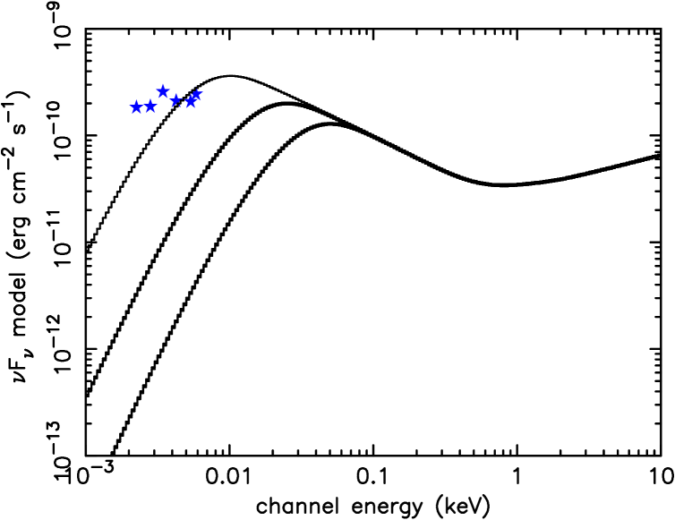
Figure 9: The curves show the extrapolation of the X-ray Comptonisation model down to optical energies for input (disc) temperatures of, from left to right, 2, 5 and 10 eV. The data are taken from revolution 95.

However, it must be noted that 2 eV is far too low a temperature for an accretion disc such as this. Disc theory is still a very uncertain area, especially at high accretion rates. Collin & Huré (2001) and Collin et al. (2002) find that the optical emission in AGN cannot be accounted for by the standard accretion disc model, concluding that, either the disc is ‘non-standard’ or most of the optical luminosity does not come from the accretion disc. A much improved theory of accretion discs is clearly needed, before the relationship between optical and X-ray emission in AGN can be fully understood.

6 Discussion

6.1 3–10 keV band

As mentioned in the introduction (Section 1), 3C 273 has, in the past, shown a hard spectral index of $\sim$ 1.5 (or flatter), while the values found here (Table 3) are noticeably steeper. This is not likely to be due to contamination by the broad soft excess, since the values of $\Gamma$ for the broad-band power-law plus BB fits are very similar to the 3–10 keV slope. Neither does it appear to be a calibration problem, since Molendi & Sembay (2003) also find a relatively steep slope ($\Gamma$ $\sim$ 1.63) for the MECS spectrum over 3–10 keV (SAX data simultaneous with XMM revolution 277).

Using the simple power-law model (Table 3), there is no strong correlation between 3–10 keV $\Gamma$ and the power-law luminosity over the same energy band (Figure 10), with Spearman Rank giving a negligible probability of 9 per cent. However, it is noticeable that the first six observations cluster around a 3–10 keV slope of $\Gamma$ $\sim$ 1.66, while the later three show steeper values, of $\sim$ 1.77.

The open circle in this, and subsequent, plots denotes the data from revolution 472. As mentioned earlier, of the nine observations presented here, it is during revolution 472 that 3C 273 is at its faintest over the 3–10 keV band; revolution 472 is also the shortest of all the observations. Ignoring this data point does not, however, lead to a significant correlation between the 3–10 keV photon index and flux (57 per cent). The relationship between the slope and flux of 3C 273 has been found to vary, however. Agreeing with the present data Turner et al. (1990) found that the parameters were independent, when considering Ginga data between 1983 and 1988; this was also found from RXTE measurements from 1996-1997 (Kataoka et al. 2002). However, from 1999-2000, Kataoka et al. found that the slope became softer when the flux level increased.

Figure 10: If all nine observations are considered, the 3–10 keV photon index is independent of the luminosity over that range. There is a suggestion, however, that 3C 273 exists in two different ‘hardness states’. The open circle represents the revolution 472 data point, while the numbers indicate the chronological order of the measurements.

6.2 Soft excess

6.2.1 0.5-10 keV band

To investigate how the soft excess is changing over time, the Comptonisation model plots for each revolution were overlaid; the result is shown in Figure 11. Above 0.5 keV the fitted spectra show a general tendency for higher flux to be associated with higher temperatures – the hotter the soft excess, the higher the energy the model extends to. Revolution 472 (orange curve) is the exception here, with a high temperature, but a lower normalisation. However, when the model is extrapolated to lower energies, the different $\Gamma$s become more important, the major contribution to the model luminosity being below 0.5 keV and sensitive to the value of $\Gamma$, rather than to kT.

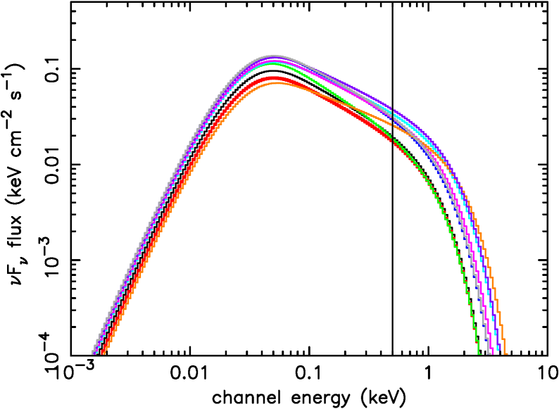
Figure 11: The soft excess of 3C 273 measured during each observation. The vertical line at 0.5 keV shows the point above which the model was fitted; below this energy, the curves are purely an extrapolation. Each revolution is shown in a different colour: black – rev. 94; red – rev. 95; green – rev. 96; blue – rev. 277; light blue – rev. 370; magenta – rev. 373; orange – rev. 472; purple – rev. 554; grey – rev. 563

In order to investigate how the soft excess varies, the parameters ($\Gamma$, optical depth and electron temperature) were plotted against the photon flux calculated over the 0.5–10 keV (observer’s frame) band. Figures LABEL:gamma, 12 and 13 show these results. Spearman Rank (SR) and weighted linear regression were then used to give the probability of a correlation. Linear regression is a useful method, since it takes into account the errors on the measurements, whereas Spearman Rank does not.

An inverse relation is found between the optical depth and the flux over 0.5–10 keV (98 per cent; slope of $-$88 $\pm$ 38) and is shown in Figure 12. Again, excluding the revolution 472 point strengthens the Spearman Rank value, to 99.8 per cent. (The regression slope stays approximately the same, since the point being ignored has relatively large error bars, so would have been less strongly weighted than the other measurements) The other physical parameter of the soft excess – the temperature – shows a 98 per cent positive correlation with the flux (99.8 per cent without revolution 472); that is, the hotter soft excesses are brighter. This is supported by a regression fit of 5.5 $\pm$ 1.3. It must, however, be cautioned that the temperature, kT, and the optical depth, $\tau$, are strongly coupled, as shown by Equations 1 and 2: $\Gamma$ $\sim$ 1/(kT$\tau^{2}$)^1/2.

Figure 12: There is an apparent negative correlation between the optical depth and the flux of the Comptonised soft excess parameter. The open circle represents the revolution 472 data point, as explained in the text.

Figure 13: Over the observed 0.5–10 keV band, when the soft excess is brighter, it is also hotter. The open circle represents the revolution 472 data point.

To try and determine how the regions producing the soft and hard X-rays are linked, Figure 14 was plotted. This shows the fractional (rms) variability of the total observed counts as a function of energy, after the Poisson noise has been accounted for (Edelson et al. 2002) for the MOS data and implies that, over the nine observations, there is very little difference between the rate of variation in the soft and hard bands. The PN results also show that rms variability does not change with energy, although the fraction variability is higher ($\sim$ 32 per cent, compared to $\sim$ 18 per cent in the MOS 2 datasets).

Figure 14: The fractional variabilty amplitude of the MOS 2 data over the nine observations of 3C 273 showing that there is no difference in the variability observed over the different energies. The PN data are consistent with these results.

Figure 15 shows how the two separate Comptonised components vary in flux during the nine observations. It can be seen that the soft excess component varies over a larger range than does the hotter component, although the two generally change in the same sense. This is shown by the standard deviation values of $\sigma$ $\sim$ 0.3 for the range in soft excess variation, compared to $\sigma$ $\sim$ 0.1 for the hotter, power-law component.

Figure 15: Considering the flux of the soft and hard thComp components, the fractional change between revolutions was plotted. In this figure, the solid line joins the soft excess points, while the dashed line joins the ‘power-law’ component values. There is a larger variability in the soft flux, than the hard. The errors on the values are all very small ($<$0.02).

6.2.2 0.001–10 keV band

Cutting the spectrum at 0.5 keV could give a wrong impression of the total luminosity of the soft excess component in the Comptonisation model, since most of the emitted flux is below this energy. For this reason, the optical depth and temperature were plotted against the flux of the extrapolated soft Comptonised component, following the method for investigating the 0.5–10 keV energy band. It must be cautioned, however, that the fluxes and luminosities derived for this extended band are very sensitive to the parameters of the fit.

The correlation between the optical depth and the photon flux (Figure 16) becomes much weaker, with the Spearman Rank probability being 30 per cent for an inverse relation between the two parameters. The kT-flux is also only present at the 30 per cent level, as shown in Figure 17. Neither of these probabilities is significant. If, however, the revolution 472 data point is, again, excluded from the calculation, weak correlations between the photon flux and soft excess temperature or optical depth are revealed (93 per cent, positive/negative for kT/$\tau$ respectively; using linear regression, best-fit slopes of 0.021 $\pm$ 0.006 and $-$0.43 $\pm$ 0.19 are obtained). These correlations are weaker over the full energy band, but are in the same sense as the 0.5–10 keV band.

Figure 16: The open circle represents the revolution 472 data point. If this is excluded, then there is a weak anti-correlation between the optical depth and the photon flux over 0.001–10 keV.

Figure 17: There may be a small, positive correlation between the temperature of the soft excess and the extrapolated photon flux. The open circle represents the revolution 472 data point.

Figures 18 and 19 plot the luminosities and slopes of the two Comptonised components. The soft/hard luminosities appear to be correlated over both bands if weighted linear regression is used to give the line of best fit ($\sim$ 0.14 over both bands); Spearman Rank, however, gives an insignificant result of 74 per cent for the 0.5–10 keV band, though this increases to 96 per cent if the revolution 472 point is ignored. Over 0.001–10 keV, Spearman Rank gives a much larger probability of 99 per cent for a positive correlation (approximately constant with or without revolution 472). The slopes of the cooler and hotter Comptonised components appear to be inversely related, with linear regression giving a slope of $\sim$ $-$1.64, and Spearman Rank giving a (fairly low) probability of 92 per cent for a negative correlation.

Figure 18: There is a positive correlation between the individual Comptonised components, with least squares fitting giving similar slopes of 0.15 $\pm$ 0.03 and 0.13 $\pm$ 0.03 for the 0.5–10 and 0.001–10 keV ranges respectively. The open circle represents the revolution 472 data point.

Figure 19: When fitting the spectra with two Comptonisation components, there is a negative correlation between the values of $\Gamma$: $-$1.64 $\pm$ 0.33. The open circle represents the revolution 472 data point.

6.3 Compton cooling

It is natural to suppose that, if the soft excess were to be produced by Comptonisation of thermal photons from the accretion disc, then an inverse relationship would exist between the photon flux and the electron temperature, caused by Compton cooling. The positive correlation found between kT and the flux over 0.5–10 keV for the soft excess could well have been an artifact of the 0.5 keV cut-off. However, the same sense is observed in the correlation over the full energy band. Thus, the data indicate no negative relationship between the flux and kT and, therefore, no Compton cooling. This implies that the soft excess, if produced by the Comptonisation of thermal disc photons, is more complex than the simple model proposed here. The total soft excess varies from 3.3 $\times$ 10⁴⁶ erg s^-1 up to 6.6 $\times$ 10⁴⁶ erg s^-1, but this is accompanied by a modest increase in temperature. This implies both an increase in the thermal disc emission and a corresponding increase in the electron temperature: two separate mechanisms need to be invoked. Note that the data are inconsistent with a constant photon flux but varying temperature (Figure 17).

7 Conclusions

The XMM spectrum of 3C 273 has been investigated. It is found that the soft X-ray spectrum is dominated by a strong soft excess below $\sim$ 2 keV. This can be well modelled by a multiple blackbody parametrisation, but is most likely to arise though thermal Comptonisation of cool (UV) disc photons in a warm (few hundred eV) corona above the surface of the accretion disc. While the soft excess spectra can be fitted with the Comptonisation model, the variability behaviour is not consistent with a simple interpretation of this model. The temperature of the Comptonising electron cloud may vary independently of the input photon flux, or may even be positively correlated with it. If the latter were to be true, then a further link between the disc emission and the energising of the Comptonising electrons would be necessary.

The individual spectra do not tend to show iron lines, either narrow or broad, neutral or ionised. However, if all the observations are co-added, a weak, broad line is detected.

8 ACKNOWLEDGMENTS

The work in this paper is based on observations with XMM-Newton, an ESA science mission, with instruments and contributions directly funded by ESA and NASA. The authors would like to thank the EPIC Consortium for all their work during the calibration phase, and the SOC and SSC teams for making the observation and analysis possible. This research has made use of the NASA/IPAC Extragalactic Database (NED), which is operated by the Jet Propulsion Laboratory, California Institute of Technology, under contract with the National Aeronautics and Space Administation. Support from a PPARC studentship is gratefully acknowledged by KLP.

References

- [Blaes 2001] Blaes O., Hubeny I., Agol E., Krolik J.H., 2001, ApJ, 563, 560
- [Bowyer 1970] Bowyer C.S., Lampton M., Mack J., de Mendonca F., 1970, ApJ, 161, L1
- [Brinkmann 2001] Brinkmann W. et al. , 2001, A&A, 365, L162
- [Cappi 1998] Cappi M., Matsuoka M., Otani C., Leighly K.M., 1998, PASJ, 50, 213
- [Collin 2001] Collin S., Huré J.-M., 2001, A&A, 372, 50
- [Collin 2002] Collin S., Boisson C., Mouchet M., Dumont A.-M., Coupé S., Porquet D., Rokaki E., 2002, A&A, 388, 771
- [Courvoisier 1987] Courvoisier Th.J.-L. et al. , 1987, A&A, 176, 197
- [Courvoisier 1998] Courvoisier Th.J.-L., 1998, A&ARv, 9, 1
- [den Herder 2001] den Herder J.W. et al. , 2001, A&A, 365, L7
- [Dickey 1990] Dickey J.M., Lockman F.J., 1990, ARA&A, 28, 215
- [Edelson 2002] Edelson R., Turner T.J., Pounds K.A., Vaughan S., Markowitz A., Marshall H., Dobbie P., Warwick R., 2002, ApJ, 568, 610
- [Fang 2003] Fang T., Sembach K.R., Canizares C.R., 2003, ApJ, 586, L49
- [Grandi 1992] Grandi P., Tagliaferri G., Giommi P., Barr P., Palumbo G.G.C., 1992, ApJS, 82, 93
- [Hazard 1963] Hazard C., Mackey M.B., Shimmins A.J., 1963, Nat, 197, 1037
- [Kaspi 2000] Kaspi S., Brandt W.N., Netzer H., Sambruna R., Chartas G., Garmire G.P., Nousek J.A., 2000, ApJ, 535, 17
- [Kataoka 2002] Kataoka J., Tanihata C., Kawai N., Takahara F., Takahashi T., Edwards P.G., Makino F., 2002, MNRAS, 336, 932
- [Kellogg 1971] Kellogg E., Gursky H., Leong C., Schreier E., Tananbaum H., Giaconni R., 1971, ApJ, 165, L49
- [Leach 1995] Leach C.M., McHardy I.M., Papadakis I.E., 1995, MNRAS, 272, 221
- [Lee 2001] Lee J.C., Ogle P.M., Canizares C.R., Marshall H.L., Schulz N.S., Morales R., Fabian A.C., Iwasawa K., 2001, 554, L13
- [Liu 2003] Liu B.F., Mineshige S., Ohsuga K., 2003, ApJ, 587, 571
- [Makishima 1986] Makishima K., Maejima Y., Mitsuda K., Bradt H.V., Remillard R.A., Tuohy I.R., Hoshi R., Nakagawa M., 1986, ApJ, 308, 635
- [Marshall 1995] Marshall H.L., Fruscione A., Carone T.E., 1995, ApJ, 439, 90
- [Mason 2001] Mason K.O. et al. , 2001, A&A, 365, L36
- [Mitsuda 1984] Mitsuda K. et al. , 1984, PASJ, 36, 741
- [Molendi 2002] Molendi S., Sembay S., 2003, EPIC technical note, XMM-SOC-CAL-TN-0036
- [Nandra 1997] Nandra K., George I.M., Mushotsky R.F., Turner T.J., Yaqoob T., 1997, ApJ, 488, L91
- [O’Brien 2001] O’Brien P.T., Page K., Reeves J.N., Pounds K., Turner M.J.L., Puchnarewicz E.M., 2001, MNRAS, 327, L37
- [Orr 1998] Orr A., Yaqoob T., Parmar A.N., Piro L., White N.E., Grandi P., 1998, A&A, 337, 685
- [Page 2003] Page K.L., O’Brien P.T., Reeves J.N., Turner M.J.L., 2003, MNRAS, in press (astro-ph/0309394)
- [Rasmussen 2003] Rasmussen A., Kahn S.M., Paerels F., 2003, in ‘The IGM/Galaxy connection: The distribution of baryons at z = 0’, Kluwer Academic Publishing (astro-ph/0301183)
- [Sako 2001] Sako M. et al. , 2001, A&A, 365, L168
- [Saxton 1993] Saxton R.D., Turner M.J.L., Williams O.R., Stewart G.C., Ohashi T., Kii T., 1993, MNRAS, 262, 63
- [Schmidt 1963] Schmidt M., 1963, Nat, 197, 1040
- [Staubert 1992] Staubert R., 1992, in X-ray Emission from AGN and the Cosmic X-ray background, ed. W. Brinkmann, J. Trümper, MPE Rep. 235, 42
- [Strüder 2001] Strüder L. et al. , 2001, A&A, 365, L18
- [Sunyaev 1980] Sunyaev R.A., Titarchuk L.G., 1980, A&A, 86, 121
- [Turner 1985] Turner M.J.L., Courvoisier Th., Staubert R., Molteni D., Trümper J., 1985, in Proc. of 18th ESLAB Symp., ed. A. Peacock, Reidel, Dordrecht, 623
- [Turner 1990] Turner M.J.L. et al. , 1990, MNRAS, 244, 310
- [Turner 1991] Turner T.J., Weaver K.A., Mushotzky R.F., Holt S.S., Madejski G.M., 1991, ApJ, 381, 85
- [Turner 2001] Turner M.J.L. et al. 2001, A&A, 365, L27
- [Wilkes 1987] Wilkes B.J., Elvis M., 1987, ApJ, 323, 243
- [Williams 1992] Williams O.R. et al. , 1992, ApJ, 389, 157
- [Yaqoob 2000] Yaqoob T., Serlemitsos P., 2000, ApJ, 544, L95
- [Yaqoob 1994] Yaqoob T. et al. , 1994, PASJ, 46, L49
- [Zycki 1999] Życki P.T., Done C., Smith D.A., 1999, MNRAS, 305, 231