FAINT 6.7 $\mu$m GALAXIES AND THEIR CONTRIBUTIONS TO THE STELLAR MASS DENSITY IN THE UNIVERSE

Abstract

We discuss the nature of faint 6.7 $\mu$m galaxies detected with the mid-infrared camera ISOCAM on board the Infrared Space Observatory (ISO). The 23 hour integration on the Hawaii Deep Field SSA13 has provided a sample of 65 sources down to 6 $\mu$Jy at 6.7 $\mu$m. For 57 sources, optical or near-infrared counterparts were found with a statistical method. All four Chandra sources, three SCUBA sources, and one VLA/FIRST source in this field were detected at 6.7 $\mu$m with high significance. Using their optical to mid-infrared colors, we divided the 6.7 $\mu$m sample into three categories: low redshift galaxies with past histories of rapid star formation, high redshift ancestors of these, and other star forming galaxies. Rapidly star forming systems at high redshifts dominate the faintest end. Spectroscopically calibrated photometric redshifts were derived from fits to a limited set of template SEDs. They show a high redshift tail in their distribution with faint ($<30$ $\mu$Jy) galaxies at $z>1$. The 6.7 $\mu$m galaxies tend to have brighter $K$ magnitudes and redder $I-K$ colors than the blue dwarf population at intermediate redshifts. Stellar masses of the 6.7 $\mu$m galaxies were estimated from their rest-frame near-infrared luminosities. Massive galaxies ($M_{\mathrm{star}}\sim 10^{11}$ M_⊙) were found in the redshift range of $z=0.2$–3. Epoch dependent stellar mass functions indicate a decline of massive galaxies’ comoving space densities with redshift. Even with such a decrease, the contributions of the 6.7 $\mu$m galaxies to the stellar mass density in the universe are found to be comparable to those expected from UV bright galaxies detected in deep optical surveys.

1. INTRODUCTION

The evolution of galaxies can be traced in their spectral energy distributions (SEDs) as a result of the aging and accumulation of stellar populations. Because more massive stars evolve faster, ultraviolet (UV) emission becomes relatively weaker as time elapses, provided that no further star formation occurs. This sensitivity to on-going star formation can be used to trace the star formation history in galaxies; however, the UV light suffers from dust extinction. Thus, optical observations of the redshifted UV emission from distant galaxies need undesirable corrections if we are to deduce the evolution of their star forming activity.

However, if we observe galaxies at a longer wavelength, this undesirable situation is improved. At rest near-infrared wavelengths, much of the emission originates from low mass stars. Their lifetime is comparable to the age of the universe; thus, the effect of aging is much milder than that in the UV. The complicating effects of dust extinction are almost negligible at this wavelength. Most of the changes in the near-infrared SEDs are caused by the accumulation of stellar populations in galaxies. These facts assure good accuracy in estimating stellar masses of galaxies from their near-infrared luminosities.

The stellar mass is one of the most fundamental quantities of galaxies. This motivates the execution of galaxy surveys in the near-infrared. For distant galaxies, very sensitive surveys should be performed at a longer wavelength in order to detect their rest-frame near-infrared light. The mid-infrared camera ISOCAM (Cesarsky et al., 1996) on board the Infrared Space Observatory (ISO, Kessler et al., 1996) has achieved such requirements for the first time.

Most of the deep ISOCAM surveys have utilized two broad band filters: LW2 (5–8.5 $\mu$m) at 6.7 $\mu$m and LW3 (12–18 $\mu$m) at 15 $\mu$m (Serjeant et al., 1997; Taniguchi et al., 1997; Flores et al., 1999a, b; Altieri et al., 1999; Oliver et al., 2002). In particular, those at 15 $\mu$m attracted much interest (Genzel & Cesarsky, 2000; Franceschini et al., 2001, 2003), mainly due to the discovery of a strongly evolving population of galaxies below 1 mJy (Elbaz et al., 1999). The excess in number could be explained by a large number of star forming galaxies at $z\sim 1$.

The 6.7 $\mu$m cosmological observations with ISOCAM resulted in generally fewer detections than at 15 $\mu$m and thus attracted less attention. This is because such observations should sample a wavelength valley in galaxy SEDs between stellar and hot dust emission. The passband of the LW2 filter matches the location of the unidentified infrared band (UIB) emission in the local universe. Such dust emission shifts away from the passband with redshift (Aussel et al., 1999). At high redshifts $z>1$, the major contribution to the LW2 band becomes stellar emission in galaxies. However, such emission from distant galaxies requires extremely high sensitivities. Based on the importance of detecting near-infrared stellar emission from high redshift galaxies for estimating their stellar masses, we conducted a very deep 6.7 $\mu$m survey in the Hawaii Deep Field SSA13 (Sato et al., 2003). One sigma sensitivity reached 3 $\mu$Jy, which is smaller than the published values of 7 $\mu$Jy in Taniguchi et al. (1997) and in Aussel et al. (1999). Most recently, Metcalfe et al. (2003) reach a depth similar to ours using a massive cluster lens. In this paper, we discuss insights deduced from the faint 6.7 $\mu$m galaxies detected in the SSA13 field.

After describing the 6.7 $\mu$m sample in Sect. 2, we discuss the identification of multi-wavelength counterparts (Sect. 3). In Sect. 4, the nature of the identified galaxies is examined with the GRASIL star/dust SED model (Silva et al., 1998). Their stellar masses are obtained using the rest-frame near-infrared luminosities, and then we discuss the evolution of the stellar mass function and the stellar mass density in the universe (Sect. 5). Finally, we present a discussion (Sect. 6) and conclusions (Sect. 7). Throughout this paper, we assume a flat universe with $\Omega_{\mathrm{M}}=0.3$, $\Omega_{\Lambda}=0.7$, and $H_{0}=65\,\mathrm{km}\,\mathrm{s}^{-1}\,\mathrm{Mpc}^{-1}$. All optical and near-infrared magnitudes in this paper are in the Vega system.

2. THE 6.7 $\mu$m SAMPLE

A deep mid-infrared survey has been conducted with the ISOCAM array on board the Infrared Space Observatory (ISO). The broadband filter LW2 (5–8.5 $\mu$m) with the reference wavelength of 6.7 $\mu$m was used to image a high galactic latitude region in the Hawaii Deep Field SSA13. Many raster observations totaling an observing time of 23 hours were combined to give a map with a nominal areal coverage of 16 arcmin² with the beam FWHM of 7.2 arcsec. Details of the observations are given in Sato et al. (2003).

With a non-uniform noise distribution over the map, source detections were performed using a signal-to-noise ratio (S/N) map. The noise map was created from the standard deviations of the co-added raster images at each pixel. Detection parameters were determined by comparing numbers of detected sources at the positive and negative sides of the map ($N_{\mathrm{pos}}$ and $N_{\mathrm{neg}}$, respectively) with the same detection parameter set. We have chosen the parameter set giving the largest $N_{\mathrm{pos}}-N_{\mathrm{neg}}$, where $N_{\mathrm{pos}}=65$ and $N_{\mathrm{neg}}=12$. Total 6.7 $\mu$m fluxes of the positive sources resulted in a range from 6 $\mu$Jy to 170 $\mu$Jy (Table FAINT 6.7 $\mu$m GALAXIES AND THEIR CONTRIBUTIONS TO THE STELLAR MASS DENSITY IN THE UNIVERSE).

By setting a threshold that can exclude all the negative sources, we extracted a subsample of the positive sources. This subsample, the primary sample, consists of 33 sources having total fluxes larger than 12 $\mu$Jy and detection S/Ns larger than 4.3 (Table FAINT 6.7 $\mu$m GALAXIES AND THEIR CONTRIBUTIONS TO THE STELLAR MASS DENSITY IN THE UNIVERSE). Because there should be no effects from spurious detections in the primary sample, our main results will be deduced based on the primary sample. No corrections for the contamination of fake sources are necessary for the primary sample to derive integrated quantities such as stellar mass functions and stellar mass densities discussed in Sect. 5. In fact, galaxy number counts shown in Sato et al. (2003) were obtained only with the primary sample.

The remaining 32 positive sources are put into the supplementary sample. For the number of negative sources ($N_{\mathrm{neg}}=12$) having comparably low significance values, the number of true sources in the supplementary sample could be 20. However, we expect more sources in the supplementary sample are real. This is because the adopted image processing could produce negative ghosts around bright sources, and at least three of the negative sources were identified as such (Sato et al., 2003). Genuine sources in the supplementary sample should provide meaningful information on the 6.7 $\mu$m sources, especially at the faintest flux levels. Some of them will be mentioned in the following sections with a caveat that there will be some effects from spurious sources.

In Table FAINT 6.7 $\mu$m GALAXIES AND THEIR CONTRIBUTIONS TO THE STELLAR MASS DENSITY IN THE UNIVERSE, sources in both samples are listed. Here we also show the 12 negative sources as the negative sample. All are to be examined with the source identification procedure in the next section.

3. SOURCE IDENTIFICATION

Counterparts of the 6.7 $\mu$m sources were searched at multiple wavelengths, from the X-ray to the radio. We used two identification methods, the probability ratio method in the optical and near-infrared, and the nearest neighbor search at X-ray, submillimeter, and radio wavelengths. The results are summarized in two tables, Tables FAINT 6.7 $\mu$m GALAXIES AND THEIR CONTRIBUTIONS TO THE STELLAR MASS DENSITY IN THE UNIVERSE and FAINT 6.7 $\mu$m GALAXIES AND THEIR CONTRIBUTIONS TO THE STELLAR MASS DENSITY IN THE UNIVERSE, respectively.

3.1. Optical and Near-Infrared Identifications

3.1.1 The identification procedure

Optical and near-infrared counterparts of the 6.7 $\mu$m sources were sought in the $K$, $I$, and $B$ bands. These three band data were taken from the ground (Cowie et al., 1996), but we utilized a $HST$/WFPC2 catalogue in the $I_{814}$ band as well (Cowie, Hu, & Songaila, 1995). The catalogue limits were estimated as $K=19.9$, $I_{814}=24.7$, $I=23.7$, and $B=25.5$ (3 $\sigma$). Photometric uncertainties were derived by summing relative and absolute uncertainties quadratically. Absolute photometric uncertainties were estimated to be 0.1 magnitude for corrected aperture magnitudes (Cowie et al., 1994). We do not distinguish between $I_{814}$ and $I$ magnitudes in the following, because these magnitudes for the same sources in our sample do not show significant differences. At these magnitude limits, surface densities become higher than that of the 6.7 $\mu$m sources. We then introduced the following two probabilities to evaluate whether a candidate counterpart of magnitude $m_{1}$ at distance $r_{1}$ should be considered as a true association (Mann et al., 1997; Flores et al., 1999a).

Even for a true association between sources at two wavelengths, there is expected to be a certain amount of displacement in their positions. If we can neglect differences in light profiles at the two wavelengths, a major cause for the displacement will be measurement errors at both wavelengths. Based on smaller beam sizes in the optical and near-infrared ($\sim 1$ arcsec or less), we only took account of measurement errors in the 6.7 $\mu$m coordinates. With an assumption that the errors follow a Gaussian distribution, the probability for a true association $P_{\mathrm{t}}$ is defined as

$$P_{\mathrm{t}}=1-\sqrt{\frac{2}{\pi}}\int_{0}^{\alpha}\exp(-\frac{x^{2}}{2})dx,$$ (1)

where $\alpha(=r_{1}/r_{0})$ is the displacement of a potential counterpart normalized to the one sigma positional accuracy $r_{0}$ of the 6.7 $\mu$m source in question. This $r_{0}$ value was determined with Monte-Carlo simulations in Sato et al. (2003).

As long as the displacement has a finite value $r_{1}$, we can not exclude the possibility that an irrelevant source will be found at a distance smaller than $r_{1}$. Such a chance event should follow Poisson statistics for an area of ${\pi}{r_{1}}^{2}$. Then the probability for a chance association $P_{\mathrm{c}}$ is derived as

$$P_{\mathrm{c}}=1-\exp(-{\pi}{r_{1}}^{2}N(<{m_{1}})),$$ (2)

where $N(<{m_{1}})$ is the surface density of optical or near-infrared sources with magnitudes brighter than $m_{1}$, the magnitude of a potential counterpart. Because only two stars are expected in this 6.7 $\mu$m sample (Sato et al., 2003), $N(<m)$ was derived by integrating differential galaxy counts shown in Metcalfe et al. (2001) and in Maihara et al. (2001).

These two probabilities, $P_{\mathrm{t}}$ and $P_{\mathrm{c}}$, were calculated for all potential counterparts up to a distance of $3\,r_{0}$ from each 6.7 $\mu$m position. The large search radius was necessary to take account of the large uncertainty in the determination of $r_{0}$ (Sato et al., 2003). We then selected an optical or near-infrared counterpart having the highest ratio of $P_{\mathrm{t}}/P_{\mathrm{c}}$. If there is no candidate source with $P_{\mathrm{t}}/P_{\mathrm{c}}>1$, the 6.7 $\mu$m source was regarded as unidentified. Assuming that SEDs of the 6.7 $\mu$m sources are smoothly connected, we performed the identification procedure starting from the nearest wavelength. The adopted $K$ and $I_{814}$ band catalogues do not cover the full 6.7 $\mu$m field. Taking also account of the deeper limit for the $I_{814}$ band catalogue, the identification scheme was then set from the $K$, $I_{814}$, $I$, to $B$ band. If the identification at a particular band resulted in a success, counterparts at the shorter wavelengths were found with a nearest neighbor search. A search up to 1.4 arcsec for it turned out to be enough.

3.1.2 Identification results

Of 65 positive sources, 57 were identified in the optical or near-infrared. Fig. 1 shows their appearances at the wavelength where the probability calculations were performed. In Table FAINT 6.7 $\mu$m GALAXIES AND THEIR CONTRIBUTIONS TO THE STELLAR MASS DENSITY IN THE UNIVERSE, identification band (ID), distance ($r_{1}$), two probabilities ($P_{\mathrm{t}}$ and $P_{\mathrm{c}}$), and their ratio are listed. The coordinates of the identified sources have been updated with those of the optical or near-infrared counterparts. We also show the second highest ratio of $P_{\mathrm{t}}/P_{\mathrm{c}}$ ($P_{\mathrm{t}}/P_{\mathrm{c}}^{(2)}$) if other candidates were found in the search radius. There are relatively few cases of ambiguous identifications (i.e., where the second largest $P_{\mathrm{t}}/P_{\mathrm{c}}$ is of the same order of magnitude as the largest). In particular, in the primary sample, only one source (#59) seems to fall in this category. In the following, the identification results for the primary and supplementary samples are examined separately.

For the primary sample, we found that many sources were identified in the $K$ band. All the sources that were identified at shorter wavelengths have large $P_{\mathrm{t}}/P_{\mathrm{c}}$ values. As indicated in Table FAINT 6.7 $\mu$m GALAXIES AND THEIR CONTRIBUTIONS TO THE STELLAR MASS DENSITY IN THE UNIVERSE, they either lack $K$ data (#30, #39, and #62) or have blue colors (#44 and #64). Sato et al. (2002) identified the source #40 with a submillimeter source with a hard X-ray counterpart. This identified source has a smaller significance value ($P_{\mathrm{t}}/P_{\mathrm{c}}\sim 0.6$) than the nominal threshold ($P_{\mathrm{t}}/P_{\mathrm{c}}=1$) at the $K$ band. We regard it as likely that the asymmetric profile of this 6.7 $\mu$m source (Sato et al., 2002) affected the probability calculation. The only unidentified source #27, having a high S/N=10, lacks $K$ data (Table FAINT 6.7 $\mu$m GALAXIES AND THEIR CONTRIBUTIONS TO THE STELLAR MASS DENSITY IN THE UNIVERSE) and has a very red mid-infrared to optical color.

The lower significance of the supplementary sample leads to poorer positional accuracy ($r_{0}\sim$ 2–3 arcsec), which made the identification more difficult. Even in such circumstances, 78 % (25/32) of the supplementary sample were identified. Because the supplementary and negative samples have the same S/N level, the identification significance for the supplementary sample can be checked by a comparison with the negative sample. No source in the negative sample was identified in the $K$ band. Thus the identifications of the supplementary sample in the $K$ band are expected to be robust. Three sources in the negative sample were identified in the $I$ or $I_{814}$ band. However, most of the $I$ or $I_{814}$ band identifications in the supplementary sample have better statistics, i.e, larger $P_{\mathrm{t}}/P_{\mathrm{c}}$ values than those for the $I$ or $I_{814}$ band identifications in the negative sample. Here $I$ and $I_{814}$ counterparts should be treated separately because of the difference in the catalogue depth. The deeper $I_{814}$ sources generally have smaller $P_{\mathrm{t}}/P_{\mathrm{c}}$ values due to the larger surface density of sources. The $I_{814}$ counterparts for sources #21 and #24 have larger $P_{\mathrm{t}}/P_{\mathrm{c}}$ values than that of the $I_{814}$ counterpart for the negative source N7. The $I$ counterparts for sources #12, #29, #34, #46, #58, and #60 have larger $P_{\mathrm{t}}/P_{\mathrm{c}}$ values than that of the $I$ counterpart for the negative source N9, which has a $P_{\mathrm{t}}/P_{\mathrm{c}}$ value larger than N10. The remaining $I$ or $I_{814}$ band identifications are for sources #2, #31, #43, and #52, though most of them have slightly smaller $P_{\mathrm{t}}/P_{\mathrm{c}}$ values than that of their corresponding negative source: N7 or N9. Thus, we expect the number of erroneous identifications in the supplementary sample will be quite small, four at most. The number of unidentified sources in the supplementary sample (7) is comparable to that in the negative sample (9). This indicates that some of the unidentified sources in the supplementary sample could be spurious, especially those detected in noisy regions of the map (e.g. sources #7 and #37). However, some could be very red sources like the source #27 in the primary sample.

Flores et al. (1999a) give $r_{1}$ and $P_{\mathrm{c}}$ values for the identification of their 6.7 $\mu$m sources. Their values are generally larger than ours; the median $r_{1}$ is 4.2 arcsec and $P_{\mathrm{c}}$ exceeds 0.3 in some cases. We think that this may be partly due to their neglect of distortion corrections in data processing, which could be as large as one 6 arcsec pixel in size. They adopted 1.5 arcsec map pixels and used only 3–5 sources to determine shifts between images. The median FWHM of 6.7 $\mu$m sources on their final map was 11 arcsec, while ours was 7.2 arcsec. We took account of distortion corrections and used 0.6 arcsec map pixels and 19 reference sources for the image registration (Sato et al., 2003). The difference mentioned above might not explain all of the difference in their identification results. Rather, even the sources identified with the least significance in Flores et al. (1999a) have 6.7 $\mu$m fluxes larger than ours and correspondingly optical magnitudes brighter than ours.

3.2. X-ray, Submillimeter, and Radio Identifications

At the flux levels of the adopted X-ray, submillimeter, and radio catalogues, the surface densities are lower than that of our mid-infrared sample. Thus, source identification at these wavelengths can be achieved using a simple method, a nearest neighbor search.

With the deep Chandra observations of SSA13 (Mushotzky et al., 2000), four X-ray sources were detected within the area of the ISOCAM survey. Three of them were detected in the hard X-ray band (2–10 keV) with fluxes larger than $4\times 10^{-15}\mathrm{erg}\,\mathrm{s}^{-1}\,\mathrm{cm}^{-2}$, while two of them were detected in the soft X-ray band (0.5–2 keV) with fluxes larger than $8\times 10^{-16}\mathrm{erg}\,\mathrm{s}^{-1}\,\mathrm{cm}^{-2}$ (Table FAINT 6.7 $\mu$m GALAXIES AND THEIR CONTRIBUTIONS TO THE STELLAR MASS DENSITY IN THE UNIVERSE). Within 1.1 arcsec of these four X-ray sources, comparable to the positional accuracy of the Chandra satellite, we found 6.7 $\mu$m counterparts #14, #17, #40 and #62. Here we have used the 6.7 $\mu$m coordinates updated with the optical and near-infrared identifications above.

The Submillimetre Common-User Bolometer Array (SCUBA) on the 15 m James Clerk Maxwell Telescope (JCMT) detected three 850 $\mu$m sources down to 2 mJy in the deep SCUBA survey of SSA13 (Barger et al., 1999). Taking account of the very broad beam at 850 $\mu$m (15 arcsec FWHM), all the three submillimeter sources were identified with 6.7 $\mu$m sources #28, #40, and #57 at distances of up to 7.7 arcsec (Sato et al., 2002). Note that one of the submillimeter sources (#40) was also detected in the hard X-ray.

The VLA/FIRST survey at 1.4 GHz detected one 3 mJy source in the 6.7 $\mu$m SSA13 map (White et al., 1997). This source is also listed in the VLA/NVSS catalogue (Condon et al., 1998). The 6.7 $\mu$m counterpart is assigned to the source #20 at a distance of 0.2 arcsec.

All these X-ray, submillimeter, and radio sources are in the primary sample. Except for one optically bright hard X-ray source #62, the others have 6.7 $\mu$m fluxes in a range of 10–30 $\mu$Jy.

4. THE NATURE OF FAINT 6.7 $\mu$m GALAXIES

We have identified two stars in the 6.7 $\mu$m sample using their image profiles in the optical (Sato et al., 2003). Excluding these stars from the primary sample, we now discuss the nature of the remaining sources, all of which are assumed to be galaxies. We utilize the GRASIL star/dust galaxy SED model (Silva et al., 1998), which is explained in some detail in Appendix A.

4.1. Colors

With the $K$, $I$, and $B$ band photometry, we examined the distributions of faint 6.7 $\mu$m galaxies in various color-color plots. In one plot (Fig. 2), we identified a distinct population of faint 6.7 $\mu$m galaxies having red $B-I$ colors and low ratios of $f_{\nu}(6.7\mu\mathrm{m})/f_{\nu}(K)$. To derive ratios with 6.7 $\mu$m fluxes, we used zero-point fluxes of 645 Jy, 2408 Jy, and 3974 Jy for $K$, $I$, and $B$ magnitudes, respectively. Solid circles with error bars show sources in the primary sample. Empty circles are for the supplementary sources. Color limits using 3 $\sigma$ magnitude limits or real measurements for saturated sources or for sources at the image boundaries are indicated with arrows. Some sources are not shown due to lack of information, such as no data in the $K$ band, or no detections in both $I$ and $B$ bands. The concentration of galaxies at the upper-left part of the panel is distinct from the rest of the sample by more than the relatively large errors in $f_{\nu}(6.7\mu\mathrm{m})/f_{\nu}(K)$ ratios. We assigned an identification flag of type I for galaxies in this concentration (Table FAINT 6.7 $\mu$m GALAXIES AND THEIR CONTRIBUTIONS TO THE STELLAR MASS DENSITY IN THE UNIVERSE). The type I galaxies are marked with squares and can be separated from the rest of the galaxies with the dot-dashed line in the plot.

On the same panel, we overlaid some model predictions using the GRASIL SEDs (Appendix A). The evolving SEDs for three $z=0$ Hubble types – E, Sa, and Sc galaxies – are shown with dashed, dotted, and solid lines, respectively. For each Hubble type, we assumed three formation redshifts of $z_{\mathrm{f}}=2$, 3, and 10 (thick, medium, and thin lines, respectively). The locations of $z=0$ galaxies are shown with solid triangles, while $z=1$, 2, and 3 with empty triangles (for $z<z_{\rm f}$). We find that type I galaxies follow lines for the evolving E galaxies at intermediate redshifts of $z=0$–1, regardless of their assumed formation redshifts. The evolving Sa galaxy predictions also share the same region, but higher formation redshifts are preferred. In our adopted cosmology, the ages of galaxies with $z_{\mathrm{f}}=2$, 3, and 10 at $z=1$ become 2.5 Gyr, 3.6 Gyr, and 5.3 Gyr, respectively. This indicates that type I galaxies would be old and matured systems whose stellar contents are already in place as a consequence of vigorous star formation a long time ago (see Fig. 14).

The other galaxies in this plot follow the GRASIL predictions; however, almost nothing can be drawn from this figure because of the degeneracy of the model loci. Both rapidly star-forming galaxies at high redshifts and quiescently star-forming galaxies show high ratios of $f_{\nu}(6.7\mu\mathrm{m})/f_{\nu}(K)$ and blue $B-I$ colors. The color degeneracy in this part of the plot can be disentangled to some degree by changing color combinations. In Fig. 3, we show $f_{\nu}(6.7\mu\mathrm{m})/f_{\nu}(I)$ ratios and $B-K$ colors. In this plot, the evolving E or Sa galaxies can be red in both colors, while the evolving Sc galaxies occupy the lower left part of the panel with blue $B-K$ colors and low ratios of $f_{\nu}(6.7\mu\mathrm{m})/f_{\nu}(I)$. The evolving E and Sa galaxies with lower formation redshifts ($z_{\mathrm{f}}<3$) can have such blue colors at their forming stage ($z\sim z_{\mathrm{f}}$). Thus, these blue colors can be an indicator of on-going star formation.

The distribution of the 6.7 $\mu$m galaxies in this plot is rather smooth, except for the type I galaxies marked with squares. However, we here introduced a separation line (dot-dashed line) to extract many sources not detected in the $B$ band. These can be explained as high redshift galaxies ($z>1$) with rapid star forming activities at the past (evolving E or Sa galaxies). They represent post-starburst galaxies at high redshift. Their properties are consistent with those of ancestors of type I galaxies. We here categorize them as type II and mark them with diamonds. The remaining galaxies are assigned as type III. They are on-going star formers at $z=0$–2, a combination of mildly star forming galaxies and vigorously star forming galaxies with low formation redshifts.

The division of the sources into types I, II, and III is made in color-color plots with photometry in all four bands – 6.7 $\mu$m, $K$, $I$ and $B$. We find that this division can also be applied to the color-color plot of $f_{\nu}(6.7\mu\mathrm{m})/f_{\nu}(I)$ vs $f_{\nu}(6.7\mu\mathrm{m})/f_{\nu}(B)$. In this plot, we can assign type identifiers to all the 6.7 $\mu$m sources, with the help of the distribution of the sources whose types have been defined in the previous two plots. Even unidentified sources could have a nominal type of II by their red colors due to their flux limits at the $I$ and $B$ bands. For the primary sample, the number ratio for the 31 galaxies becomes type $\mathrm{I}:\mathrm{II}:\mathrm{III}=11:10:10$ including the unidentified source #27 with type II (Table FAINT 6.7 $\mu$m GALAXIES AND THEIR CONTRIBUTIONS TO THE STELLAR MASS DENSITY IN THE UNIVERSE). This almost even distribution skews toward the dominance of type II in the supplementary sample. For the 32 sources in this sample, the ratio becomes type $\mathrm{I}:\mathrm{II}:\mathrm{III}=5:23:4$. The dominance of type II in this fainter sample is still valid even if the seven unidentified sources assigned type II are excluded.

4.2. Redshifts

In order to obtain absolute quantities such as stellar masses for the 6.7 $\mu$m galaxies, we need their redshifts. For the 55 identified 6.7 $\mu$m galaxies, we do have 21 spectroscopic redshifts $z_{\mathrm{sp}}$, of which 18 are for the primary sample (Songaila et al., 1994; Cowie et al., 1996; Barger et al., 2001). For others, we derived photometric redshifts $z_{\mathrm{ph}}$ in the following way.

4.2.1 Photometric redshifts

Photometric redshifts were estimated by minimizing $\chi^{2}$ values between photometric measurements and model estimates. This is basically the same method adopted in the the $hyperz$ code by Bolzonella, Miralles, & Pelló (2000). We used 6.7 $\mu$m, $K$, $I$, and $B$ band fluxes or their limits listed in Table FAINT 6.7 $\mu$m GALAXIES AND THEIR CONTRIBUTIONS TO THE STELLAR MASS DENSITY IN THE UNIVERSE. For sources in Table FAINT 6.7 $\mu$m GALAXIES AND THEIR CONTRIBUTIONS TO THE STELLAR MASS DENSITY IN THE UNIVERSE, we tried to utilize their flux values or their limits at the X-ray, submillimeter, and radio wavelengths as well. Model estimates were obtained using two sets of the star/dust SEDs in the GRASIL library; the evolving SEDs and the local ones (Appendix A). We also added two SEDs expanded to the X-ray wavelengths; a NGC 6240 SED compiled by Hasinger (2000) and a GRASIL Arp220 SED complemented with X-ray and radio observations (Iwasawa, 1999; Carilli & Yun, 2000).

The $\chi^{2}$ minimization was executed SED by SED in our code. The SEDs used have a long wavelength baseline; the GRASIL local SEDs from UV to submillimeter, the GRASIL evolving SEDs from UV to radio, and the two additional SEDs from X-ray to radio. They are likely to have significance variations at different wavelengths; however, we neglected such errors in the SEDs. We thus considered noise only in the absolute photometric measurements. For each SED, we calculated $\chi^{2}$ values at 100 redshifts from $z=0.1$ to 10. The interval of the redshift grid was constant in $\log(1+z)$. Once the redshift giving the minimum $\chi^{2}$ value was derived, we repeated the calculation around this redshift with a ten times finer redshift resolution. After completing the $\chi^{2}$ minimization for all the SEDs, we determined a photometric redshift giving the minimum $\chi^{2}$ value among the SEDs. We also found that in most cases, the redshift giving the minimum $\chi^{2}$ value for each SED is consistent with the photometric redshift determined by the global minimum in $\chi^{2}$. It should be noted that the final photometric redshifts were all determined with the UV-to-submillimeter SEDs because the SEDs expanded to the radio and/or X-ray resulted in high $\chi^{2}$ values. For the comparison of $\chi^{2}$ values among SEDs with different wavelength spans, we took proper account of both the values of $\chi^{2}$ and the number of the detected data points used to calculate $\chi^{2}$. In these calculations, we did not require that the age of the SED template be less than the age of the universe at a given redshift. Previous works on photometric redshifts have given good results with local templates at high redshifts (see e.g., Hogg et al., 1998). We therefore tried to fit local SEDs even at $z=10$. Old evolving SEDs were also treated as local SEDs. This assures a possible range of SED variations. Actually, we found that the results of this approach admitting the age-inconsistency in the fits gave the best results in the comparison with spectroscopic redshifts explained below.

We show some fitting results at different redshifts in Fig. 4. Photometric redshifts and their 90 % confidence limits (Avni, 1976) are listed in Table FAINT 6.7 $\mu$m GALAXIES AND THEIR CONTRIBUTIONS TO THE STELLAR MASS DENSITY IN THE UNIVERSE. The names of the best-fit SEDs, their $\chi^{2}$ values, and some ancillary information of the fits are also shown. It should be noted that many other SEDs gave quite similar redshift estimates with somewhat larger $\chi^{2}$ values. For source #38, which has the largest $\chi^{2}$ value in the sample, 12 SEDs gave $z=0.74$–0.98 with $\chi^{2}=9.9$–15. On the other hand, many sources have $\chi^{2}=0.0$, though they are truncated values. This indicates overestimates of our photometric errors. This is likely in our case due to quadratic summation of error components, each of which was difficult to determine independently. Our data points are very sparse in wavelength. In a sense, we might have used too many sets of SEDs for such data sets. It can be said that we have allowed the SEDs to shift freely in redshift space to take account of the symmetric distribution of photometric errors. We have succeeded in eliminating outlier fits; however, some fits could have fallen at rather artificial $\chi^{2}$ minima. Thus, the confidential intervals are more reliable than photometric redshift values themselves. It should be noted that the photometric redshift determination technique basically utilizes the characteristic spectral features common to all SEDs. There is some information in the fit; however, the very particular SED names identified as giving the best photometric redshifts do not exclude other SED types.

The reliability of these redshift estimates can be addressed by computing photometric redshifts for sources with spectroscopic redshifts. The results are shown in Fig. 5. Of 21 sources with spectroscopic redshifts, 10 photometric redshifts were derived with the age-inconsistent evolving SEDs, 6 with local templates, and 5 with age-consistent SEDs. This result assures the usefulness of the admittance of age-inconsistency in the fits. Actually, most of the photometric estimates follow the identity relation with their spectroscopic measurements. The nominal dispersion was 0.2 dex in $\log z$ (dotted lines). Only four sources, #62, #15, #29, and #16 with spectroscopic redshifts of $z\sim 0.2$, 0.3, 0.6, and 1.2, respectively, gave photometric redshifts larger by more than one sigma. However, their large 90 % confidence intervals indicate that they are essentially problematic data sets. For example, source #62 lacks any flux constraint in the $K$ band.

The four photometric bands, $B$, $I$, $K$, and 6.7 $\mu$m, are widely and evenly distributed in wavelength (Fig. 4). The determination of photometric redshifts with these data sets appears to depend on a characteristic spectral peak around 1.6 $\mu$m corresponding to the H^- opacity minimum for the stellar continuum emission. The use of this 1.6 $\mu$m bump for photometric redshifts with photometric data sets without wavelength gaps is described in Sawicki (2002). In wider wavelengths, the spectral slope is generally monotonic below 1.6 $\mu$m, while there could be UIB emission longward of the 1.6 $\mu$m peak until 6.7 $\mu$m (i.e. 3.3 $\mu$m and 6.2 $\mu$m). There is a possibility that some UIB emission was erroneously treated as a shorter wavelength feature. Misidentification of 6.2 $\mu$m emission with a 3.3 $\mu$m or 1.6 $\mu$m feature gives a wrong redshift of $z\sim 1$ or 3 and that of 3.3 $\mu$m emission with a 1.6 $\mu$m feature gives $z\sim 1$. Unfortunately, the 6.7 $\mu$m photometric band is very broad (5–8.5 $\mu$m) and the gaps between the four photometric bands are somewhat large. Some sources are even lacking some of the four flux values. This all could give a reason for the four high redshift outliers in Fig. 5. The effects of $z_{\rm ph}>z_{\rm sp}$ estimates will be addressed in the following sections.

4.2.2 Fluxes and redshifts

With redshifts determined spectroscopically or photometrically, 6.7 $\mu$m fluxes for all 55 identified galaxies are plotted as a function of redshift in Fig. 6. Flux errors are indicated with vertical bars, while horizontal bars are 90 % confidence limits for photometric redshifts. Sources with spectroscopic redshifts are marked with double circles. Galaxies in the primary sample are highlighted with solid symbols.

For the primary sample, fainter galaxies tend to have higher redshifts. This usual trend seems to weaken below a flux level of 30 $\mu$Jy, where high redshift galaxies start to appear regardless of their flux values. This first finding is a direct result of the substantial depth of our imaging. Some photometric redshifts could be erroneously high (Sect. 4.2.1), but the high redshift tail can be recognized even within the spectroscopic primary sample alone. There are some $z_{\mathrm{sp}}>1$ galaxies with fluxes of $\sim 20\,\mu$Jy. Most of the supplementary sample have $z_{\mathrm{ph}}>1$. Because they are generally fainter than 30 $\mu$Jy, this behavior itself strengthen the high redshift tail seen in the primary sample. Two bright supplementary sources at $z\sim 2$ (#12 and #34) are detected in relatively high noise regions and lack $K$ data. Thus, their significance is taken to be low.

In this plot, model predictions are overlaid using the GRASIL library (Appendix A). Dashed, dotted, and solid lines are evolving E, Sa, and Sc galaxies and thick, medium, and thin lines are cases with formation redshifts of $z_{\mathrm{f}}=2$, 3, and 10. The distribution of the 6.7 $\mu$m galaxies is almost bracketed by these model predictions. At low redshifts ($z\sim 0.3$), most of the 6.7 $\mu$m galaxies are consistent with the evolving Sa and Sc galaxy models. The steep flux-redshift slopes for the evolving Sc galaxies are due to the effects of strong dust emission in the Sc galaxies to the 6.7 $\mu$m observing band. At high redshifts ($z\sim 1$), the distributions of both primary and supplementary galaxies are centered at model predictions for the evolving Sa galaxies. The flat flux-redshift distribution of the 6.7 $\mu$m galaxies at high redshifts can be reproduced well by a factor of a few less luminous version of the evolving E galaxy models. Although the GRASIL models cannot be arbitrarily rescaled, especially at the UV and far-infrared wavelengths where effects of dust are significant (Appendix A), these model loci at $z>1$ are primarily due to stellar emission in the rest-frame near-infrared, which accepts rescaling.

We mark the locations of the X-ray, submillimeter, and radio sources with letters, ’X’, ’S’, and ’R’, respectively. Except for one optically bright hard X-ray source (#62), all are within the high redshift tail.

4.3. Comparison with a $K<20$ Sample

Some of the characteristics of the faint 6.7 $\mu$m galaxies can be assessed in a comparison with a $K$ band magnitude limited sample. We here utilize the $K<20$ spectroscopic sample in the SSA13 field presented in Cowie et al. (1996). The field coverage of this $K$ sample is a few times larger than that of the ISOCAM map.

First, we show a $K-z$ diagram both for the 6.7 $\mu$m- and $K$-selected samples in Fig. 7. Symbols are the same as in Fig. 6, except $K<20$ galaxies are overlaid with small squares. Note that some 6.7 $\mu$m galaxies plotted in Fig. 6 are not shown here because they lack $K$ photometry. 6.7 $\mu$m galaxies with fainter $K$ magnitudes tend to have larger redshifts. This feature is well described with the GRASIL evolving Sa galaxy model, and the distribution of the 6.7 $\mu$m galaxies in the plot lies between the evolving E and Sc galaxy predictions. No significant difference is seen between the primary and supplementary samples.

In contrast, the distribution of the $K$ band selected galaxies extends to a region fainter than the evolving Sc galaxy model predictions and contrasts with the 6.7 $\mu$m sample. The 6.7 $\mu$m sample preferentially selects a high redshift population at each $K$ magnitude. At intermediate redshifts ($z=0$–1), $K$ band emission is a good indicator of stellar masses (Sect. 5.1). The evolving Sc galaxy models at $z\sim 0.4$ have stellar masses of 0.1–0.2 $M_{\mathrm{star}}^{*}$, where we adopt $M_{\mathrm{star}}^{*}=1.7\times 10^{11}$ M_⊙ (Cole et al., 2001). Thus, the $z<1$ faint $K$ galaxies should have very small stellar masses.

Next, we show $I-K$ colors as a function of redshift in Fig. 8. The 6.7 $\mu$m galaxies have red $I-K$ colors especially at $z>1$. This reddening trend is expected with the GRASIL models. However, some 6.7 $\mu$m galaxies exceed the red envelope of the GRASIL predictions. These excess red $I-K$ colors are seen at intermediate redshifts for sources in the primary sample, and seem to be consistent with the presence of some high redshift ($z>1$) galaxies in the supplementary sample. The very red $I-K$ colors at $z>1$ indicate rapid star formation at very early epochs in the context of the GRASIL model. The reddest $I-K$ colors in the 6.7 $\mu$m sample are comparable to those of an evolving E galaxy with a formation redshift of $z_{\mathrm{f}}=10$. For a brighter 6.7 $\mu$m sample, the existence of red $I-K$ sources is also reported in Flores et al. (1999a).

Most of the 6.7 $\mu$m galaxies have $I-K$ colors redder than the evolving Sc galaxy predictions. However, some $K$ band selected galaxies have blue colors such as $I-K<2$. Their blue colors imply that young stellar populations are dominant. As indicated with the GRASIL predictions at $z\sim z_{\mathrm{f}}$, very blue $I-K$ colors can only be seen in the forming stages of galaxies. Thus, the blue $K$-selected galaxies should experience star forming activities less burst-like than the evolving Sc galaxies, or they should start to form stars in a wide range of redshift at $z=0.3$–1.

We find that the $K$ band galaxies bluer than the evolving Sc galaxy predictions have $K$ magnitudes fainter than the Sc galaxy models (Fig. 7). These $K$ selected galaxies having blue $I-K$ colors and faint $K$ magnitudes at intermediate redshifts ($z<1$) should have small stellar masses at their forming stages. Faint $K$ band selected samples will be contaminated with this population of young dwarf galaxies at low redshifts. However, faint 6.7 $\mu$m selected samples will be free from it. It means that an efficient search for high redshift galaxies will be achieved with deep surveys at the mid-infrared, e.g., 6.7 $\mu$m.

5. STELLAR MASS

5.1. Stellar Mass-to-Light Ratios

For the conversion of observed luminosities to their stellar masses, we calculated stellar mass-to-light ratios at the observed bandpasses. These ratios are to be applied to the observed values directly. This approach is different from others in literature (e.g., taking the observed $K$ band flux for a $z=1$ galaxy, converting it to the rest-frame $K$ band with an assumed SED, and applying a stellar mass-to-light ratio at the rest-frame $K$ band). We eliminated such conversion to a fixed bandpass.

We calculated both stellar mass $M_{\mathrm{star}}$ and an in-band luminosity $L$ that should be observed directly as a function of redshift. The in-band luminosities are presented in units of the bolometric luminosity of the Sun (1 L${}_{\odot}^{\mathrm{bol}}=3.85\times 10^{26}$ [W]). We adopted the evolving SEDs in the GRASIL library (Appendix A) and the resulting stellar mass-to-light ratios $M_{\mathrm{star}}/L$ are shown for the $B$, $I$, $K$, and ISOCAM LW2 bands (Fig. 9). Dashed, dotted, dot-dashed, and solid lines represent the evolving E, Sa, Sb, and Sc galaxies. Formation redshifts were assumed to be $z_{\mathrm{f}}=5$ and 10 (thick and thin lines, respectively).

It is well known that the rest-frame $K$ band light is a good indicator of stellar mass. This fact is reflected in the $K$ band panel, showing very small dispersions among the cases for different galaxies or different formation redshifts, especially at low redshifts. At low redshifts, the dispersions among different models become larger at shorter wavelengths, here the $I$ and $B$ bands. The large dispersions at low redshifts in the 6.7 $\mu$m panel are due to the contamination from dust emission.

Moving to larger redshifts, the situation regarding the dispersion among star-forming histories will change among the different observing bands. Very roughly, the effective wavelengths of the $B$, $I$, $K$, and LW2 bands are two time larger than those of the neighboring shorter bands. The dispersions for the $I$, $K$, and LW2 observing bands at $z\sim 1$ are very similar to those for the $B$, $I$, and $K$ bands at $z\sim 0$. This means that 6.7 $\mu$m light will become a better stellar mass indicator at high redshifts. On the contrary, $B$ band fluxes cannot be used to estimate stellar masses at high redshifts. They correspond to rest-frame UV fluxes, which are good indicators of star formation rates. Emission at short wavelengths such as UV emission is sensitive to ages of galaxies, or formation redshifts. Such effects are actually seen in the $B$ band panel. They can be seen in the $K$ band panel at high redshifts.

5.2. Stellar Masses of Faint 6.7 $\mu$m Galaxies

Stellar masses of the faint 6.7 $\mu$m galaxies were derived from rest-frame near-infrared light taking into account the behavior of the stellar mass-to-light ratios in Fig. 9. Namely, the conversion of luminosities to stellar masses was performed using 6.7 $\mu$m luminosities for sources at $z>1$ and $K$ band luminosities for sources at $z<1$. For low redshift galaxies with no $K$ photometry, we used $I$ band luminosities instead. This approach minimized the uncertainties in stellar mass-to-light ratios. In addition, we determined the SED to derive stellar mass-to-light ratios by using all the photometry data from UV to submillimeter via $\chi^{2}$ minimization to the evolving SEDs in the GRASIL library (Appendix A). Because older SEDs usually have higher stellar mass-to-light ratios, we set an age constraint for the fitting template. No SEDs older than the age of the universe at the source’s redshift were used for the fitting. This will avoid artificially high estimates of stellar mass-to-light ratios at the expense of increasing the nominal $\chi^{2}$ of the best-fit. Note that $\chi^{2}$ values for sources with spectroscopic redshifts can be larger than those for sources with photometric redshifts. This is because some fraction of inappropriateness of the model SEDs is absorbed in the fits in determining photometric redshifts. However, such errors are reflected in the uncertainties of the photometric redshifts.

The resulting stellar masses using the best-fit stellar mass-to-light ratios are listed in Table FAINT 6.7 $\mu$m GALAXIES AND THEIR CONTRIBUTIONS TO THE STELLAR MASS DENSITY IN THE UNIVERSE. The names of the SEDs used, their $\chi^{2}$ values, and some ancillary information of the fitting are also shown. In order to derive errors in stellar mass-to-light ratios, we searched SED fits with $\Delta\chi^{2}=1$ from the best-fit SED (Avni, 1976). For some sources, no such SED fits were found to determine confidence limits because of the sparse grid of SEDs. In such cases, we adopted stellar mass-to-light ratios of the SED fits with the minimum $\Delta\chi^{2}$ values. Even with such overestimated noise, we found that the photometric errors dominate the total uncertainties in the stellar masses. This is because any effects on the stellar mass-to-light ratio values were minimized as a result of our hybrid conversions using 6.7 $\mu$m and $K$ band luminosities. The actual trend can be seen in Fig. 10. Larger errors in stellar masses for sources at $z>1$ originate in larger photometric errors in their 6.7 $\mu$m fluxes. It is also noted that our stellar mass estimates are not likely to be affected by the limitation of rescaling in the GRASIL SED model because the rest-frame near-infrared light is negligibly affected by dust (Appendix A).

Many 6.7 $\mu$m galaxies have stellar masses as massive as $10^{11}$ M_⊙. The characteristic stellar mass of local galaxies $M_{\mathrm{star}}^{*}=1.7\times 10^{11}$ M_⊙ (Cole et al., 2001) is indicated with a horizontal dot-dashed line. Also shown (dashed line) are stellar masses of the evolving E galaxy with a formation redshift of $z_{\mathrm{f}}=10$ scaled to the minimum 6.7 $\mu$m flux of the primary sample (12 $\mu$Jy). This shows that $M_{\mathrm{star}}^{*}$ galaxies could be detected out to $z\sim 3$, if such galaxies were present. Some 6.7 $\mu$m sources have stellar masses smaller than this GRASIL prediction. They are likely to have star formation histories less burst-like than the evolving E galaxy or lower formation redshifts of $z_{\mathrm{f}}<10$. This curve itself is useful to indicate the redshift dependence of the detection limit especially at the high redshift end where the scaling from the GRASIL model is almost unity. However, the scaling factor becomes very small, $\sim 0.03$ (0.1 $M_{\mathrm{star}}^{*}$) at $z=0.2$ (Appendix A). So, the uncertainties of the dashed line at low redshift will be large. Moreover, 6.7 $\mu$m fluxes start to be affected by dust emission at such low redshifts. Note that stellar masses were derived from $K$ fluxes at $z<1$.

The distribution of the supplementary sample is similar to that of the primary sample. Two of the highest stellar mass sources in the supplementary sample at $z\sim 2$ (sources #12 and #34) are the dubious sources mentioned in Sect. 4.2.2. The lowest stellar mass for the supplementary sample at $z\sim 0.6$ (source #29) falls somewhat far from the distribution of other sources. This is derived from its $I$ band luminosity and could be somewhat less secure.

5.3. Epoch Dependent Stellar Mass Functions

Here we examine the redshift dependence of the stellar mass function. The epoch-dependent stellar mass functions $\Phi(M_{\mathrm{star}},z)$ were estimated with the 1/$V_{\mathrm{max}}$ method (e.g., Takeuchi et al., 2000) as

$$\Phi(M_{\mathrm{star}},z)=\sum\frac{1}{V_{\mathrm{max}}}.$$ (3)

No sources in the supplementary sample were used in the summation in order to avoid the unwanted effects of spurious detections (Sect. 2). Taking account of errors in photometric redshifts, we adopted three broad redshift bins; $z=0.2$–0.5, 0.5–1.2, and 1.2–3.0. The widths of these bins are almost 0.4 dex in $\log z$. The maximum volume $V_{\mathrm{max}}$ for each source was derived according to

$$V_{\mathrm{max}}=\int_{z_{\mathrm{min}}}^{z_{\mathrm{max}}}\Omega(<S(z))\frac{d^{2}V}{d\Omega dz}dz,$$ (4)

where $\Omega(<S)$ is the effective solid angle in this survey for a source with a flux of $S$. This function is presented in Sato et al. (2003). $S(z)$ is the flux of a source when placed at a redshift $z$. The best-fit SED for the stellar mass was used to derive $S(z)$. The comoving volume element $\frac{d^{2}V}{d\Omega dz}$ is calculated with formulae in Carroll, Press, & Turner (1992) and Hogg (1999). The redshift integration range is determined by the criteria of the primary sample. $z_{\mathrm{max}}$ is the smaller of (a) the redshift at which the source has the minimum signal-to-noise ratio in the primary sample, and (b) the upper end of the redshift bin. $z_{\mathrm{min}}$ is the larger of (a) the redshift at which the source exceeds the maximum flux in the primary sample, and (b) the lower end of the redshift bin.

We computed stellar mass functions both for the spectroscopic sample and for the combined sample of galaxies with spectroscopic and photometric redshifts (Table 4). Stellar mass functions for the spectroscopic sample are listed to indicate the strict lower limits. One sigma errors are also shown, estimated from Poisson statistics and uncertainties in $V_{\mathrm{max}}$. The numbers in parentheses are the number of galaxies that were used in the calculation. Because of the small sample size, we only used four broad stellar mass bins. Some values are missing due to the limited survey volume (at the high stellar mass end at low redshift) and limited sensitivity (at the low stellar mass end at high redshift). With such restrictions, there are few overlaps among the redshift bins for a fixed stellar mass bin. In each of such overlapping stellar mass bin, we find that comoving space densities are decreasing with redshift. For a stellar mass range for typical local galaxies ($\log(M_{\mathrm{star}}[h_{65}^{-2}$ M${}_{\odot}])=10.95$–11.35), the comoving space density at $z=1.2$–3.0 becomes 10 % ($-1.0$ dex) of that at $z=0.2$–0.5.

These stellar mass function estimates are compared with local ones in Fig. 11. Cole et al. (2001) derived a local stellar mass function with a large sample of matched 2MASS-2dFGRS galaxies. Their stepwise maximum likelihood estimates are shown with diamonds in the upper-left panel. The assumed initial mass function (IMF) was a Salpeter-type (Salpeter, 1955). The error bars are also shown. The minimum error is obtained almost at a characteristic stellar mass of $M_{\mathrm{star}}^{*}=1.7\times 10^{11}$ M_⊙, which is converted to our cosmology. The redshift distribution of the 2MASS-2dFGRS galaxies is largely confined to $z=0$–0.2 with a peak around $z=0.05$. This local stellar mass function is represented with dashed lines in higher redshift panels for the comparison with our estimates. Solid and double circles show our stellar mass functions derived with the combined and spectroscopic samples, respectively. The values for the spectroscopic sample are shifted leftward by 0.05 dex. Vertical error bars show Poisson noise. Horizontal error bars are mean fractional errors in stellar masses.

In the $z=0.2$–0.5 bin, our stellar mass function estimates are consistent with the local ones within one sigma. At higher redshifts, stellar mass functions estimated with 6.7 $\mu$m galaxies start to show lower values than the local ones. At redshifts of $z=0.5$–1.2, the deviations are somewhat marginal. The deviations appear to be larger at larger stellar masses. At the highest redshift bin $z=1.2$–3.0, the deviations from the local sample are more than one sigma. These deviations could be much larger, if we took account of our tendency to overestimate photometric redshifts (Sect. 4.2.1). Cosmological surface brightness dimming could result in a smaller number of galaxies at high redshifts. However, our sample has been selected from a 6.7 $\mu$m map with a broad beam, corresponding to a very deep surface brightness sensitivity (0.02 $\mu$Jy arcsec^-2 at $1\,\sigma$).

The decrease in the comoving space density of massive stellar systems at high redshifts has also been seen in $K$ band selected data by Drory et al. (2001). They presented integrated stellar mass functions above three mass thresholds (Fig. 12), which are almost comparable to our largest three mass bins (Table 4). Their integrated stellar mass functions (squares) for $\log(M_{\mathrm{star}}[h_{65}^{-2}$ M${}_{\odot}])>11.07$ and $\log(M_{\mathrm{star}}[h_{65}^{-2}$ M${}_{\odot}])>11.37$ show declines of $-0.5$ dex and $-0.8$ dex from $z=0.5$ to $z=1.1$. Our integrated stellar mass functions (circles) have a good consistency in the overlapping redshift range. For the lowest mass threshold panel, our highest redshift bin values are lower limits, because of the limited sensitivity (Table 4). Note that Drory et al. (2001) adopted the maximum mass-to-light ratios assuming the age of the universe. The local values using Cole et al. (2001)’s stellar mass function are marked as references (diamonds). Our values at $z=0.3$ are somewhat larger than Cole et al. (2001)’s values. This difference may result from cosmic variance, because our surveyed volume at such low redshift is much smaller than that of Cole et al. (2001).

5.4. Stellar Mass Density in the Universe

Using the stellar mass estimates for the 6.7 $\mu$m galaxies, we derived their contributions to the stellar mass density in the universe. Epoch-dependent stellar mass densities $\rho_{\mathrm{star}}(z)$ are obtained as

$$\rho_{\mathrm{star}}(z)=\sum\frac{M_{\mathrm{star}}}{V_{\mathrm{max}}},$$ (5)

utilizing the $V_{\mathrm{max}}$ values calculated in Sect. 5.3. Here again, we only used the primary sample for the summation. Our derived stellar mass densities for the three redshift bins are direct sums. Our stellar mass function estimates have narrow mass ranges and large errors (Fig. 11). They could not be used to derive characteristic masses and low-mass slopes, which are needed to properly integrate stellar mass functions over the full mass range. Thus, we decided to use direct sums in order to avoid large uncertainties in corrections to fully integrated values. Our directly summed stellar mass densities are shown in Table. 4. Their errors are estimated from Poisson noise and uncertainties in stellar mass and $V_{\mathrm{max}}$. The numbers of sources used in each summation are indicated in parentheses. Stellar mass density becomes smaller at higher redshifts. It should be noted that the 6.7 $\mu$m galaxies that contribute these values come from different stellar mass ranges, as indicated in the left columns.

The contributions of our 6.7 $\mu$m galaxies to the stellar mass density in the universe are shown as a function of redshift in Fig. 13. Solid and double circles were estimated from the combined and spectroscopic samples, respectively. Double circles are shifted slightly to lower redshifts. Horizontal bars show bin widths and vertical bars mark one sigma uncertainties. We overlay several stellar mass densities in the literature, as triangles (Giallongo et al., 1998), empty circles (Brinchmann & Ellis, 2000), a diamond (Cole et al., 2001), X marks (Cohen, 2002), empty squares (Dickinson et al., 2003), and solid squares (Fontana et al., 2003).

The local value by Cole et al. (2001) was obtained from their stellar mass function, which is deduced assuming a Salpeter IMF. The value is derived for the full mass range by integrating the Schechter fit to the stellar mass function. Dickinson et al. (2003) also adopted fully integrated values over the full mass range. They first derived luminosity densities by integrating the Schechter fit to their rest-frame $B$-band luminosity function at each redshift, and then converted them with their mean $B$-band mass-to-light ratio into stellar mass densities. Fontana et al. (2003) followed this method. Cohen (2002) used the integration of the Schechter fits to the luminosity functions, but for a restricted range from 10 $L^{*}$ to 1/20 $L^{*}$. These quasi-integrated values for her $K$-band luminosity functions were converted with a fixed $z=0$ stellar mass-to-light ratio of $M_{\mathrm{star}}/L_{K}$=0.8 in solar units. Note that this $M_{\mathrm{star}}/L_{K}$ ratio has a different meaning from our $M_{\mathrm{star}}/L$ ratio for the $K$ band in units normalized to the bolometric solar luminosity (Sect. 5.1), which is shown in Fig. 9. Brinchmann & Ellis (2000) also adopted the value of $M_{\mathrm{star}}/L_{K}$=0.8 to derive incompleteness corrections. Their values are quasi-full integrations for a limited mass range of $10.5<\log(M_{\mathrm{star}}[h_{65}^{-2}$ M${}_{\odot}])<11.6$ (cf. Table 4). Giallongo et al. (1998)’s values are direct sums for $20<R^{\prime}<25$ galaxies around a $z=4.7$ quasar. Their values are multiplied by two to take account of their adopted Miller-Scalo IMF.

Some authors assumed a Schechter form; however, the shape of stellar mass functions is not determined yet. We therefore did not applied any corrections to these values derived for the different mass ranges. We made crude corrections only for the different cosmologies. Although the reported values are basically binned values, we took each of them as a single representative value at each redshift with a fixed redshift range. We did not consider effects from sources near the boundaries of the bins or with different $z_{\mathrm{min}}$ and $z_{\mathrm{max}}$ values. For Brinchmann & Ellis (2000), we used midpoints in $\log z$ for their bin boundaries. We used her mean $z$ values for Cohen (2002).

At lower redshifts ($z<0.5$), almost all the estimates are consistent and very near to the local value. This suggests that surveys cited here have succeeded in detecting most of the stellar masses in galaxies at these redshifts. At a higher redshift ($z\sim 1$), differences between the results become somewhat larger. The use of a fixed stellar mass-to-ratio of $M_{\mathrm{star}}/L_{K}=0.8$ in Cohen (2002) and Brinchmann & Ellis (2000) could explain some of the values in excess of ours at $z\sim 1$. According to Drory et al. (2001), stellar mass-to-ratio $M_{\mathrm{star}}/L_{K}$ is a decreasing function of redshift; 0.99, 0.88, 0.73, and 0.65 for $z=0.5$, 0.7, 0.9, and 1.1, respectively. They assumed the maximum ages for the passively evolving galaxies; thus, the decline in $M_{\mathrm{star}}/L_{K}$ could be steeper. Note that the declines in the $M_{\mathrm{star}}/L$ ratios at the $K$ band in Fig. 9 come from the evolution of the galaxies but also from the effects of the shifting observing band. Direct sums of the detected sources only are likely to miss low mass galaxies below the detection limits. Therefore, our spectroscopic points, which are derived from our sub-samples, should be regarded as strict lower limits. At even higher redshifts ($z>2$), Giallongo et al. (1998)’s values appear to have a milder decline, especially compared with those of Dickinson et al. (2003). This might related to their use of the different IMF in the estimation. However, Fontana et al. (2003) presented high stellar mass densities at these redshifts. This suggests that we need to survey much larger area to determine the true stellar mass densities at high redshift.

The evolution of stellar mass density will be related to that of the star formation rate density in the universe. Star formation rate indicators at the UV wavelengths are sensitive to dust extinction. Cole et al. (2001) adopted two cases; $E(B-V)=0$ and $E(B-V)=0.15$. For each case, they provided an analytic formula fitted to the UV observations of the star formation rate density. By integrating these formulae with time, we estimated the evolution of stellar mass density in the universe. Here, the recycling fraction of stellar mass for the next generation stars was assumed to be $R=0.28$ for a Salpeter IMF. The results are overlaid with dashed lines in Fig.13. Lower and upper lines correspond to the $E(B-V)=0$ and $E(B-V)=0.15$ cases, respectively. It should be noted that these lines are shown with units of M${}_{\odot}\,\mathrm{Mpc}^{-3}$ with no dependence on the Hubble parameter because of the cancellation in the time integration.

These time-integrated values of the star formation rate densities are derived by the integration of the full range of star formation rate or luminosity at each epoch. When we assume $E(B-V)=0.15$, the line calculated from the time integration of the star formation rate densities becomes always higher than any of the stellar mass density points estimated for the full or the quasi-full range of stellar mass. This might suggest that the mean dust extinction value would be lower than $E(B-V)=0.15$. In fact, a median $E(B-V)$ value for the $z\sim 4$ Lyman break galaxies is somewhat lower than $E(B-V)=0.15$ (Steidel et al., 1999). However, it should be noted that all the full or the quasi-full integrated values for the stellar mass densities at high redshifts were derived from the rest-frame UV or optical light only. In addition to underestimation of this light due to a certain level of dust extinction, there remains some possibility that highly reddened systems were completely neglected due to their non-detections. In fact, a star formation rate density estimate comparable to the values for the case of $E(B-V)=0.15$ was obtained with only a few submillimeter sources (Hughes et al., 1998). No contributions from such dusty galaxies were taken into account in the Cole et al. (2001) formulae. It should be noted that our stellar mass density estimates include contributions from the three submillimeter galaxies in this field. At 6.7 $\mu$m, we can probe the rest-frame near-infrared light out to quite a high redshift. Because dust extinction at the rest-frame near-infrared is almost negligible, underestimates of stellar mass densities are unlikely to happen either by loss of light or by non-detections.

6. DISCUSSION

The contributions of the faint 6.7 $\mu$m galaxies to the stellar mass density in the universe are estimated to be comparable to those inferred from observations of UV bright galaxies. Unfortunately, 6.7 $\mu$m observations probe a narrow mass range and UV observations suffer from dust effects, preventing us from making detailed comparisons between the two.

On the other hand, we found that the faint 6.7 $\mu$m galaxies generally had red colors. A comparison with a particular population synthesis model suggests that they have experienced vigorous star formation at high redshifts. The derived large stellar masses for the faint 6.7 $\mu$m galaxies also support such star forming events at the past. Beyond the redshift range of our sample ($z>3$), we know that there exist Lyman break galaxies. They are blue and forming stars; however, their masses are generally smaller than the masses of this faint 6.7 $\mu$m sample. In a naive sense, several Lyman break galaxies must merge to form a massive 6.7 $\mu$m galaxy. Or, very rapid star forming systems are needed. SCUBA galaxies are expected to have such efficient star forming activities. However, at least in this field, SCUBA sources were already identified as faint 6.7 $\mu$m galaxies at relatively small redshifts.

We noticed the existence of massive galaxies out to $z=3$. But at the same time, their comoving space densities were found to be lower than the present values. Thus, there should be some mass assembly activities to build up massive galaxies in a redshift range of $z=0$–3. They will be forming stars in situ, merging, or a combination of the two. The investigation of such build-ups in $z=0$–3 would give us an important insights to the build-ups in the higher redshift regime. A large number of star forming galaxies detected at 15 $\mu$m with ISO may give an unbiased sample for this purpose because of their insensitivity to dust.

The detection of all the X-ray, submillimeter, and radio sources in this field at 6.7 $\mu$m is interesting. Most of our knowledge of the evolution of galaxies has been based on investigation of stellar systems, such as optical observations of UV emission from massive stars. But a higher fraction of active galaxies detectable at other wavelengths in the distant universe requires the consistent understanding of the evolution of multiple components in galaxies. Far-infrared/submillimeter observations of dust and X-ray/radio observations of active galactic nuclei (AGN) might provide us with more essential information than UV/optical/near-infrared observations for stellar components.

We have stated that mid-infrared observations resulted in an investigation of a narrow range of stellar masses. We regard this as a good property, i.e., allowing the preparation of a mass-ordered sample to compare stars/dust/AGN with multi-wavelength observations. With mid-infrared surveys in the near future, we expect to construct well-controlled samples of distant galaxies.

7. CONCLUSIONS

The tight correlation between stellar masses of galaxies and their rest-frame near-infrared luminosities can be a strong tool for investigating the evolution of stellar mass assembly in galaxies. The effect of redshift has motivated us to observe high redshift galaxies in the mid-infrared. For the mid-infrared sources detected in the SSA13 field with the ISOCAM LW2 (6.7 $\mu$m) filter, their nature and stellar masses were discussed after their identifications. The 65 sources were divided into two subsamples, a primary sample of 33 sources (of which 2 are stars) and a supplementary sample of 32 sources. No spurious sources are expected in the primary sample. Taking account of higher source densities at the optical and near-infrared, the identifications at these wavelengths were determined by utilizing two possibilities; one for the true association and the other for a chance event. Using the highest ratio of the two, 32 out of the 33 primary sources and 25 out of the 32 supplementary sources were identified. A test of the identification procedure with the negative sample showed that for the supplementary sample identifications at the $K$ band should be secure, while a few identifications at the $I$ band might be wrong. A comparison with the published X-ray, submillimeter, and radio catalogues resulted in mid-infrared identifications of all (four) X-ray, (three) submillimeter, and (one) radio sources in the field. They were all in the primary sample.

With the color information from the optical and near-infrared identifications, we can divide 6.7 $\mu$m galaxies into three types. The GRASIL galaxy model predicts that red $B-I$ colors and blue $K-6.7\,\mu\mathrm{m}$ colors can be used to isolate low redshift early type galaxies (type I). Red $B-K$ colors and red $I-6.7\,\mu\mathrm{m}$ colors were used to select high redshift early type progenitors (type II), which can be regarded as ancestors of the type Is. Blue $B-K$ colors and blue $I-6.7\,\mu\mathrm{m}$ colors are an indicator of on-going star formation (type III). The main contributors to the type III category would be late type galaxies. The ratio of the three type was almost $1:1:1$ in the 31 primary galaxies, while the supplementary galaxies have a higher fraction of type II.

In order to permit quantitative discussions, we estimated photometric redshifts for the 6.7 $\mu$m galaxies. Based on their good representations in the color-color plots, we used a limited set of SEDs in the GRASIL library for the fitting templates. A test of this photometric redshift estimation with a spectroscopic subsample suggested that they could be used as good redshift estimates. Although a few of them could be high redshift outliers, the large errors in their photometric redshifts might be used as indicators of such.

Modulo the caveats on photometric redshifts, we found that deep 6.7 $\mu$m surveys were efficient in detecting high redshift galaxies. The flux redshift relation of the primary 6.7 $\mu$m galaxies showed a high redshift tail at fluxes below 30 $\mu$Jy. A significant fraction of the photometric redshifts for the supplementary galaxies were $z>1$, consistent with the dominance of type II in them. A $K<20$ sample has low redshift galaxies with $K>18$ and $I-K<2$, while our 6.7 $\mu$m sample do not include such a population of blue low-mass galaxies.

Stellar masses were derived utilizing a tight correlation between rest-frame near-infrared luminosity and stellar mass. Stellar mass-to-light ratios were determined from fits to a limited set of template SEDs in the GRASIL library. With a hybrid conversion to stellar mass, using $K$ luminosities at $z<1$ and 6.7 $\mu$m luminosities at $z>1$, we estimated stellar masses for the 6.7 $\mu$m galaxies. We found that some of the high redshift 6.7 $\mu$m galaxies had stellar masses comparable to the typical stellar mass of local galaxies. However, the comoving space density of such massive galaxies is likely to be a decreasing function of redshift. The epoch-dependent stellar mass functions might suggest that more massive galaxies are rarer at higher redshifts. If our photometric redshifts are slight overestimates, this trend will be even stronger.

We derived the contributions of the 6.7 $\mu$m galaxies to the stellar mass density in the universe as a function of redshift. Given the narrow mass ranges, our estimates were obtained as simple summations of the detected sources. Our low redshift value was almost consistent with the local value, suggesting that our sample includes major contributors to the low redshift stellar mass density. At the same time, most of the mass assembly in galaxies should be finalized at this epoch ($z\sim 0.3$). The stellar mass density estimates become smaller at higher redshifts. This would be expected from the decrease in the high redshift stellar mass functions; however, the density we compute for the highest redshift bin is almost comparable to the full mass range value for a rest-frame optical selected sample. Note that our value includes contributions of dusty submillimeter galaxies. A full mass range sample of rest-frame near-infrared selected galaxies will be necessary to estimate correct values of the stellar mass density taking into account any dusty population.

Appendix A THE GRASIL SED LIBRARY

Granato and Silva introduced effects of Graphite and Silicate dust to a SED model of galaxies based on the stellar population synthesis method (Silva et al., 1998). Effects of dusty interstellar media are treated with a radiative transfer code. Thus, the GRASIL SEDs cannot be arbitrarily rescaled. The modeled SEDs include UIB emissions, which are believed to be caused by policyclic aromatic hydrocarbon (PAH) particles. A small suite of SEDs and executables to calculate SEDs are publicly available at the official GRASIL web site (http://web.pd.astro.it/granato/grasil/grasil.html). The full details of the model can be traced at that site and the SED library itself is expanding. In order to avoid generating inadequate SEDs by using executables with excessive parameter sets, we just have used the author-proofed SED library in this paper. Here we describe the salient properties of two sets of SEDs in the library.

One is a set of evolving SEDs for four Hubble types in the local universe; E, Sa, Sb, and Sc. Elliptical galaxies are assumed to be formed in a monolithic collapse scenario. The classification of spiral galaxies is based on Solanes, Salvador-Sole, & Sanroma (1989). These SEDs span from UV to radio wavelengths. The number of ages are 12 for the E galaxy (0.1, 0.2, 0.4, 0.8, 1.5, 2, 3, 4, 5, 8, 11, 13 Gyr) and 15 for the Sa, Sb, and Sc galaxies (1, 2, 3, 4, 5, 6, 7, 8, 9, 10, 11, 12, 13, 14, 15 Gyr). Their star formation histories are assumed to be smooth, as shown in Fig. 14. By setting a cosmology and a formation redshift, we can convert their age into redshift.

For stellar populations, Salpeter IMFs (Salpeter, 1955) are assumed with mass limits of 0.15 M_⊙ and 120 M_⊙ for the E galaxy and 0.10 M_⊙ and 100 M_⊙ for the Sa, Sb, and Sc galaxies. Using a $K$ band luminosity function for local galaxies, Cole et al. (2001) have provided a stellar mass function for a Salpeter IMF with mass limits of 0.1 M_⊙ and 125 M_⊙. The characteristic stellar mass for this stellar mass function becomes $M_{\mathrm{star}}^{*}=1.7\times 10^{11}$ M_⊙ for our adopted cosmology. With this unit, the GRASIL E, Sa, Sb, and Sc galaxies with a formation redshift of $z_{\mathrm{f}}=2$ have stellar masses of $\sim 3\,M_{\mathrm{star}}^{*}$, $\sim 0.8\,M_{\mathrm{star}}^{*}$, $\sim 0.7\,M_{\mathrm{star}}^{*}$, and $\sim 0.2\,M_{\mathrm{star}}^{*}$ at $z=0$, respectively. All the stellar mass estimates with the GRASIL SEDs in this paper were normalized to a Salpeter IMF with mass limits of 0.1 M_⊙ and 125 M_⊙.

The other set of SEDs contains fitted templates of nearby galaxies, which are detailed in Silva et al. (1998). The model parameters were chosen to represent SEDs for starburst galaxies (M82, NGC6090, and Arp220), normal galaxies (M51, M100, and NGC6946), and a giant elliptical. The wavelength range is shorter than the evolving SEDs above, from UV to submillimeter.

We used all the SEDs above to derive photometric redshifts. To obtain stellar masses, we only utilized the evolving SEDs, since some of the fitted templates lack stellar mass information. Model predictions based on the evolving SEDs are shown in some plots, though the Sb SED was omitted to avoid overcrowding.

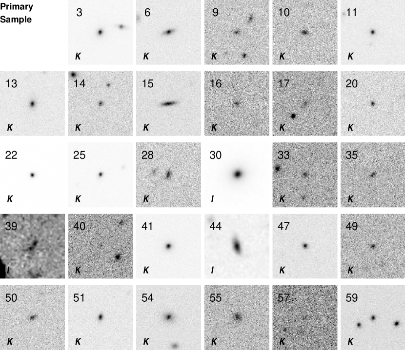
Figure 1.— Thumbnail images of the identified 6.7 $\mu$m sources. The images were taken from the data where the actual identifications were performed (IDs in TableFAINT 6.7 $\mu$m GALAXIES AND THEIR CONTRIBUTIONS TO THE STELLAR MASS DENSITY IN THE UNIVERSE). This imaging band and the name of the 6.7 $\mu$m source were overlaid on each 18 $\times$ 18 arcsec panel, an area of $3\times 3$ pixels for the ISOCAM 6 arcsec pixel-field-of-view mode. The identified sources were centered in the images. North is up and east to the left.

Fig. 1.— Continued.

Figure 2.— $f_{\nu}(6.7\,\mu\mathrm{m})/f_{\nu}(K)$ vs $B-I$ colors for the identified 6.7 $\mu$m galaxies. The sources in the primary and supplementary samples (Sect. 2) are shown with filled and empty circles, respectively. One sigma error bars are marked only for the primary sources. For sources which have enough information, their color limits are also indicated. We overlaid model predictions with the GRASIL SED library (Appendix A). Galaxies with star formation histories of the E, Sa, and Sc types (Fig. 14) are shown with dashed, dotted, and solid lines, respectively. The assumed formation redshifts are $z_{\mathrm{f}}=2$, 3, and 10 (thick, medium, and thin lines, respectively). Triangles mark positions for $z=0$, 1, 2, and 3 (for $z<z_{\rm f}$; filled triangles for $z=0$). In the upper-left region of the plot separated by the dot-dashed line, i.e., $B-I>3\log(f_{\nu}(6.7\,\mu\mathrm{m})/f_{\nu}(K)/2)+5$, we can identify a group of galaxies marked with squares (type I). They are consistent with the evolving E galaxies at $z=0$–1, or the Sa galaxies at $z=0$–1 with high formation redshifts. It should be noted that the ages of galaxies with $z_{\mathrm{f}}=2$, 3, and 10 at $z=1$ are 2.5 Gyr, 3.6 Gyr, and 5.3 Gyr, respectively, in our adopted cosmology. Thus, type I galaxies will be matured systems with old stellar populations created by vigorous star formation episodes a long time ago (see Fig. 14).

Figure 3.— $f_{\nu}(6.7\,\mu\mathrm{m})/f_{\nu}(I)$ vs $B-K$ colors for the identified 6.7 $\mu$m galaxies. Symbols are the same as in Fig. 2, although plotted sources are slightly different due to different color sets used. This diagram divides galaxies in the lower-right region of Fig. 2 into two types. All the sources above the dot-dashed line, i.e., $B-K>-1.7\log(f_{\nu}(6.7\,\mu\mathrm{m})/f_{\nu}(I))+7.3$, which have red colors both in $f_{\nu}(6.7\,\mu\mathrm{m})/f_{\nu}(I)$ and $B-K$, are marked with diamonds (type II). The GRASIL SED predictions show that type II galaxies are $z>1$ galaxies with intense star formation (evolving E or Sa galaxies). They are consistent with being ancestors of type I galaxies (squares). The remaining blue galaxies are categorized as type III. They have the colors of the evolving Sc galaxies or the E or Sa progenitors at $z\sim z_{\mathrm{f}}$, suggesting on-going star formation.

Figure 4.— Some examples of the SED fits used to derive photometric redshifts. Detections are shown with squares, in which flux errors and band widths are indicated with vertical and horizontal bars. Arrows are $3\,\sigma$ upper limits. Source names and their photometric redshifts $z_{\rm ph}$ are given with their color types, GRASIL SED names, and $\chi^{2}$ values (in parentheses).

Figure 5.— Comparison of photometric redshift estimates to spectroscopic redshift measurements. The photometric redshifts were derived as in Sect. 4.2.1 and their nominal 90 % confidence limits are shown with vertical bars. Almost all the estimates are within one sigma ranges (0.2 dex; dotted lines) from the unity relation (solid line). The primary and supplementary sample galaxies (Sect. 2) are shown with filled and empty symbols, respectively.

Figure 6.— 6.7 $\mu$m fluxes as a function of redshift. Sources with spectroscopic redshifts are indicated with double circles. For photometric redshifts, their 90 % confidence limits are indicated with horizontal bars. Vertical bars are one sigma flux errors. Galaxies in the primary sample are shown with filled circles, while the supplementary sources are marked with empty circles with no error bars. Letters, ’X’, ’S’, and ’R’ indicate the X-ray, submillimeter, and radio counterparts in Table FAINT 6.7 $\mu$m GALAXIES AND THEIR CONTRIBUTIONS TO THE STELLAR MASS DENSITY IN THE UNIVERSE, respectively. Dashed, dotted, and solid lines are model predictions for the GRASIL evolving E, Sa, and Sc galaxies, respectively (Appendix A). For each SED, formation redshifts are assumed to be $z_{\mathrm{f}}=2$, 3, and 10 (thick, medium, and thin lines, respectively).

Figure 7.— $K$ magnitudes of the 6.7 $\mu$m galaxies. Symbols are the same as in Fig. 6. Some of the 6.7 $\mu$m sources are shown with their upper or lower magnitude limits, or not shown due to the lack of their $K$ photometry (Table FAINT 6.7 $\mu$m GALAXIES AND THEIR CONTRIBUTIONS TO THE STELLAR MASS DENSITY IN THE UNIVERSE). For reference, a $K>20$ spectroscopic sample (Cowie et al., 1996) is overlaid with small squares. The 6.7 $\mu$m-selected sample does not include faint $K$ sources at low redshifts, some of which are even fainter than the GRASIL evolving Sc galaxy predictions.

Figure 8.— $I-K$ colors of the 6.7 $\mu$m galaxies. Symbols are the same as in Fig. 7. The 6.7 $\mu$m-selected sample does not include blue $I-K$ sources at low redshifts, some of which are even bluer than the GRASIL evolving Sc galaxy predictions.

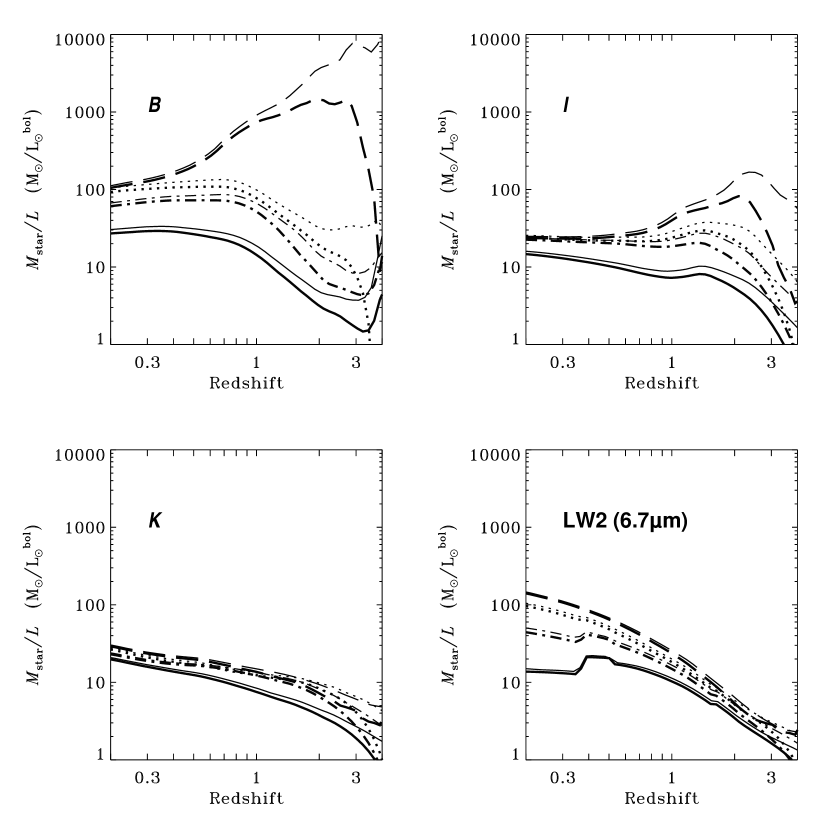
Figure 9.— Stellar mass-to-light ratios as a function of redshift. They are estimated for observations at the $B$, $I$, $K$, and ISOCAM LW2 (6.7 $\mu$m) bands. The in-band luminosity at each observing band corresponds to different wavelength with increasing redshift. Thus, for the calculation of the ratios, we adopt luminosities in units of the bolometric luminosity of the Sun (1 L${}_{\odot}^{\mathrm{bol}}=3.85\times 10^{26}$ [W]). The GRASIL models for the evolving E, Sa, Sb, and Sc galaxies are shown with dashed, dotted, dot-dashed, and solid lines, respectively. Two formation redshifts are assumed; $z_{\mathrm{f}}=5$ and 10 (thick and thin lines, respectively).

Figure 10.— Stellar masses of the 6.7 $\mu$m galaxies. Symbols are the same as in Fig. 6. The stellar masses are derived from 6.7 $\mu$m luminosities at $z>1$ or $K$ band luminosities otherwise. If no $K$ band luminosities are available, $I$ band luminosities are used instead. Note that errors in stellar mass come mainly from errors in photometry, not from errors in stellar mass-to-light ratios derived from the SED fit. A horizontal dot-dashed line indicates a characteristic stellar mass of local galaxies (Cole et al., 2001). A dashed line shows stellar mass predictions assuming the GRASIL evolving E galaxy with a formation redshift of $z_{\mathrm{f}}=10$. They are scaled to the minimum 6.7 $\mu$m flux of the primary sample (12 $\mu$Jy). This curve itself is useful to indicate the redshift dependence of the detection limit especially at the high redshift end where the scaling from the GRASIL model is almost unity. However, the scaling factor becomes very small, $\sim 0.03$ (0.1 $M_{\mathrm{star}}^{*}$) at $z=0.2$ (Appendix A). So, the uncertainties of the dashed line at the low redshift will be large. Moreover, 6.7 $\mu$m fluxes start to be affected by dust emission at such low redshifts. Note that stellar masses were derived from $K$ fluxes at $z<1$.

Figure 11.— Stellar mass functions at four epochs. For a local stellar mass function, the stepwise maximum likelihood estimates for a Salpeter IMF are reproduced from Cole et al. (2001). The accompanying errors are plotted, though almost all are within symbols for values (diamonds). This local stellar mass function is reproduced in three higher redshift panels (dashed lines). In each of these panels, our stellar mass function estimates are shown with solid and double circles for the combined (photometric and spectroscopic) and for the spectroscopic samples, respectively. Double circles are shifted slightly. Vertical errors are uncertainties in $V_{\mathrm{max}}$ and Poisson statistics. Horizontal errors are mean fractional errors in stellar mass.

Figure 12.— Redshift dependence of integrated stellar mass functions. Lower stellar mass thresholds are those in Drory et al. (2001). Our estimates are shown as in Fig. 11. Drory et al. (2001)’s values are represented as squares with vertical error bars indicating their field-to-field fluctuations. Diamonds show local values calculated from a stellar mass function by Cole et al. (2001).

Figure 13.— Stellar mass density in the universe as a function of redshift. The right axis shows densities normalized to the critical density of the universe. The contributions of the 6.7 $\mu$m galaxies are shown with solid and double circles for the combined and spectroscopic samples, respectively. The double circles are plotted at slightly lower redshifts. The horizontal bars represent the redshift ranges of the bins and the vertical bars show one sigma errors, taking account of Poisson noise and uncertainties in stellar mass and $V_{\mathrm{max}}$. Several other estimates are overlaid; solid squares are a $K$ band selected sample with photometric redshifts (Fontana et al., 2003), empty squares are an $H$ band selected sample with photometric redshifts (Dickinson et al., 2003), the diamond is a $J$ band selected spectroscopic sample (Cole et al., 2001), empty circles are an $I$ band selected spectroscopic sample (Brinchmann & Ellis, 2000), X marks are an $R$ band selected spectroscopic sample (Cohen, 2002), and triangles are an $R^{\prime}$ band selected photometric sample around a $z=4.7$ quasar (Giallongo et al., 1998). The empty/solid squares and the diamond are obtained from full integration of a Schechter fit to their respective luminosity or stellar mass function at each redshift bin. The X marks and the empty circles are quasi-fully integrated values with a finite integration range from 10 $L^{*}$ to 1/20 $L^{*}$, and $10.5<\log(M_{\mathrm{star}}[h_{65}^{-2}$ M${}_{\odot}])<11.6$, respectively. The triangles are simply summed values of the detected sources like ours. We adopted her mean redshifts for Cohen (2002) and all four cases discussed in Dickinson et al. (2003) for their error bars. Miller-Scalo IMFs were used in Giallongo et al. (1998). All points plotted here were normalized to our cosmology and a Salpeter IMF with mass limits of 0.1 M_⊙ and 125 M_⊙. The two dashed curves are deduced by integrating the star formation rate density in the universe, which is derived from the UV luminosity density as a function of redshift (Cole et al., 2001). The upper curve is an extinction corrected case for $E(B-V)=0.15$, and the lower one has no dust correction.

Figure 14.— Star formation rates (SFRs) for the evolving E, Sa, Sb, and Sc galaxies in the GRASIL library (Appendix A). They are shown as a function of age with dashed, dotted, dot-dashed, and solid lines, respectively. It should be noted that age increases from left to right. After the age of 1 Gyr, the E galaxy was assumed to stop its star formation because of a galactic wind.

Table 1 Source Identifications in the Optical and Near-Infrared

Name	R.A.	Decl.	$r_{0}$	6.7 $\mu$m	S/N	ID	$r_{1}$	$P_{\mathrm{t}}$	$P_{\mathrm{c}}$	$P_{\mathrm{t}}/P_{\mathrm{c}}$	$P_{\mathrm{t}}/P_{\mathrm{c}}^{(2)}$
#	(J2000.0)		(″)	($\mu$Jy)			(″)
Primary Sample
3	13 12 18.09	+42 43 45.0	1.1	$50$	$11.4$	$K$	0.8	0.49	0.000056	string880.
6	13 12 18.32	+42 43 19.2	1.1	$66$	$11.9$	$K$	0.5	0.63	0.000038	string1700.
9	13 12 19.48	+42 45 36.4	1.5	$25$	$5.8$	$K$	0.5	0.75	0.00069	string110.
10	13 12 20.01	+42 44 38.4	1.4	$21$	$6.4$	$K$	0.7	0.64	0.0015	string41.
11	13 12 21.02	+42 44 33.8	1.5	$19$	$5.9$	$K$	1.0	0.49	0.00094	string53.	string3.7
13	13 12 21.39	+42 44 23.4	1.4	$24$	$7.0$	$K$	0.3	0.80	0.000092	string870.
14	13 12 21.57	+42 44 05.8	1.5	$19$	$6.3$	$K$	0.8	0.58	0.0023	string25.
15	13 12 21.58	+42 45 18.8	1.0	$60$	$15.6$	$K$	0.3	0.77	0.000086	string900.
16	13 12 21.89	+42 43 45.5	1.5	$19$	$5.8$	$K$	2.3	0.12	0.031	string3.8
17	13 12 22.53	+42 44 50.9	1.5	$17$	$5.3$	$K$	0.3	0.86	0.00053	string160.	string0.14
20	13 12 23.65	+42 45 16.9	1.5	$20$	$6.2$	$K$	2.9	0.048	0.032	string1.5
22	13 12 23.91	+42 45 43.5	0.9	$135$	$28.5$	$K$	1.1	0.25	0.0000023	11000.
25	13 12 24.90	+42 44 14.8	1.1	$39$	$11.7$	$K$	2.5	0.023	0.0014	string16.
27	13 12 25.2string	+42 46 00string	1.2	$45$	$10.1$
28	13 12 25.18	+42 43 44.9	1.3	$27$	$7.9$	$K$	1.3	0.34	0.0042	string82.	string2.8
30	13 12 26.31	+42 42 26.9	1.6	$70$	$5.0$	$I$	0.9	0.59	0.000025	string2300.
33	13 12 27.32	+42 44 49.7	1.5	$17$	$5.4$	$K$	1.4	0.36	0.0087	string41.	string0.032
35	13 12 27.70	+42 45 36.6	1.7	$15$	$4.8$	$K$	1.3	0.44	0.0059	string75.
39	13 12 28.44	+42 46 03.3	1.5	$27$	$5.4$	$I$	1.4	0.35	0.0078	string45.
40	13 12 28.29	+42 44 54.6	1.7	$14$	$4.8$	$K$	3.4	0.047	0.084	string0.56
41	13 12 28.58	+42 43 58.9	1.1	$46$	$13.3$	$K$	1.0	0.37	0.00016	string240.
44	13 12 29.21	+42 45 58.2	1.3	$37$	$8.2$	$I$	1.1	0.42	0.00032	string130.
47	13 12 29.88	+42 44 08.5	1.5	$16$	$5.3$	$K$	0.7	0.64	0.00049	string130.	string0.19
49	13 12 30.10	+42 44 20.7	1.6	$15$	$5.0$	$K$	1.3	0.42	0.0071	string60.	string0.14
50	13 12 30.16	+42 44 56.5	1.5	$19$	$5.8$	$K$	2.4	0.11	0.015	string7.3	string0.11
51	13 12 31.05	+42 43 32.6	1.4	$22$	$6.7$	$K$	0.6	0.66	0.00025	string260.
54	13 12 31.50	+42 45 52.2	0.9	$167$	$23.6$	$K$	1.2	0.20	0.000095	string210.
55	13 12 31.90	+42 43 46.4	1.9	$12$	$4.3$	$K$	2.1	0.25	0.010	string25.
57	13 12 31.94	+42 44 29.7	1.5	$18$	$6.2$	$K$	2.2	0.13	0.033	string3.9
59	13 12 33.92	+42 44 42.7	1.6	$18$	$5.0$	$K$	1.2	0.47	0.00099	string47.	20.
61	13 12 34.68	+42 43 42.8	1.3	$55$	$8.3$	$K$	2.5	0.058	0.0024	string24.
62	13 12 34.51	+42 43 09.3	1.8	$88$	$4.5$	$I$	2.1	0.25	0.00056	string45.
64	13 12 35.90	+42 43 58.0	1.3	$107$	$7.7$	$B$	2.0	0.14	0.000074	string190.
Supplementary Sample
0	13 12 15.79	+42 44 00.3	2.5	$19$	$2.7$	$K$	0.6	0.80	0.00013	string600.
1	13 12 16.8string	+42 44 21string	1.9	$18$	$4.1$
2	13 12 17.10	+42 44 52.2	2.3	$14$	$3.0$	$I_{814}$	3.1	0.18	0.11	string1.6	string0.17
4	13 12 17.82	+42 45 27.3	2.3	$18$	$3.2$	$K$	2.6	0.25	0.044	string5.6
5	13 12 18.1string	+42 46 15string	2.6	$34$	$2.7$
7	13 12 18.7string	+42 42 48string	2.3	$66$	$3.0$
8	13 12 19.34	+42 45 01.1	1.9	$12$	$4.0$	$K$	2.0	0.29	0.0065	string44.
12	13 12 21.19	+42 46 26.0	2.3	$63$	$3.0$	$I$	2.0	0.39	0.015	string26.	string4.0
18	13 12 22.45	+42 43 15.6	2.7	$8$	$2.6$	$K$	4.1	0.14	0.062	string2.2
19	13 12 23.10	+42 46 05.4	2.2	$17$	$3.3$	$K$	1.9	0.39	0.0067	string58.
21	13 12 23.30	+42 44 29.4	2.3	$9$	$3.0$	$I_{814}$	2.3	0.31	0.081	string3.9	string2.1
23	13 12 24.18	+42 43 57.7	2.3	$9$	$3.1$	$K$	2.0	0.39	0.022	string18.
24	13 12 24.33	+42 43 23.9	2.0	$12$	$3.8$	$I_{814}$	2.0	0.31	0.078	string3.9	string0.067
26	13 12 24.60	+42 45 11.4	2.1	$10$	$3.5$	$K$	2.2	0.29	0.023	string13.
29	13 12 25.56	+42 43 20.5	2.4	$8$	$2.8$	$I$	2.4	0.33	0.016	string20.	string8.5
31	13 12 26.58	+42 45 30.0	3.2	$6$	$2.4$	$I_{814}$	5.2	0.11	0.086	string1.2	string0.43
32	13 12 26.31	+42 44 04.8	2.1	$9$	$3.4$	$K$	1.3	0.55	0.011	string48.	string1.5
34	13 12 27.51	+42 46 30.4	2.4	$45$	$2.9$	$I$	2.0	0.40	0.017	string23.	string4.1
36	13 12 27.80	+42 45 09.6	2.4	$8$	$2.8$	$K$	1.0	0.66	0.0053	string13.	string0.24
37	13 12 27.9string	+42 42 20string	2.4	$87$	$2.9$
38	13 12 28.50	+42 44 28.9	2.1	$10$	$3.6$	$K$	2.6	0.23	0.0078	string29.	string7.0
42	13 12 28.9string	+42 46 19string	2.3	$32$	$3.1$
43	13 12 28.87	+42 43 04.8	2.1	$12$	$3.7$	$I$	2.5	0.23	0.021	string11.	string0.070
45	13 12 29.20	+42 44 38.7	3.0	$7$	$2.5$	$K$	2.5	0.39	0.020	string20.	string3.5
46	13 12 29.69	+42 43 00.1	2.3	$11$	$3.2$	$I$	1.1	0.63	0.0072	string88.	string2.0
48	13 12 29.9string	+42 45 14string	2.3	$9$	$3.1$
52	13 12 31.76	+42 42 42.7	2.3	$24$	$3.2$	$I$	3.4	0.14	0.066	string2.2	string0.34
53	13 12 31.5string	+42 42 36string	2.9	$27$	$2.5$
56	13 12 31.86	+42 45 04.1	2.4	$8$	$2.9$	$K$	1.4	0.55	0.0080	string68.
58	13 12 32.78	+42 43 12.4	2.6	$15$	$2.7$	$I$	1.6	0.53	0.018	string29.	16.
60	13 12 34.31	+42 46 00.3	3.3	$26$	$2.3$	$I$	2.4	0.47	0.012	string38.	string5.9
63	13 12 34.81	+42 45 05.1	2.1	$18$	$3.7$	$K$	2.6	0.21	0.017	string12.
Negative Sample
Nstring0	13 12 17.9string	+42 45 11string	2.2	$-17$	$-3.3$
Nstring1	13 12 19.5string	+42 45 47string	2.2	$-13$	$-3.4$
Nstring2	13 12 20.0string	+42 43 33string	3.3	$-6$	$-2.3$
Nstring3	13 12 23.6string	+42 45 28string	2.1	$-10$	$-3.4$
Nstring4	13 12 24.8string	+42 44 37string	2.6	$-7$	$-2.6$
Nstring5	13 12 25.5string	+42 42 04string	2.2	$-125$	$-3.3$
Nstring6	13 12 30.5string	+42 45 37string	1.9	$-11$	$-4.0$
Nstring7	13 12 31.46	+42 44 26.0	2.0	$-11$	$-3.8$	$I_{814}$	2.9	0.15	0.085	string1.7	string1.3
Nstring8	13 12 32.9string	+42 45 13string	2.3	$-9$	$-3.2$
Nstring9	13 12 34.23	+42 43 27.3	3.3	$-17$	$-2.3$	$I$	2.3	0.49	0.037	string13.	string1.7
N10	13 12 35.76	+42 44 43.7	2.0	$-26$	$-3.9$	$I$	4.2	0.032	0.0067	string4.7	string0.15
N11	13 12 38.7string	+42 44 38string	3.3	$-69$	$-2.3$

Note. — Source identification results with the probability ratio method described in Sect. 3.1. The contents are divided into three sub samples; the primary, supplementary, and negative samples (Sect. 2). Names, coordinates, their one sigma errors ($r_{0}$), and total 6.7 $\mu$m fluxes are extracted from Sato et al. (2003). The coordinates of the successfully identified sources are updated with their optical or near-infrared positions in the identifying image, which is indicated in the ID column. Listed signal-to-noise ratios (S/Ns) are derived from standard deviations of the co-added images at the source position using a 7.2 arcsec aperture. Thus both photon noise and undersampling effects are included. With raster observations, pixel values could range from $\sim 25$ % to $\sim 100$ % of source fluxes depending on exact locations of the sources on the ISOCAM 6 arcsec pixels, giving high standard deviations at source positions. At 6.7 $\mu$m, an Airy disk size is 5.6 arcsec for the ISO telescope. Note that errors in total 6.7 $\mu$m fluxes are much larger than that can be inferred from these detection S/N values. Derivation of total fluxes and their associated errors are described in Sato et al. (2003). For each identification, we list the distance between the 6.7 $\mu$m source and the identified source in the ID image ($r_{1}$). Two probabilities that the identified source is a true association ($P_{\mathrm{t}}$) or a chance association ($P_{\mathrm{c}}$), and their ratio are also shown. The last column shows the second highest probability ratio for sources within a distance of 3 $r_{0}$ from the original 6.7 $\mu$m position. The contents for the negative sample are the same but with negative flux and S/N values.

Table 2 Source Identifications at the X-ray, Submillimeter, and Radio Wavelengths

Note. — Source identifications of the mid-infrared (ISOCAM/LW2) sources in the SSA13 field with X-ray (Chandra), submillimeter (JCMT/SCUBA), and radio (VLA/FIRST) sources (Mushotzky et al., 2000; Barger et al., 2001, 1998, 1999; White et al., 1997). No data are indicated with ’ $\cdots$ ’. Flux limits are no detections at a level of 3 $\sigma$. Listed offsets $d_{\mathrm{X}}$, $d_{\mathrm{S}}$, and $d_{\mathrm{R}}$ are measured from the optical or near-infrared positions of the 6.7 $\mu$m sources in Table FAINT 6.7 $\mu$m GALAXIES AND THEIR CONTRIBUTIONS TO THE STELLAR MASS DENSITY IN THE UNIVERSE.

Table 3 Properties of the Mid-Infrared Sources

Note. — Properties of the primary and supplementary 6.7 $\mu$m samples. Magnitudes at the $K$, $I$, and $B$ bands are corrected total magnitudes as in Cowie et al. (1996). Measurements with a 3″ aperture are corrected with an average offset. No data are indicated with ’ $\cdots$ ’. Upper flux limits are no detections at a level of 3 $\sigma$. Lower flux limits are real measurements for saturated sources or for sources at the image boundaries. Except two stars, the remaining sources are divided into three color types (Sect. 4.1) using the GRASIL SED library (Appendix A). Spectroscopic redshifts $z_{\mathrm{sp}}$ (Songaila et al., 1994; Cowie et al., 1996; Barger et al., 2001) are listed with no error information, while photometric redshifts $z_{\mathrm{ph}}$ are shown with their 90 % confidence limits. Photometric redshifts $z_{\mathrm{ph}}$ are derived with fits to the GRASIL evolving templates and local ones (Sect. 4.2.1), while stellar masses $M_{\mathrm{star}}$ are derived with fits to the GRASIL evolving templates only (Sect. 5.2). The results of these two fits are shown separately as (SED₁, $\chi^{2}_{1}$) and (SED₂, $\chi^{2}_{2}$). The name of best-fit SED is listed with its age in Gyr for the case of the evolving SED. The local template for giant ellipticals is marked as GE. Just after the $\chi^{2}$ value, ancillary information on the fit are shown in parenthesis. For example, d3/4 means that 3 detections among 4 photometric data were used to determine the best-fit and the resulting $\chi^{2}$ value. The remaining one flux limit was checked its consistency to the fit. In case of u1/4, one upper flux limit (non-detection) found to be inconsistent with the initial best-fit derived with the remaining three detections. Then, the normalization of the initial fit was decreased down to the upper limit and the $\chi^{2}$ value was evaluated with this re-normalized spectrum.

Table 4 Stellar Mass Functions and Stellar Mass Densities

$z$ Range	$\log\Phi(M_{\mathrm{star}},z)$				$\log\rho_{\mathrm{star}}(z)$
	$(h_{65}^{3}\,\mathrm{Mpc}^{-3}\,\mathrm{dex}^{-1})$				($h_{65}$ M⊙ Mpc-3)
	$\log M_{\mathrm{star}}$ range
	($h_{65}^{-2}$ M⊙)
	10.15 – 10.55	10.55 – 10.95	10.95 – 11.35	11.35 – 11.75
Combined Sample
0.2–0.5	$-2.3^{+0.5}_{-0.5}$ (3)	$-2.2^{+0.3}_{-0.4}$ (4)	$-2.3^{+0.3}_{-0.3}$ (5)	$\cdots$	$8.7^{+0.2}_{-0.2}$ (12)
0.5–1.2	$\cdots$	$-2.5^{+0.5}_{-0.6}$ (4)	$-2.9^{+0.3}_{-0.3}$ (6)	$-3.8^{+0.7}_{-1.0}$ (1)	$8.2^{+0.3}_{-0.3}$ (11)
1.2–3.0	$\cdots$	$\cdots$	$-3.3^{+0.4}_{-0.5}$ (5)	$-4.0^{+0.5}_{-0.7}$ (2)	$7.6^{+0.3}_{-0.4}$ ( 7)
Spectroscopic Sample
0.2–0.5	$-2.5^{+0.4}_{-0.6}$ (2)	$-2.4^{+0.3}_{-0.5}$ (3)	$-2.3^{+0.3}_{-0.3}$ (5)	$\cdots$	$8.6^{+0.2}_{-0.3}$ (10)
0.5–1.2	$\cdots$	$-2.5^{+0.5}_{-0.6}$ (4)	$-3.2^{+0.4}_{-0.5}$ (3)	$\cdots$	$8.1^{+0.4}_{-0.4}$ ( 7)
1.2–3.0	$\cdots$	$\cdots$	$-3.7^{+0.9}_{-1.4}$ (1)	$\cdots$	$6.9^{+0.9}_{-1.5}$ ( 1)

Note. — Epoch dependent stellar mass functions $\Phi(M_{\mathrm{star}},z)$ and stellar mass densities $\rho_{\mathrm{star}}(z)$. They are derived from the 6.7 $\mu$m primary sample. Two sets of estimates are obtained; one with the combined (photometric and spectroscopic) sample and the other with the spectroscopic sample. One sigma errors are estimated from uncertainties in $V_{\mathrm{max}}$ and Poisson statistics. For stellar mass densities, errors in stellar mass are also taken into account. Numbers in parentheses are the numbers of 6.7 $\mu$m galaxies used in the calculation.

References

- Altieri et al. (1999) Altieri, B., et al. 1999, A&A, 343, L65
- Aussel et al. (1999) Aussel, H., Cesarsky, C. J., Elbaz, D., & Starck, J. L. 1999, A&A, 342, 313
- Avni (1976) Avni, Y. 1976, ApJ, 210, 642
- Barger et al. (1998) Barger, A. J., Cowie, L. L., Sanders, D. B., Fulton, E., Taniguchi, Y., Sato, Y., Kawara, K., & Okuda, H. 1998, Nature, 394, 248
- Barger et al. (1999) Barger, A. J., Cowie, L. L., & Sanders, D. B. 1999, ApJ, 518, L5
- Barger et al. (2001) Barger, A. J., Cowie, L. L. Mushotzky, R. F., & Richards, E. A. 2001, AJ, 121, 662
- Bolzonella, Miralles, & Pelló (2000) Bolzonella, M., Miralles, J.-M., & Pelló, R. 2000, A&A, 363, 476
- Brinchmann & Ellis (2000) Brinchmann, J. & Ellis, R. S. 2000, ApJ, 536, L77
- Carilli & Yun (2000) Carilli, C. L. & Yun, M. S. 2000, ApJ, 530, 618
- Carroll, Press, & Turner (1992) Carroll, S. M., Press, W. H., & Turner, E. L. 1992, ARA&A, 30, 499
- Cesarsky et al. (1996) Cesarsky, C. J., et al. 1996, A&A, 315, L32
- Cohen (2002) Cohen, J. G. 2002, ApJ, 567, 672
- Cole et al. (2001) Cole, S., et al. 2001, MNRAS, 326, 255
- Condon et al. (1998) Condon, J. J., Cotton, W. D., Greisen, E. W., Yin, Q. F., Perley, R. A., Taylor, G. B., & Broderick, J. J. 1998, AJ, 115, 1693
- Cowie et al. (1994) Cowie, L. L., Gardner, J. P, Hu, E. M., Songaila, A., Hodapp, K.-W., & Wainscoat, R. J. 1994, ApJ, 434, 114
- Cowie, Hu, & Songaila (1995) Cowie, L. L., Hu, E. M., & Songaila, A. 1995, AJ, 110, 1576
- Cowie et al. (1996) Cowie, L. L., Songaila, A., Hu, E. M., & Cohen, J. G. 1996, AJ, 112, 839
- Dickinson et al. (2003) Dickinson, M., Papovich, C., Ferguson, H. C., & Budavári, T. 2003, ApJ, 587, 25
- Drory et al. (2001) Drory, N., Bender, R., Snigula, J., Feulner, G., Hopp, U., Maraston, C., Hill, G. J., & de Oliveira, C. M. 2001, ApJ, 562, L111
- Elbaz et al. (1999) Elbaz, D., et al. 1999, A&A, 351, L37
- Flores et al. (1999a) Flores, H., et al. 1999a, A&A, 343, 389
- Flores et al. (1999b) Flores, H., et al. 1999b, ApJ, 517, 148
- Fontana et al. (2003) Fontana, A. J., et al. 2003, ApJ, 594, L9
- Franceschini et al. (2001) Franceschini, A., Aussel, H., Cesarsky, C. J., Elbaz, D., & Fadda, D. 2001, A&A, 378, 1
- Franceschini et al. (2003) Franceschini, A., et al. 2003, A&A, 403, 501
- Genzel & Cesarsky (2000) Genzel, R. & Cesarsky, C. J. 2000, ARA&A, 38, 761
- Giallongo et al. (1998) Giallongo, E., D’Odorico, S., Fontana, A., Cristiani, S., Egami, E., Hu, E., & McMahon, R. G. 1998, AJ, 115, 2169
- Hasinger (2000) Hasinger, G. 2000, in Lecture Notes in Physics, 548, ISO Survey of a Dusty Universe, ed. D. Lemke, M. Stickel, and K. Wilke, 423
- Hogg et al. (1998) Hogg, D. W., et al. 1998, AJ, 115, 1418
- Hogg (1999) Hogg, D. W. 1999, astro-ph/9905116
- Hughes et al. (1998) Hughes, D. H., et al. 1998, Nature, 394, 241
- Iwasawa (1999) Iwasawa, K. 1999, MNRAS, 302, 96
- Kessler et al. (1996) Kessler, M. F., et al. 1996, A&A, 315, L27
- Maihara et al. (2001) Maihara, T., et al. 2001, PASJ, 53, 25
- Mann et al. (1997) Mann, R. G., et al. 1997, MNRAS, 289, 482
- Metcalfe et al. (2003) Metcalfe, L., et al. 2003, A&A, 407, 791
- Metcalfe et al. (2001) Metcalfe, N., Shanks, T., Campos, A., McCracken, H. J., & Fong, R. 2001, MNRAS, 323, 795
- Mushotzky et al. (2000) Mushotzky, R. F., Cowie, L. L., Barger, A. J., & Arnaud, K. A. 2000, Nature, 404, 459
- Oliver et al. (2002) Oliver, S., et al. 2002, MNRAS, 332, 536
- Salpeter (1955) Salpeter, E. E. 1955, ApJ, 121, 161
- Sato et al. (2002) Sato, Y., Cowie, L. L., Kawara, K., Taniguchi, Y., Sofue, Y., Matsuhara, H., & Okuda, H. 2002, ApJ, 578, L23
- Sato et al. (2003) Sato, Y., et al. 2003, A&A, 405, 833
- Sawicki (2002) Sawicki, M. 2002, AJ, 124, 3050
- Serjeant et al. (1997) Serjeant, S. B. G., et al. 1997, MNRAS, 289, 457
- Silva et al. (1998) Silva, L., Granato, G. L., Bressan, A., & Danese, L. 1998, ApJ, 509, 103, http://web.pd.astro.it/granato/grasil/grasil.html
- Solanes, Salvador-Sole, & Sanroma (1989) Solanes, J. M., Salvador-Sole, E., & Sanroma, M. 1989, AJ, 98, 798
- Songaila et al. (1994) Songaila, A., Cowie, L. L., Hu, E. M., & Gardner, J. P. 1994, ApJS, 94, 461
- Steidel et al. (1999) Steidel, C. C., Adelberger, K. L., Giavalisco, M., Dickinson, M., & Pettini, M. 1999, ApJ, 519, 1
- Takeuchi et al. (2000) Takeuchi, T. T., Yoshikawa, K., & Ishii, T. T. 2000, ApJS, 129, 1
- Taniguchi et al. (1997) Taniguchi, Y., et al. 1997, A&A, 328, L9
- White et al. (1997) White, R. L., Becker, R. H., Helfand, D. J., & Gregg, M. D. 1997, ApJ, 475, 479