The Star Formation History of the Small Magellanic Cloud

Abstract

We present the spatially-resolved star formation and chemical enrichment history of the Small Magellanic Cloud (SMC) across the entire central $4^{\circ}\times 4.5^{\circ}$ area of the main body, based on $UBVI$ photometry from our Magellanic Clouds Photometric Survey. We find that 1) approximately 50% of the stars that ever formed in the SMC formed prior to 8.4 Gyr ago ($z>1.2$ for WMAP cosmology), 2) the SMC formed relatively few stars between 8.4 and 3 Gyr ago, 3) there was a rise in the mean star formation rate during the most recent 3 Gyr punctuated by “bursts” at ages of 2.5, 0.4, and 0.06 Gyr, 4) the bursts at 2.5 and 0.4 Gyr are temporally coincident with past perigalactic passages of the SMC with the Milky Way, 5) there is preliminary evidence for a large-scale annular structure in the 2.5 Gyr burst, and 6) the chemical enrichment history derived from our analysis is in agreement with the age-metallicity relation of the SMC’s star clusters. Consistent interpretation of the data required an ad hoc correction of 0.1–0.2 mag to the B-V colors of 25% of the stars; the cause of this anomaly is unknown, but we show that it does not strongly influence our results.

1 Introduction

Determinations of detailed, quantitative star formation histories (SFHs) of local galaxies aim to provide an empirical foundation upon which a comprehensive theory of star formation in galaxies can be constructed. Presently, even basic questions of how star formation proceeds on galactic scales remain unanswered. Do galaxies form stars continuously, or in bursts separated by epochs of relative quiescence? If star formation occurs in bursts, what processes mediate the bursts? Major galaxy interactions are known to induce vigorous star-formation events (e.g.,  Larson & Tinsley, 1978; Lonsdale et al., 1984; Cutri & McAlary, 1985), but do less-dramatic interaction events also trigger significant star formation? Are parametrizations describing stellar populations, such as the initial mass function (IMF) or the cluster-to-field star ratio, determined by the integrated dynamical interaction history of a galaxy, or are they universal? How significant are gas inflow and outflow to the chemical enrichment history of galaxies?

These long-standing questions can be addressed directly by studying the detailed SFHs of Local Group galaxies. The Magellanic Clouds are optimal targets for SFH analysis because 1) their proximity allows us to obtain color-magnitude diagrams (CMDs) of resolved stellar populations well down the main sequence and measure a bulk proper motion from which their space velocity and orbit can be derived, 2) their proximity to the Milky Way (and to each other) suggests that tidal interactions may play an important, periodic role in triggering star formation, and 3) their on-going star formation enables us to measure star formation events at recent times, where we can achieve the high temporal resolution necessary to investigate possible triggering mechanisms and the the high spatial resolution necessary to investigate the interplay between star formation and the interstellar medium.

Previous studies of the Clouds have resulted in tantalizing glimpses of their SFHs. For example, the “age-gap” among LMC clusters (van den Bergh, 1991; Da Costa, 1991; Girardi et al., 1995; Westerlund, 1997) suggests that there was a long period of quiescence in its history. In a photographic-plate study of the outer regions of the SMC, Gardiner & Hatzidimitriou (1992) found that the bulk of the stellar population is about 10 Gyr old, with about 7% of the population aged 15–16 Gyr, and also observed a young stellar population biased toward the eastern, LMC-facing side of the SMC. Crowl et al. (2001) see a similar trend among the SMC’s populous clusters: those on the eastern side tend to be younger and more metal-rich than those on the western side. Finally, several authors have performed SFH analyses on HST/WFPC2 fields in both Clouds, offering detailed snapshots of the histories of specific regions in these galaxies (Gallagher et al., 1996; Ardeberg et al., 1997; Holtzman et al., 1999; Olsen, 1999; Dolphin et al., 2001; Smecker-Hane et al., 2002). However, there has not yet been an attempt to determine the full, global star-formation history of either Magellanic Cloud, because a sufficiently sensitive, spatially comprehensive catalog of their stellar populations had not been available prior to our Magellanic Clouds Photometric Survey (MCPS; Zaritsky et al. (1997)).

In this article, we present the global star-formation history of the Small Magellanic Cloud, based on the MCPS $UBVI$ catalog that includes over six million SMC stars. We briefly review the MCPS and the StarFISH star-formation history reconstruction program Harris & Zaritsky (2001) in Section 2.1. The determination of the necessary inputs to StarFISH (including detailed treatments of the interstellar extinction and photometric errors) is presented in Section 2.2. We describe the application of StarFISH to the SMC catalog in Section 2.3, and our comprehensive map of the SMC’s SFH is presented in Section 2.4. Analysis and discussion of the SFH map, which shows significant structure in both the spatial and temporal dimensions, is presented in Section 3, and we summarize our findings in Section 4.

2 Deriving the SMC’s Star Formation History

2.1 A Brief Summary of the Previously Published Data and Methodology

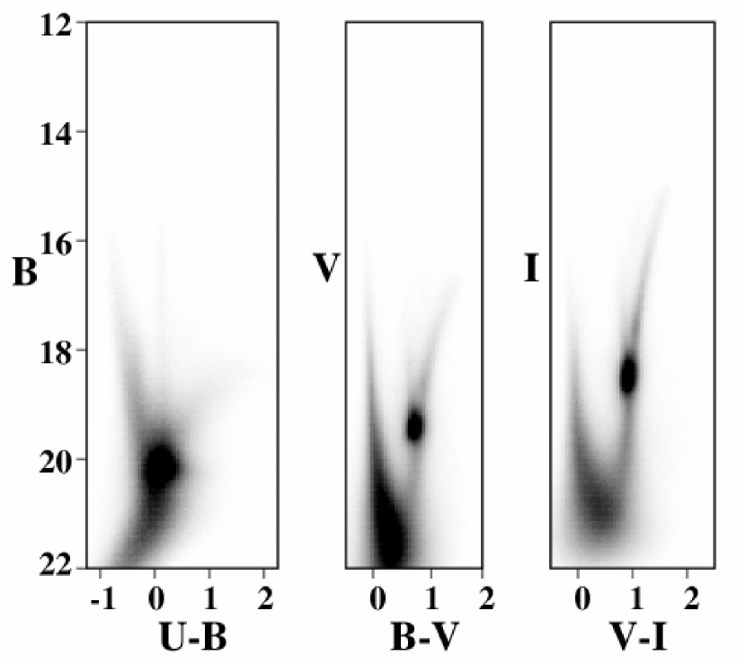
Figure 1: A “CMD triptych” illustrating our $UBVI$ photometry of six million SMC stars. Each CMD panel is a pixelized Hess diagram showing the number of stars in each pixel. The mixed populations evident in these CMDs represent a “fossil record” of a complex star-formation history in this galaxy.

Our Magellanic Clouds Photometric Survey (MCPS,  Zaritsky et al., 1997) provides the most complete optical survey of bright stellar populations in the Magellanic Clouds to date. The Survey was conducted between 1996 November and 1999 December at the Las Campanas Observatory 1-meter Swope Telescope. We employed a unique drift-scan CCD instrument (the Great Circle Camera, Zaritsky et al., 1996) which allowed us to efficiently acquire large, distortion-free scans at the extreme declinations of the Magellanic Clouds. Typical survey scans are 24$\arcmin$ wide and 2$\arcdeg$ long. Twenty-six scans cover the $4\arcdeg\times 4.5\arcdeg$ area surveyed in the SMC. Each scan was observed using $U$, $B$, $V$, and $I$ filters and the effective exposure times are $\sim$5 minutes. We use an automated data-reduction pipeline that consists of IRAF (Tody, 1986) scripts and the DAOPHOT photometry package (Stetson, 1987). The final SMC catalog (Zaritsky et al., 2002) is 50% complete to $m_{v}=21--22$ mag, depending on the local crowding conditions. The catalog includes at least $B$ and $V$ photometry for over 6 million SMC stars (see Figure 1). In the present analysis, we use a subset of the photometry with $V\leq 21$, where the completeness corrections are modest (50%–95% depending on local crowding conditions).

We developed the StarFISH package (Harris & Zaritsky, 2001) to determine the detailed star-formation histories encoded in the stellar populations of our SMC and LMC catalogs (however, the package is designed to be generally applicable to any photometric data and is available for public use). StarFISH performs a chi-squared minimization between the observed photometry and model photometry based on theoretical isochrones (we employ the Padua isochrones most recently published by Girardi et al. (2002), but the package is sufficiently flexible to use of any set of isochrones). We construct a library consisting of sets of three synthetic Hess diagrams, which we shall refer to as CMD triptychs. Each CMD triptych represents the predicted $UBVI$ photometry for a single stellar population of a specific age and metallicity. Constructing the synthetic CMD triptychs requires us to specify the distance, initial mass function, binary fraction, and the empirical models of the interstellar extinction and photometric errors. Once we have the library of synthetic CMD triptychs, we construct a composite model CMD triptych that represents the predicted photometry for any arbitrary SFH. The composite model is a linear combination of the set of synthetic CMD triptychs, each of which is modulated by an amplitude value that is equal to the number of stars present at the age and metallicity of the corresponding synthetic population. We employ an efficient downhill simplex algorithm to select the model triptych that is most similar to that observed and evaluate uncertainties by examining the parameter space about the best fit set of amplitudes (see Harris & Zaritsky, 2001). Although the fitting could be done purely in the multidimensional color space, the use of the triptych is adopted for visualizing the fits and potential systematic errors.

2.2 Defining the Inputs to StarFISH

As described broadly above, a number of parameter values must be set before running StarFISH. We adopt a distance modulus for the SMC of 18.9 mag (Dolphin et al., 2001), corresponding to $\sim 60$ kpc. For the IMF, we adopt a simple power-law with a Salpeter slope (Sirianni et al., 2002). Having little solid information to guide us in adopting a binary fraction, we simply adopt a fraction of 0.5, with secondary masses drawn randomly from the IMF (consistent with the findings of Duquennoy & Mayor, 1991). Our detailed, statistical modeling of interstellar extinction and photometric errors are discussed below.

2.2.1 The Isochrone Set

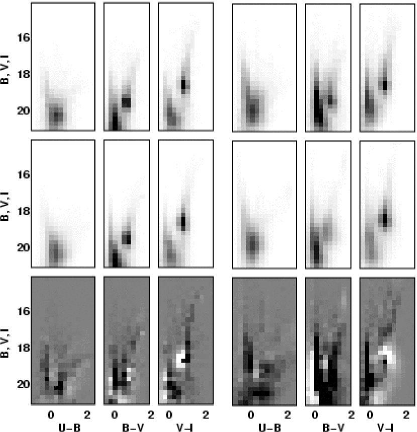
Figure 5: CMD triptychs from two regions in the SMC. At left, we show CMDs for the region labeled MK in Figure 3 (the same region as in Figure 4), which was well-fit by the StarFISH algorithm, with a reduced $\chi^{2}$ value of 3. At right, we show CMDs for region KK, which was initially poorly-fit by StarFISH, with a reduced $\chi^{2}$ value of 11.5. In each case, the top triptych shows the data photometry, the middle row shows the best-fit model photometry, and the bottom row shows the data-model difference (with black indicating an excess of data stars, and white indicating an excess of model stars). The $B-V$ difference CMD for region KK illustrates the need for a $B-V$ offset, as discussed in Section 2.3.4. After applying the $B-V$ offset, the reduced $\chi^{2}$ value for region KK drops to 2.7.

For the present analysis, we begin with a subset of the Padua isochrones (Girardi et al., 2002) for three metallicities appropriate for stellar populations in the SMC: Z=0.001, 0.004, and 0.008 (corresponding to [Fe/H]=-1.3, -0.7, and -0.4). We note that this may be a bit more metal-rich than the most metal-poor populations in the SMC. Notably, NGC 121 (the SMC’s oldest populous cluster) has [Fe/H] between -1.7 and -1.0 (Suntzeff et al., 1986; Mighell et al., 1998; Da Costa & Hatzidimitriou, 1998; de Freitas Pacheco et al., 1998; Dolphin et al., 2001). The chemical enrichment model for the SMC by Pagel & Tautvaisienė (1999) indicates rapid metal enrichment in its early history, rising above [Fe/H]=-1.3 around 11 Gyr ago (see their Figure 5). We therefore believe that the omission of more metal-poor isochrones in our analysis will not significantly impact our results, since any stellar populations with metallicity below Z=0.001 are expected only in our very oldest age bin.

We deemed it unecessary to interpolate between these three metallicity bins. Our tests show that StarFISH can account for intermediate metallicities by simply mixing amplitudes of the bounding isochrones (see analysis of NGC 1978 in Harris & Zaritsky, 2001); in other words, there are no significant “gaps” between isochrones of the same age and adjacent metallicities in our synthetic CMD triptychs. This conclusion is data-dependent, of course; higher-precision photometry than the MCPS may well require finer metallicity resolution than we use here.

For each metallicity, the Padua group provides isochrones for 62 ages distributed uniformly in log(age) between 4 Myr and 18 Gyr. This time resolution is much too fine for our purposes; when interstellar extinction and photometric errors are included, some isochrones with adjacent ages are completely degenerate. As outlined in Harris & Zaritsky (2001), we circumvent this degeneracy by “locking” together isochrones into groups of four, yielding an effective age resolution of $log(\Delta age)=0.2$. Thus, each of our synthetic CMD triptychs actually spans a range of ages, and the age bins are wide enough that no CMD triptych is completely degenerate with any other. Again, this age resolution was adopted empirically, taking the photometric error characteristics of the data into account. Our adopted synthetic CMD library consists of 47 isochrone groups; 11 ages spanning 100 Myr to 12 Gyr for Z=0.001, and 18 ages spanning 4 Myr to 12 Gyr for both Z=0.004 and Z=0.008.

2.2.2 Interstellar Extinction

In a previous analysis of the interstellar extinction in the SMC (Zaritsky, 1999), we found (a) the distribution of extinction values is much wider than can be explained by photometric errors; i.e., there is significant intrinsic differential extinction in the SMC, and (b) interstellar extinction exhibits a strong dependence on stellar population type: the extinction values toward hot stars ($T>12000$ K) are typically four times larger than those toward cooler stars ($T\sim 6000$ K). This result is not surprising given the dustier environments in which younger stellar populations are generally found, but we are unaware of another synthetic-CMD technique that accounts for such population-dependent extinction.

Using our extinction measurements for stars in each of these two temperature regimes, we construct hot- and cool-star extinction distributions for each of our 351 SMC regions (see Figure 2). We adopt the hot-star extinction distribution to create synthetic CMDs for populations with ages younger than 10 Myr, and the cool-star extinction distribution for populations with ages older than 1 Gyr. For populations with ages between 10 Myr and 1 Gyr, we adopt a linear combination of the two distributions, with a statistical weight that linearly favors the cool-star distribution as log(age) increases and matches the limiting values at the two bounding ages. When generating model stars for a region’s synthetic CMDs, extinction values are drawn randomly from the measured empirical distributions for the region. In this manner we reproduce both the observed correlation between population age and extinction, and the intrinsic differential extinction appropriately for each individual region.

2.2.3 Photometric Errors

Many factors contribute to photometric errors: seeing, atmospheric transparency, variable sky levels, crowding, CCD readnoise, and in the case of the MCPS, a variable PSF that may result when the GCC’s drift-scanning paramters are not ideal. Many of these contributors can exert a position-dependent effect on the catalog photometry, especially because the data were obtained on dozens of nights under a variety of conditions, spread over four years of observations. Therefore, the photometric error characteristics of each subregion would ideally be modeled using artificial star tests (ASTs) performed on that particular subregion’s images. However, the computational time required to perform hundreds of ASTs, each composed of hundreds of thousands of artificial stars added in dozens of trials to each image, is currently prohibitively large. By examining a variety of images from the survey, we determine that of all the observational effects listed above, the effective photometric errors in the MCPS are generally dominated by crowding effects. For two typical SMC subregions of similar stellar surface density, their photometric error characteristics are statistically indistinguishable. Using this characteristic of the survey, we greatly reduce the number of required artificial stars tests by applying the results of one set of ASTs to all images of similar stellar surface density. Our adopted strategy is to select eight subregions to provide representative AST results that span the range of stellar surface densities in the SMC. Table 1 lists the regions for which we have performed ASTs and their stellar densities.

To perform the ASTs, we use the DAOPHOT ADDSTAR program to add artificial stars to the selected images using the point-spread function (PSF) determined from the stars in the subregion. The artificial stars are assigned right ascension and declination (RA, Dec) coordinates in a fixed grid throughout the image spaced by 20 pixels in each direction, so that the artificial stellar profiles overlap only beyond their their $5\sigma$-equivalent radii, ensuring that they sample the crowding environment without affecting it by their presence (i.e., each artificial star’s profile is guaranteed to be affected only by real objects, not other artificial stars). This grid strategy limits the number of artificial stars that can be added to a single image to several hundred. Therefore, we perform a large number of such trials to accumulate a large sample of artificial stars. In each trial, the zeropoint of the coordinate grid is given a random offset so that each trial’s artificial stars sample new crowding conditions in the frame. When adding the artificial stars to each of the $U$, $B$, $V$ and $I$ images, we invert the frame’s coordinate transformation to obtain X,Y pixel coordinates for the artificial stars from their original RA, Dec coordinates so that the stars are coincident on the sky, rather than on the CCD, in the various filters. For strongly clustered stellar populations (star clusters or very young stars (Harris & Zaritsky, 1999)), this procedure underestimates the effect of crowding, but these are two minor components of the entire stellar population of either the SMC or LMC.

To determine photometric uncertainties and completeness fractions, we analyze each new image using the same data-reduction pipeline used to determine the original photometry (with the sole exception that instead of solving for the PSF we adopt the original best-fit PSF). This procedure results in three photometric catalogs for each artificial-star image: the original catalog, which contains only real stellar photometry, the intrinsic AST catalog which contains the input photometry for the artificial stars, and the observed AST catalog, which contains photometry for both real stars and artificial stars. We need to match each star in the intrinsic AST catalog to its corresponding detection in the observed AST catalog. This task is complicated because the star fields are typically quite crowded. To reduce confusion, we first match stars in the original catalog to stars in the observed AST catalog, retaining only those objects in the observed AST catalog which are not matched to objects in the original catalog. To minimize the matching of artificial stars (or real-artificial blends) to real stars, we impose a small matching radius (0.5 pixels) and also require that the photometry is the same to within $\pm 0.5$ mag in each filter between the original and observed AST catalogs. The unmatched objects are then matched to the intrinsic AST catalog to produce a list of input and output photometry for the artificial stars. If no match could be found for an artificial star in the observed catalog, the artificial star is flagged as a dropout in that image. StarFISH constructs both a photometric error model and the completeness rate as a function of position in the CMDs directly from the table of input and recovered photometry of artificial stars.

2.3 Running StarFISH

2.3.1 Spatial Partitioning

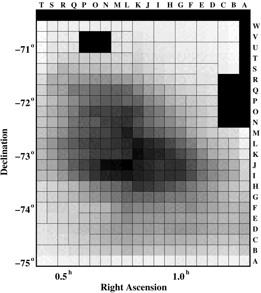
Figure 3: The division of our SMC catalog into 351 subregions. The greyscale image shows the number of stars present in our MCPS catalog from each subregion (where white means zero stars, and black means approximately 30,000 stars). The primary division imposes a uniform $20\times 23$ grid of subregions, each approximately $12\arcmin\times 12\arcmin$ in extent. Where the density of stars is very low, we combine adjacent grid cells into larger subregions. We mask some regions where foreground contamination (due to Galactic globular clusters along the line of sight) is significant. The large masked region on the west edge (regions AN through CR) is due to 47 Tucanae; the smaller masked region near the North edge is due to NGC 362.

To derive a spatially-resolved SFH, we divide the SMC Survey using a rectilinear grid of 351 subregions, as shown in Figure 3. We use a two-letter code to identify subregions by their position in the grid. The first letter identifies a subregion’s Right Ascension position in the grid, while the second letter identifies its Declination position. The letters are in alphabetical order for the direction of increasing RA or Dec. The angular size of the grid cells is a compromise between wanting small cells for finer spatial resolution in the map, and needing a large number of stars in each region for the StarFISH analysis. Some of the sparsely- populated grid cells in the outer parts of the survey region were combined into larger subregions because they did not individually contain a sufficient number of stars. Testing shows that we minimally require of order $10^{4}$ stars for a stable SFH solution. A small number of cells have been masked out and are not modeled (see Figure  3. These cells are contaminated by foreground Galactic globular clusters (the masked region near the western edge of the survey region is due to 47 Tucanae; the smaller region near the northern edge is due to NGC 362).

In addition to the goal of creating a spatially-resolved SFH map for the SMC, the division of our catalog into small regions was necessary from a practical standpoint as well. Quantitative CMD-fitting algorithms such as StarFISH depend sensitively on accurate statistical representations of both interstellar extinction and photometric errors. Since our photometric catalog covers the entirety of the SMC, it includes a wide variety of extinction and crowding conditions, making it impossible to apply these effects in a uniform way for the entire catalog. By subdividing the catalog into small regions, we account for the extinction and photometric errors locally and independently for each region, which greatly improves the correspondence between the observed photometry and the model CMD triptychs.

2.3.2 Finding the Best-Fit Model

For each of our 351 subregions, we have the $UBVI$ photometry and a library of synthetic CMD triptychs that incorporate the derived photometric errors and extinction distributions directly from the data. Given these inputs, StarFISH determines the set of amplitude values modulating each synthetic CMD triptych that produces the best fit between the observed photometry and the composite model CMD triptych by using a downhill simplex algorithm to evaluate the $\chi^{2}$ statistic of different composite models (see Harris & Zaritsky, 2001). To evaluate $\chi^{2}$, the observed and model CMD triptychs are divided onto a uniform grid with cells that are 0.25 mag wide in both the color and magnitude directions. The number of observed and model stars present in each grid cell are then compared using the standard $\chi^{2}$ formula:

$$\chi^{2}=\sum_{i}\frac{(N_{d}(i)-N_{m}(i))}{N_{d}(i)}$$

where $N_{d}(i)$ is the number of stars observed in CMD region $i$, and $N_{m}(i)$ is the number of stars in the composite model in CMD region $i$. In cases where $N_{d}(i)$ is zero (but $N_{m}(i)$ is not), the denominator is instead taken to be 1. Regions where both $N_{d}(i)$ and $N_{m}(i)$ are zero do not contribute to $\chi^{2}$. Technically, $\chi^{2}$ should only be used in the case of normally- distributed errors, which is only approximately true in our case when both $N_{d}(i)$ and $N_{m}(i)$ are large. The $\chi^{2}$ minimum can still be used to determine the best-fit model in the case of non-Gaussian errors, but one loses some ability to determine the quality of the best fit and the confidence intervals about that best-fit. Our testing of the StarFISH algorithm shows that $\chi_{\nu}^{2}\sim 1$ does provides a reasonable indication of a good fit (see  Harris & Zaritsky, 2001) for the number of stars in a typical grid cell.

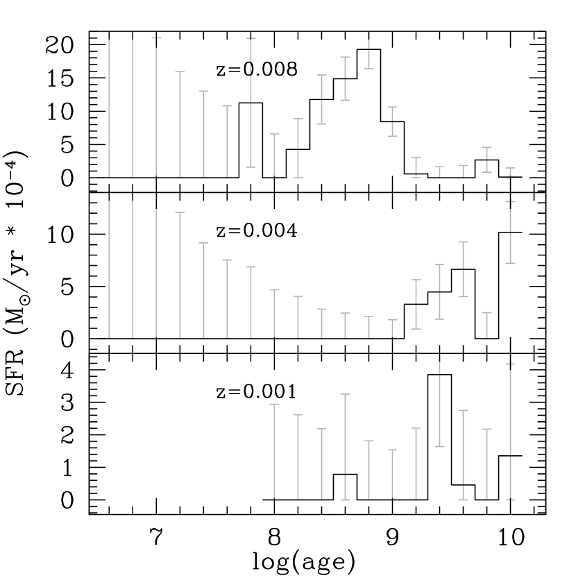
Figure 4: The SFH solution for one of our 351 regions in the SMC (the region labeled MK in Figure 3). The histogram indicates the best-fit star formation rates for 47 logarithmic age bins, across three metallicities: Z=0.008 (top panel), Z=0.004 (middle panel), and Z=0.001 (bottom panel). The errorbars represent the 1-$\sigma$ confidence interval on each amplitude, including covariance between amplitudes.

In Figure 4, we show the SFH solution for a typical region from our SMC grid (region MK). This region contained 25,848 stars, and the SFH fit solution has a reduced $\chi^{2}$ value of 3.

2.3.3 Estimating Fit Uncertainties

Once the best-fit amplitudes have been determined, the program performs a systematic exploration of the parameter space surrounding the best-fit point to determine the $1\sigma$ confidence interval on each parameter value as defined by the appropriate value of $\Delta\chi^{2}=\chi^{2}-\chi_{min}^{2}$. The exploration is performed in stages. First, each amplitude value is varied while all others are held fixed at their best-fit values. This calculation evaluates the independent uncertainty associated with each amplitude value. Second, adjacent pairs of amplitudes are varied simultaneously, while the remaining amplitudes are held fixed at their best-fit values. This evaluates the correlated errors between the adjacent amplitude pairs. Third, we perform a correlated-error analysis involving the variation of all amplitude values simultaneously. We select a random “direction” in the 47- dimensional parameter space and evaluate $\chi^{2}$ for points displaced from the best-fit point along that direction. We continue stepping away from the best-fit point until the $\Delta\chi^{2}$ value indicates that we have reached the $1\sigma$ confidence interval. The $\Delta\chi^{2}$ evaluation is repeated for 30,000 different random parameter space directions. We performed tests of the growth of the confidence intervals as the number of random directions evaluated increases. These tests show steady growth of the confidence intervals up to about 10,000 directions, and little further growth thereafter. We conclude that exploring 30,000 directions is sufficient to provide a robust determination of the correlated errors on the amplitude values. Note that without having run stages one and two first, the number of directions required for the third stage to converge would be much larger. This is because we expect each amplitude to have an independent uncertainty, and we also expect strong correlated errors between adjacent amplitudes. Relying on a random selection of directions in a 47-dimensional space to cover these particular directions would be extremely inefficient. Instead, we manually explore those directions where we expect large deviations, and use the random-direction stage to fill in any unexpected correlations.

Throughout each of the three confidence-interval stages (uncorrelated errors, pairwise correlated errors, and full correlated errors), the program keeps track of the maximum variation of each amplitude value that resulted in a $\Delta\chi^{2}$ value within the confidence interval. The final maximum variation defines the endpoints of the $1\sigma$ confidence interval assigned to each amplitude (see Figure 4 for a typical example of the SFH errors). Note that because correlated errors between amplitudes are important, the confidence-limit “error bars” are larger than the random uncertainty of the SFH solution. It can therefore be misleading to judge the significance of a fluctuation in the SFH relative to its neighboring amplitudes simply by comparing the difference in star formation rates to the plotted error bars.

2.3.4 Problem Areas

After a first-pass run of StarFISH on all 351 regions, we found that the best-fit reduced $\chi_{\nu}^{2}$ values in some regions were greater than 10. These poorly-fit regions were in the extremely crowded central parts of the SMC (see Figure 3). By adjusting which AST region we used to generate the synthetic CMD library (see Table 1), we could often improve the fit sufficiently to bring $\chi_{\nu}^{2}$ below 10. However, the need to do this manual adjustment indicates that our hypothesis that stellar surface density dominates the photometric errors does not hold true in every case.

For approximately 50 regions, the best-fit remained poor, even after trying alternate ASTs (see Figure 5). By comparing the observed CMDs in these regions to the best-fit model triptychs, it is apparent that the reason for the poor fit is a systematic color offset of 0.1–0.2 mag in $B-V$ (see Section 3.1.4 for details). It is difficult to explain this $B-V$ color excess astrophysically. If the color shift is due to extinction or a metal-rich stellar population, the $U-B$ and $V-I$ colors would have similar color excesses, but they do not. In fact, when we run StarFISH with the $B-V$ CMD excluded, the solutions have much smaller reduced $\chi^{2}$ values ($\sim 3$–4, rather than $\sim 10$). Because the $U-B$ and $V-I$ CMDs are well-fit by the models, we are reluctant to apply a $B$ or $V$ offset to correct the $B-V$ CMD (because one of the other CMDs would also be affected). For now, we empirically apply a $B-V$ correction to force the main sequence in these regions to lie coincident with the main sequence of the well-fit regions. Running StarFISH again on the problem regions after applying the empirical $B-V$ correction, the reduced $\chi_{\nu}^{2}$ values are dramatically lower, and are similar to those obtained in the rest of the map. Unless otherwise noted, we will hereafter adopt the SFH results for these regions after having applied the empirical $B-V$ correction. This correction is needed in $<$5% of the regions, does not affect the qualitative nature of the derived SFH in these regions (see Section 3.1.4), and does not affect our global conclusions.

2.3.5 Line-of-Sight Depth

Several authors have investigated the line-of-sight structure of the SMC, generally finding a measurable extension along the line-of-sight, although the depth measurements range from 10% to almost 30% of the SMC’s distance from the Milky Way. Welch et al. (1987) used 91 Cepheid variables throughout the SMC to determine a depth of $\sim 7$ kpc. Martin et al. (1989) examined distance moduli to young SMC stars, determining that their depth was $<10$ kpc. Hatzidimitriou & Hawkins (1989) and Gardiner & Hawkins (1991) used the luminosity dispersion of the red clump to infer depths as large as 17 kpc in the outer regions of the SMC (although perhaps half as large as this in many regions). More recently, Groenewegen (2000) cross-referenced hundreds of cepheids in the OGLE, DENIS, and 2MASS surveys, finding a depth of 14 kpc; while Crowl et al. (2001) used SMC star clusters to determine a depth of 6–12 kpc.

To test whether we need to account for line-of-sight depth in our analysis, we assume a characteristic depth of 12 kpc, corresponding to $\pm 0.2$ mag in distance modulus. We constructed artificial stellar populations with this intrinsic luminosity spread, and performed the StarFISH analysis without accounting for the spread in distance. The $\chi^{2}$ value of the solution is slightly inflated compared to an identical zero-depth population, but the SFH solutions were the same, within the errors. In addition, we see no empirical evidence in the zero-depth model fits to the real data that a significant line-of-sight depth is required, so we omit it in the present analysis.

2.4 Results: A Map of the SMC’s Star Formation History

In Table 2, we present our best SFH solutions for 351 regions in the SMC. The SFH amplitudes output by StarFISH are equal to the number of stars which were formed in each age/metallicity bin. In the Table (and in all subsequent discussion), the SFH amplitudes have been converted to star-formation rates by simply multiplying by the IMF-dependent mean stellar mass, and dividing by the age interval covered by the bin. This is straightforward for all bins except the oldest, for which we have only a lower age limit. We adopt an upper age limit of 13.7 Gyr in computing the star-formation rates of the oldest bin.

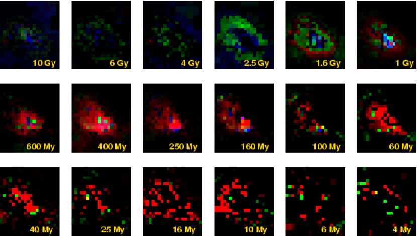
Figure 6: The star-formation history of the SMC. Each panel shows the star formation activity for a particular age bin; the characteristic age of the bin is labeled. Each pixel represents one of our 351 SMC subregions (see Figure 3), with a pixel value that is proportional to the subregion’s star formation rate (in the electronic edition, the pixels are also color-coded to reflect the mean metallicity of the stars. Red corresponds to Z=0.008, green corresponds to Z=0.004, and blue corresponds to Z=0.001).

The information presented in Table 2 is condensed into a map of the SMC’s star-formation history in Figure 6. Each panel in the Figure represents a “snapshot” of the star- formation activity at a particular epoch. In each panel, the 351 subregions are represented as “pixels” of variable size whose brightness is proportional to the local star-formation rate (SFR). The SFH map is available as an animation at [URL to be specified].

3 Discussion

3.1 The Global Star Formation History

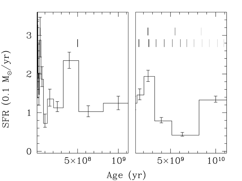
Figure 7: The global star formation history of the SMC. We sum the star formation rates across metallicity and the 351 individual subregions. We use a split-panel view with different scalings of the time axis because the age bins become logarithmically narrower for younger ages. The displayed error bars represent the 1-$\sigma$ confidence interval for each age bin and include covariance between age bins. The times at which the SMC had a perigalactic passage are indicated by the rows of short vertical lines (Lin et al., 1995). The top row indicates encounters with the LMC, the bottom row indicates encounters with the Milky Way. These lines fade out at older ages as a representation of the uncertainty of the encounter times with increasing age.

In Figure 7, we show the global SFH of the SMC, derived by summing together the star-formation rates over all 351 subregions and over all three metallicities. The SFH revealed by Figures 6 and 7 contains several interesting features: (1) there was a significant epoch of star formation in our oldest age bin, covering all ages older than 8.4 Gyr, (2) there was a long quiescent epoch between 3 and 8.4 Gyr ago, during which the SMC apparently formed relatively few stars, (3) the quiescent epoch was followed by more-or-less continuous star formation starting about 3 Gyr ago, and extending to the present, (4) superimposed on the recent continuous star formation, there are at least three peaks in the SFR, at 2–3 Gyr, 400 Myr and 60 Myr ago, and (5) there is a ring-like morphology in the intermediate-age frames (2.5–1.0 Gyr) that may suggest an inward propagation of star formation or the remnant of a gas-rich merger event.

3.1.1 The First Stars

Although it is difficult to discern any details about the SFH at the earliest times, the determination that a large fraction of all stars in the SMC correspond to a population from the earliest times is critical. We find that the SMC formed about 50% of its total stellar population prior to 8.4 Gyr ago, or alternatively at $z>1.2$ for WMAP cosmology (Spergel et al., 2003). Like all Local Group systems (Mateo, 1998), the SMC contains a significant old population.

It is useful to compare our results for the early history of the SMC to previous work in this area. Gardiner & Hatzidimitriou (1992) found that the bulk of the SMC’s stars are aged $\sim 10$ Gyr; while they didn’t offer a quantitative fraction, from their discussion it can be inferred that the number is substantially larger than 50%. However, this difference may be attributed to the fact that Gardiner & Hatzidimitriou studied the outer portions of the SMC where the younger stellar populations are probably much less common.

More recently, Dolphin et al. (2001) used a deep HST WFPC2 field near NGC 121 to reconstruct the old SFH of the SMC. The deep HST photometry includes stars well below the ancient main sequence turn-off, so it is a superior data set for reconstructing the early history of the SMC in this regard. Dolphin et al. find a SFH which peaks between 5 and 8 Gyr ago, in contrast to what we find. However, there are two factors which make direct comparisons of the two solutions difficult. First, our analysis regions do not overlap; they used a field near NGC 121, which falls within the region we masked out to avoid contamination from the foreground galactic cluster 47 Tucanae. Second, the Dolphin et al. field is well outside the main portion of the SMC, so it would seem dangerous to infer a general SFH for the entire SMC based on this small field at its periphery. Still, one could argue against both of these explanations by pointing out that for the old SFH at least, the stellar populations should be well-mixed, so even a tiny sample should be representative of the whole. Part of the problem may be the coarser age resolution employed in our analysis (as mandated by our ground-based data). More deep-field SFH analyses from different regions in the SMC should be performed to investigate the issue.

3.1.2 The Quiescent Epoch

The second and third panels of Figure 6 are globally dark, indicating an epoch lasting several Gyr during which the SMC formed relatively few stars. To ensure that the lack of detected star formation in these panels is not an artifact of our method, we added supplemetary synthetic stellar populations to several selected SMC regions. The supplemental populations have the correct number and age distribution (3–8.4 Gyr) to fill in the apparent age gap in the observed SFH. We found that the StarFISH algorithm successfully recovered the “observed + synthetic” star formation history, indicating that the method is not inherently insensitive to stellar populations in this age range.

The quiescent epoch we infer from the SMC’s field stars is intriguingly coincident with the well-known “age gap” among star clusters in the Large Magellanic Cloud (van den Bergh, 1991; Da Costa, 1991; Girardi et al., 1995; Westerlund, 1997). Although the cluster population in the SMC has been conventionally regarded as having a continuous age distribution (Da Costa & Hatzidimitriou, 1998; Mighell et al., 1998), analysis of deep Hubble Space Telescope photometry of the SMC’s seven brightest old (age $>1$ Gyr) clusters (Rich et al., 2000) has shown that most of the SMC’s old clusters were formed in two sharply distinct episodes: one that occurred $8\pm 2$ Gyr ago and one that occurred $2\pm 0.5$ Gyr ago. Furthermore, Rich et al. discuss three SMC clusters that are too faint to be included in their $HST$ study. One (Lindsay 1) has a ground-based age of 9 Gyr, coincident with the older burst. The other two have ground-based ages between the 2 and 8 Gyr bursts (Lindsay 11 has an age of 3.7 Gyr and Lindsay 113 has an age of 6 Gyr). The age of Lindsay 113 was confirmed by Crowl et al. (2001), who used ground-based photometry to derive an age of $5.3\pm 1.3$ Gyr. Therefore, our present understanding is that among the SMC’s ten populous old clusters, eight were formed in one of two epsiodes, and two were formed at some time between the episodes. While the number of SMC clusters is small, their age distribution is not uniform and is qualitatively consistent with our SFH derived from the SMC’s field population. In a subsequent paper, we will present an analysis of the ages of 204 SMC stellar clusters that independently confirm the quiescent epoch seen here among the stars, as well as the bursts discussed next.

3.1.3 “Bursts” of Star Formation

From Figure 7, the SFH since 3 Gyr ago can be characterized as having an underlying constant SFR of $\sim 0.1\ M_{\odot}\ yr^{-1}$ with superimposed episodes of enhanced star formation at 2–3 Gyr, 400 Myr, and 60 Myr. The mean SFR in these age bins is a factor of 2–3 times higher than in the surrounding bins.

We hesitate to conclude that the SMC has had exactly three bursts in its history, because rapid star-formation events can happen on timescales that are orders of magnitude shorter than synthetic CMD methods are able to resolve, especially at ages $\mathrel{\hbox{\raise 2.15277pt\hbox{$>$}\hbox to0.0pt{\hss\lower 2.15277pt\hbox{$\sim$}}}}1$ Gyr. The actual star formation rate as a function of time could be varying wildly within any of our age bins, and we would not know it. We only measure the mean star formation rate over the width of the bin. It is certainly possible that these enhanced star-formation events were dominated by a multiple, distinct, short-duration burst, which were each much stronger than the 2–3$\times$ enhancement reflected in the mean star formation rate. Similarly, we do not intend to imply that we have actually observed a more-or-less constant inter-burst SFR in the SMC over the past 3 Gyr; the unknowable possibility of short-term SFR variations prevents such a conclusion. We simply characterize the observed SFH as having a baseline constant SFR in order to highlight the three superimposed episodes of heightened star formation.

Figure 7 indicates 5 times at which the SMC had a perigalactic encounter with the Milky Way, and 14 perigalactic encounters with the LMC, over the past 12 Gyr (Lin et al., 1995). In addition, the SMC is believed to be currently very near perigalacticon with respect to the Milky Way. The most recent perigalactic encounters ($\sim 500$ Myr ago for the LMC, $\sim 2.5$ Gyr ago for the Milky Way) fall in the age bins in which we have observed significantly enhanced star formation rates, raising the possibility that we have recorded the effects of interaction-induced star formation in the SMC. For the older encounters, we lack the age resolution to discern any response in the SMC’s SFH to these short-lived events. These issues are explored in greater detail in a companion paper (Zaritsky & Harris, 2004).

3.1.4 A Ring of Star Formation?

There is unexpected large-scale spatial structure in the SFH map (Figure 6) at intermediate ages (2.5 to 1 Gyr). Naively, one might expect stellar populations of this age to be well-mixed and that their distribution would follow the overall stellar density (see Figure 3). The ring is most prominent in the 2.5 Gyr frame, where the dense central regions are almost totally quiescent, and the encircling ring is highly active, especially to the northeast. In the 1.6 Gyr frame, there is some low-metallicity star formation activity in the central regions, and the active ring regions have become more metal rich. Starting with the 1 Gyr frame, the distribution of SFRs is finally centrally peaked as one would expect, but the activity in the central regions is still of lower metallicity than in the encircling ring.

Before we attempt to interpret this structure, we must determine whether it is an artifact in the data or of the analysis. There are three reasons to suspect that the ring may not be real. First, the shape of the ring approximately follows the stellar surface density contours in the SMC. If our method is subtly sensitive to errors in the modeling of the stellar crowding, we might expect to see recovered age discrepancies proportional to the projected stellar density, which could result in a ring-like artifact in the SFH map. Second, and perhaps related to the first point, the regions that form the “hole” interior to the ring feature are the same regions which required a modest $B-V$ color offset for us to obtain an acceptable SFH model. Third, the synthetic CMDs corresponding to the age range where the ring is most prominent have their main-sequence turn offs at the faint end of the CMD, where the completeness rate and photometric errors change rapidly as a function of magnitude and are most difficult to model.

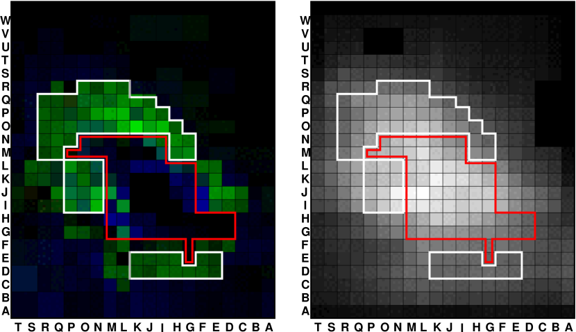
Figure 8: The left panel shows the 2.5 Gyr frame of our SFH map (Figure 6), the right panel shows the star counts in each subregion (Figure 3). We highlight the 68 regions that we combine into an “on” population, based on their star formation rate at 2.5 Gyr (solid white outline). We also highlight the 68 regions that we combine into an “off” population (dashed outline; or red outline in the electronic edition). These two composite populations are compared to investigate the nature of the ring-like structure visible in the 2.5 Gyr map frame.

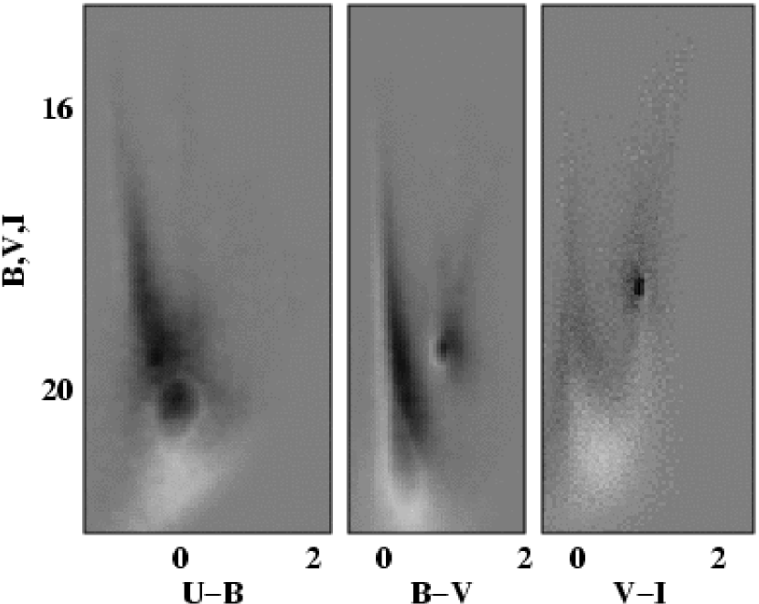
Figure 9: CMD triptych showing the difference between the “on” and “off” meta-regions. White pixels indicate an excess of stars among the “on” population; black pixels indicate an excess of stars among the “off” population. The “on” population has an excess of faint main-sequence stars, compared to the “off” population, and there is a systematic offset in the $B-V$ color of the two populations.

To understand which features in the CMDs are driving the dramatic contrast between the active and quiescent regions which form the ring at 2.5 Gyr, we use the 2.5 Gyr SFH frame of Figure 6 to isolate and compare two stellar populations: an “on” population drawn from the active regions within the ring, and an “off” population drawn from the quiescent central regions (see Figure 8). CMD triptychs for these composite regions, as well as the difference between them, are shown in Figure 9. These CMDs show the original photometry, without the applied $B-V$ offset that was used in determining the SFHs (see Section 2.3.4).

The most prominent feature of the difference CMDs is an excess of faint main sequence stars in the “on” regions relative to the “off” regions. Because the central regions are also generally the most crowded, this difference can be regarded as the expected result of a brighter faint limit in the more crowded regions. Although this difference should not affect the best-fit SFHs if our ASTs are correct, it is suspicious that that this difference lies precisely where the main sequence turn-off stars of a 2–3 Gyr population would be found. Overestimating the faint-end completeness rate in the central regions would result in a suppressed formation rate at 2–3 Gyr, similar to that observed in the central regions.

If the deficit of faint main sequence stars is the explanation for the suppresed star formation in “off” regions, we must understand why the ASTs failed to produce a viable model of the completeness rate in these regions. The problem cannot simply be due to higher stellar surface densities of the “off” regions because there are “on” regions which have similarly high stellar surface densities (see Figure 8). If there is an AST failure, it is more likely caused by our assumption that crowding effects dominate the photometric errors; in other words, there may be non-crowding parameters affecting the photometry of the “off” regions. This will skew our results if the SFH solution uses a synthetic CMD library based on ASTs from an image which is not an “off” region. However, even this cannot be the right answer, because we are in fact using ASTs derived from “off” regions to construct their synthetic CMD libraries. In particular, we use ASTs from regions JJ and KK, so at the very least, these two regions must have photometric error characteristics that are appropriately described by the adopted ASTs. Yet regions JJ and KK are unequivocally among the “off” regions. We find no reason to believe that these AST results are in error.

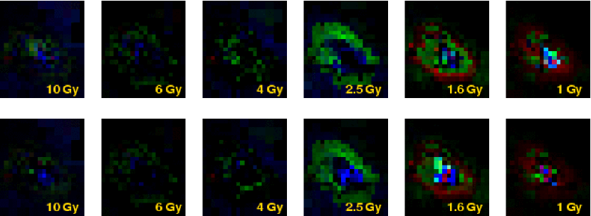
Figure 10: Comparing the oldest six bins of the SFH map, with and without the $B-V$ color offset. Top row: the original solution, in which we applied a $B-V$ offset to some of the subregions, in order to improve the $\chi^{2}$ values of our SFH solutions (see Section 2.3.4). Bottom row: An alternate solution, in which we did not apply color offsets to any subregions.

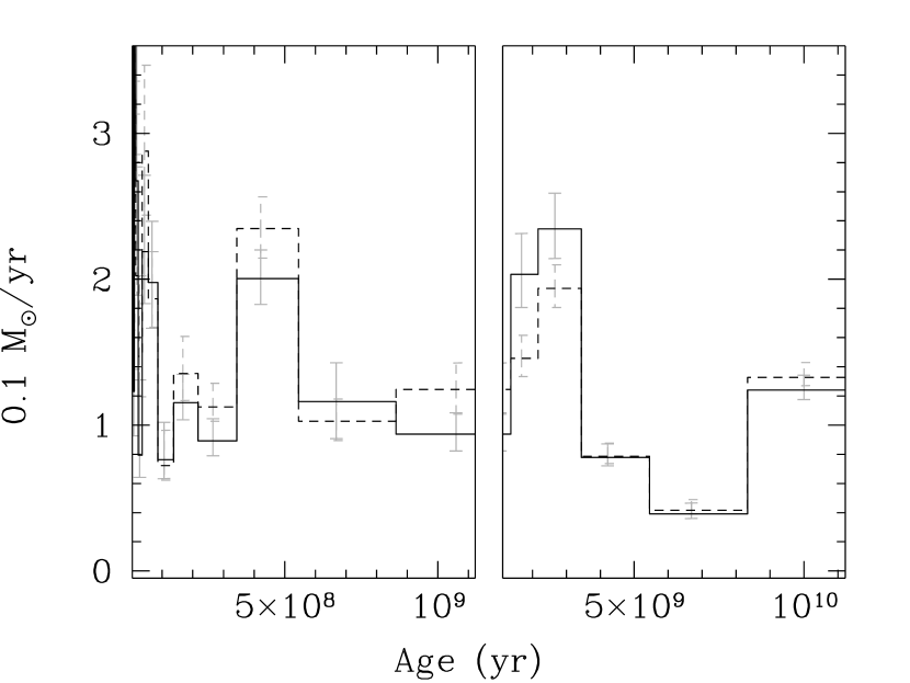
Figure 11: Comparing the global SFH solution, with and without the $B-V$ color offset. The original SFH solution from Figure 7 is shown as the solid histogram. This solution included a $B-V$ color offset applied to the photometry of some subregions to improve the $\chi^{2}$ of their SFH solutions. The dotted histogram shows an alternate SFH solution, for which no $B-V$ color offsets were applied. There is no significant difference between the two solutions.

Another notable feature visible in the difference CMDs of Figure 9 is the displacement of the main sequence in the $B-V$ CMD, in the sense that the main sequence in the “off” regions is systematically redder than that of the “on” regions. The most plausible explanation seems to be a systematic photometric zeropoint offset in the photometry of these central regions, which motivated us to apply a $B-V$ correction to improve their best-fit SFHs (see Section 2.3.4). However, since the cause of this offset is unknown, we must suspect the SFH solutions for these regions. We investigate the effect of the $B-V$ color correction on the SFHs of the “off” regions by comparing the SFH solutions including the $B-V$ correction to a second set of SFH solutions in which the $B-V$ correction was not applied (see Figure 10). The “hole” is less prominent when no color offset is applied, but it is still present, and there is still a strong radial trend in metallicity. In Figure 11, we compare the global SFH solutions for the cases with and without the applied $B-V$ offset. This Figure shows that the application of the $B-V$ offset to the central subregions has very little effect on our overall SFH solution for the SMC. Because the $\chi^{2}$ values are substantially improved when the $B-V$ offset is applied, we retain our original SFH solutions, which include the offset. The nature of the $B-V$ offset remains a mystery and so the SFH of the central regions must be viewed with caution. Further understanding of these apparently anomalous main sequence populations may require deeper photometry with large ground-based telescopes or with the $HST$.

If the observed ring feature is real, it suggests the possibility of a global inward propagation of star formation in the SMC on a timescale of a few Gyr. Alternatively, the ring may be composed of stars that formed as the result of a gas-rich merger 2–3 Gyr ago. The latter is consistent with an infall scenario that reproduces the SMC’s chemical enrichment history (Zaritsky & Harris (2004)) and the different distribution of young and old stars in the SMC Zaritsky et al. (2000). In this scenario, the kinematics of the stellar population formed by the merger would follow the kinematics of the infalling gas; the gas kinematics might have sufficient angular momentum to produce stellar populations in a persistent annular distribution. Kinematic measurements of different populations in the SMC might test this scenario.

3.2 The Chemical Enrichment History

Previous analyses of the chemical enrichment history (CEH) of the SMC, based primarily on measurements of $\sim 10$ stellar clusters in the SMC (Dopita, 1991), have noted very little change in the metallicity of clusters between 10 and 4 Gyr old. To explain this observation, investigators have invoked either significant infall of unenriched gas or a “leaky box” model, in which supernova-driven winds preferentially remove heavy elements. However, Da Costa & Hatzidimitriou (1998) re-examined the cluster data, and concluded that if two “anomalous” clusters are ignored, the age-metallicity relation increases gradually and monotonically, consistent with a simple closed-box enrichment model. Pagel & Tautvaisienė (1999) again examined the cluster data and concluded, in agreement with Dopita (1991), that the metallicity in the SMC remained low until $\sim 4$ Gyr ago. Pagel & Tautvaisienė present a simple chemical enrichment model consistent with the cluster data, in which the long period of stagnant enrichment between 4 and 10 Gyr is explained by a lull in the star formation rate over the same period. We note that we have observed a very similar lull in the star formation rate among the SMC’s field populations (see Figure 7 and Section 3.1.2).

In addition to the work on star clusters, field variable stars have also provided some constraint on the CEH of the SMC. Smith et al. (1992) inferred from the period-amplitude relation that the metallicity of RR Lyrae stars in the SMC is similar to that of the field giants of Suntzeff et al. (1986); [Fe/H]=-1.6. Butler et al. (1982) measured the metallicities of three field RR Lyrae stars directly from spectra, finding $<[Fe/H]>=-1.8$ for these old stars. In addition, Harris (1981) measured photometric abundances of 45 Cepheid variables in the SMC, finding $<[Fe/H]>=-0.5$ for these intermediate-age ($\sim 10^{8}$ yr) populations.

Our recovery of the SMC’s SFH provides an independent determination of its CEH. Before beginning the SFH analysis, we suspected that we might have to impose a priori constraints on the CEH, since stellar photometry allows only crude measurements of metallicity. Instead, we found that StarFISH was able to converge upon a reasonable CEH without a priori constraints.

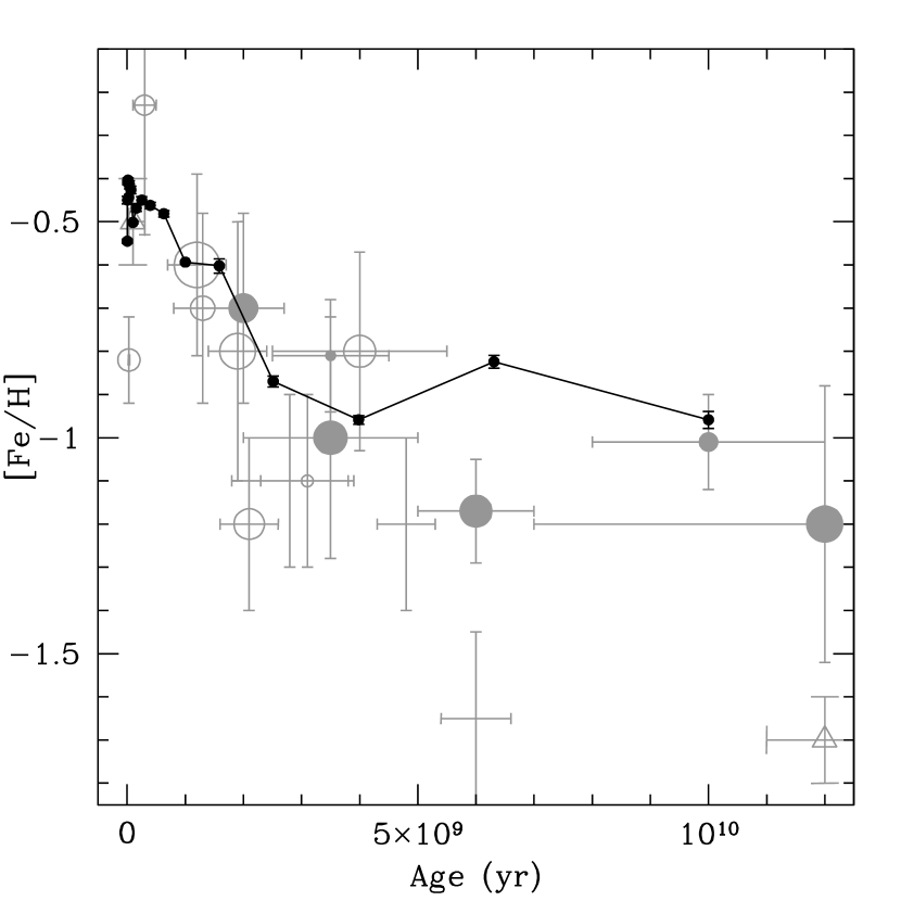
Figure 12: The age-metallicity relation derived from our SFH analysis is shown as the small points connected with straight-line segments. The grey points represent existing metallicity and age measurements in the literature. Circular points represent star clusters, and the size of each circle is proportional to the cluster’s estimated mass (some circles are too small to be seen in the Figure). The six solid circles represent the clusters used by Dopita (1991), Da Costa & Hatzidimitriou (1998) and Pagel & Tautvaisienė (1999), and the open circles are from de Freitas Pacheco et al. (1998) and Piatti et al. (2001). The triangular point at 11 Gyr represents the field RR Lyrae stars as measured by Smith et al. (1992) and Butler et al. (1982), and the triangular point at 0.1 Gyr represents the field Cepheid stars, as measured by Harris (1981).

To quantify the CEH, we determine the mean metallicity of stars formed at a given age, and plot this as a function of age in Figure 12. We convert from $Z$ metallicities to $[Fe/H]$ values by adopting $Z_{\odot}=0.02$, and assuming that $[Fe/H]=log(\frac{Z}{Z_{\odot}})$. The error bars on our age-metallicity relation (AMR) represent the standard deviation of the individual subregions’ metallicity values about the global mean metallicity in each age bin, and do not necessarily reflect the precision with which we have determined the mean metallicity.

We find that our AMR agrees quite well with the star cluster and field variable data, even though our photometrically-derived metallicities are necessarily crude. We find that the field metallicity in the SMC remained rather low ($[Fe/H]\sim-1.0$) until 2–3 Gyr ago, at which point it began a steady increase to its present-day value of $[Fe/H]\sim-0.5$. There is a marginal indication that the mean metallicity actually decreased between 7 and 4 Gyr ago. Our derived CEH is consistent with the chemical enrichment model of Pagel & Tautvaisienė (1999), lending further support to the presence of a quiescent epoch in the SMC’s early history. The implications of the CEH in the context of the SMC’s interaction history is discussed in detail in a subsequent paper (Zaritsky & Harris, 2004).

4 Summary

From the reconstruction of $UBVI$ color-magnitude diagrams using the StarFISH Harris & Zaritsky (2001) analysis package and comparison to the MCPS $UBVI$ photometry of stars in the SMC Zaritsky et al. (2002), we determine the global star formation history as resolved on a grid of 351 independent subregions. Critical components of this analysis include differential reddening that accounts for both spatial and population dependencies, and extensive artificial star tests to determine the photometric error model and completeness correction.

We find that the recovered SFH of the SMC can be divided into three epochs:

1) An early epoch ($t>8.4$ Gyr ago) where a significant fraction ($\sim 50$%) of all stars in the SMC were formed. Because we have poor temporal resolution at these early times, we can only constrain the total number of stars older than 8.4 Gyr, and not a more detailed distribution of their ages.

2) An intermediate epoch ($3<t<8.4$ Gyr) where the SMC experienced a long quiescent period during which it formed relatively few stars. This quiescent time parallels the lack of known clusters of these ages both in the LMC and SMC.

3) An active recent time ($t<3$ Gyr) where there has been continuous star formation punctuated by “bursts” at 2.5 Gyr, 400 Myr and 60 Myr. The older two events are coincident with past perigalactic passages by the SMC with the Milky Way. The strongest burst, that at 2.5 Gyr, appears to have an annular structure and an inward propagation spanning $\sim 1$ Gyr. However, we remain skeptical about the reality of this structure, and deeper photometry of the SMC’s crowded central regions is required to investigate further.

For our derived chemical enrichment history we find:

1) that the mean chemical abundance of stars formed in the SMC remains low ($[Fe/H]\sim-1$) until about 3 Gyr ago and then rises monotonically to the present gas-phase abundance value of $[Fe/H]\sim-0.4$].

2) that our observed AMR is consistent with existing age and metallicity measurements of populous star clusters in the SMC.

3) that our relation is inconsistent with a simple closed-box enrichment model, unless the quiescent epoch we have observed was nearly devoid of significant star formation.

Because of the decreasing temporal resolution with lookback time, it is not straightforward to infer the detailed behavior of the star formation rate from the reconstructed SFH. Instead, models must be convolved with the binning structure imposed by the method. In a companion paper Zaritsky & Harris (2004) we address whether the SFH and chemical enrichment history is consistent with a model where pericenter passages drive star formation. Both the SFH and chemical enrichment history are sufficiently complex and rich in behavior that we hold out hope that they may be able to provide interesting constraints on the nature of star formation in galaxies.

Acknowledgements: DZ acknowledges financial support from National Science Foundation CAREER grant AST-9733111 and a fellowship from the David and Lucile Packard Foundation.

Figure 2: The measured extinction distributions from eight selected SMC subregions. Each panel shows both the cool-star sample (open histogram) and the hot-star sample (shaded histogram) for stellar populations drawn from that particular SMC subregion. The subregion is identified by the two-letter code in the top-right corner of each panel (see Figure 3). The subregions were selected to illustrate the spatial variation in the extinction properties of the SMC. While the cool-star extinction distributions are rather uniform throughout the SMC, the hot-star extinction distributions vary substantially. In addition, the hot-star and cool-star distributions are always much wider than the measurement errors, making it inadvisable to characterize the extinction in any region of the SMC with a single value.

Table 1: The Artificial Stars Tests

Subregion	$N_{\star}/\Box\arcmin$	Subregion	$N_{\star}/\Box\arcmin$
TM	57.4	MO	176.6
RM	104.5	MM	186.4
PM	152.1	JJ	197.6
PO	153.5	KK	221.6

Table 2: The Star Formation History of the SMC

Age Range	Z = 0.008			Z = 0.004			Z = 0.001
log(yr)	$SFR$	$SFR_{low}$	$SFR_{high}$	$SFR$	$SFR_{low}$	$SFR_{high}$	$SFR$	$SFR_{low}$	$SFR_{high}$
Region AA ( 0h 25m, -74° 57′)
9.925–10.05	0	0	29	0	0	42	416	306	526
9.725–9.925	0	0	23	0	0	32	37	0	120
9.525–9.725	0	0	23	0	0	42	0	0	100
9.325–9.525	0	0	29	0	0	61	331	246	416
9.125–9.325	0	0	48	106	32	180	0	0	61
8.925–9.125	0	0	43	0	0	56	0	0	48
8.725–8.925	0	0	50	0	0	52	0	0	53
8.525–8.725	55	0	109	0	0	50	0	0	53
8.325–8.525	0	0	57	0	0	62	0	0	64
8.125–8.325	0	0	80	0	0	80	0	0	86
7.925–8.125	0	0	110	0	0	110	0	0	120
7.725–7.925	0	0	180	0	0	180	$\cdots$	$\cdots$	$\cdots$
7.525–7.725	0	0	230	0	0	240	$\cdots$	$\cdots$	$\cdots$
7.325–7.525	0	0	360	0	0	370	$\cdots$	$\cdots$	$\cdots$
7.125–7.325	0	0	560	145	5	725	$\cdots$	$\cdots$	$\cdots$
6.925–7.125	0	0	900	0	0	890	$\cdots$	$\cdots$	$\cdots$
6.725–6.925	0	0	1400	0	0	1500	$\cdots$	$\cdots$	$\cdots$
6.600–6.725	0	0	2600	0	0	2900	$\cdots$	$\cdots$	$\cdots$

Note. — The complete version of this table is in the electronic edition of the Journal. The printed edition contains only a sample.

References

- Ardeberg et al. (1997) Ardeberg, A., Gustafsson, B., Linde, P., & Nissen, P. E. 1997, A&A, 322, L13
- Butler et al. (1982) Butler, D., Demarque, P., & Smith, H. A. 1982, ApJ, 257, 592
- Crowl et al. (2001) Crowl, H. H., Sarajedini, A., Piatti, A. E., Geisler, D., Bica, E., Clariá, J. J., & Santos, J. F. C. 2001, AJ, 122, 220
- Cutri & McAlary (1985) Cutri, R. M. & McAlary, C. W. 1985, ApJ, 296, 90
- Da Costa (1991) Da Costa, G. S. 1991, in IAU Symp. 148: The Magellanic Clouds, 183–+
- Da Costa & Hatzidimitriou (1998) Da Costa, G. S. & Hatzidimitriou, D. 1998, AJ, 115, 1934
- de Freitas Pacheco et al. (1998) de Freitas Pacheco, J. A., Barbuy, B., & Idiart, T. 1998, A&A, 332, 19
- Dolphin et al. (2001) Dolphin, A. E., Walker, A. R., Hodge, P. W., Mateo, M., Olszewski, E. W., Schommer, R. A., & Suntzeff, N. B. 2001, ApJ, 562, 303
- Dopita (1991) Dopita, M. A. 1991, in IAU Symp. 148: The Magellanic Clouds, Vol. 148, 393+
- Duquennoy & Mayor (1991) Duquennoy, A. & Mayor, M. 1991, A&A, 248, 485
- Gallagher et al. (1996) Gallagher, J. S., Mould, J. R., de Feijter, E., Holtzman, J., Stappers, B., Watson, A., Trauger, J., Ballester, G. E., Burrows, C. J., Casertano, S., Clarke, J. T., Crisp, D., Griffiths, R. E., Hester, J. J., Hoessel, J., Krist, J., Matthews, L. D., Scowen, P. A., Stapelfeld, K. R., & Westphal, J. A. 1996, ApJ, 466, 732
- Gardiner & Hatzidimitriou (1992) Gardiner, L. T. & Hatzidimitriou, D. 1992, MNRAS, 257, 195
- Gardiner & Hawkins (1991) Gardiner, L. T. & Hawkins, M. R. S. 1991, MNRAS, 251, 174
- Girardi et al. (2002) Girardi, L., Bertelli, G., Bressan, A., Chiosi, C., Groenewegen, M. A. T., Marigo, P., Salasnich, B., & Weiss, A. 2002, A&A, 391, 195
- Girardi et al. (1995) Girardi, L., Chiosi, C., Bertelli, G., & Bressan, A. 1995, A&A, 298, 87
- Groenewegen (2000) Groenewegen, M. A. T. 2000, A&A, 363, 901
- Harris (1981) Harris, H. C. 1981, AJ, 86, 1192
- Harris & Zaritsky (1999) Harris, J. & Zaritsky, D. 1999, AJ, 117, 2831
- Harris & Zaritsky (2001) —. 2001, ApJS, 136, 25
- Hatzidimitriou & Hawkins (1989) Hatzidimitriou, D. & Hawkins, M. R. S. 1989, MNRAS, 241, 667
- Holtzman et al. (1999) Holtzman, J. A., Gallagher, J. S., I., Cole, A. A., Mould, J. R., Grillmair, C. J., Ballester, G. E., Burrows, C. J., Clarke, J. T., Crisp, D., Evans, R. W., Griffiths, R. E., Hester, J. J., Hoessel, J. G., Scowen, P. A., Stapelfeldt, K. R., Trauger, J. T., & Watson, A. M. 1999, AJ, 118, 2262
- Larson & Tinsley (1978) Larson, R. B. & Tinsley, B. M. 1978, ApJ, 219, 46
- Lin et al. (1995) Lin, D. N. C., Jones, B. F., & Klemola, A. R. 1995, ApJ, 439, 652
- Lonsdale et al. (1984) Lonsdale, C. J., Persson, S. E., & Matthews, K. 1984, ApJ, 287, 95
- Martin et al. (1989) Martin, N., Maurice, E., & Lequeux, J. 1989, A&A, 215, 219
- Mateo (1998) Mateo, M. L. 1998, ARA&A, 36, 435
- Mighell et al. (1998) Mighell, K. J., Sarajedini, A., & French, R. S. 1998, AJ, 116, 2395
- Olsen (1999) Olsen, K. A. G. 1999, AJ, 117, 2244
- Pagel & Tautvaisienė (1999) Pagel, B. E. J. & Tautvaisienė, G. 1999, Ap&SS, 265, 461
- Piatti et al. (2001) Piatti, A. E., Santos, J. F. C., Clariá, J. J., Bica, E., Sarajedini, A., & Geisler, D. 2001, MNRAS, 325, 792
- Rich et al. (2000) Rich, R. M., Shara, M., Fall, S. M., & Zurek, D. 2000, AJ, 119, 197
- Sirianni et al. (2002) Sirianni, M., Nota, A., De Marchi, G., Leitherer, C., & Clampin, M. 2002, ApJ, 579, 275
- Smecker-Hane et al. (2002) Smecker-Hane, T. A., Cole, A. A., Gallagher, J. S., & Stetson, P. B. 2002, ApJ, 566, 239
- Smith et al. (1992) Smith, H. A., Silbermann, N. A., Baird, S. R., & Graham, J. A. 1992, AJ, 104, 1430
- Spergel et al. (2003) Spergel, D. N., Verde, L., Peiris, H. V., Komatsu, E., Nolta, M. R., Bennett, C. L., Halpern, M., Hinshaw, G., Jarosik, N., Kogut, A., Limon, M., Meyer, S. S., Page, L., Tucker, G. S., Weiland, J. L., Wollack, E., & Wright, E. L. 2003, ApJS, 148, 175
- Stetson (1987) Stetson, P. B. 1987, PASP, 99, 191
- Suntzeff et al. (1986) Suntzeff, N. B., Friel, E., Klemola, A., Kraft, R. P., & Graham, J. A. 1986, AJ, 91, 275
- Tody (1986) Tody, D. 1986, in Instrumentation in astronomy VI; Proceedings of the Meeting, Tucson, AZ, Mar. 4-8, 1986. Part 2 (A87-36376 15-35). Bellingham, WA, Society of Photo-Optical Instrumentation Engineers, 1986, p. 733., 733–+
- van den Bergh (1991) van den Bergh, S. 1991, ApJ, 369, 1
- Welch et al. (1987) Welch, D. L., McLaren, R. A., Madore, B. F., & McAlary, C. W. 1987, ApJ, 321, 162
- Westerlund (1997) Westerlund, B. E. 1997, ”The Magellanic Clouds” (Book,)
- Zaritsky (1999) Zaritsky, D. 1999, AJ, 118, 2824
- Zaritsky & Harris (2004) Zaritsky, D. & Harris, J. 2004, accepted to AJ
- Zaritsky et al. (2000) Zaritsky, D., Harris, J., Grebel, E. K., & Thompson, I. B. 2000, ApJ, 534, L53
- Zaritsky et al. (1997) Zaritsky, D., Harris, J., & Thompson, I. 1997, AJ, 114, 1002
- Zaritsky et al. (2002) Zaritsky, D., Harris, J., Thompson, I. B., Grebel, E. K., & Massey, P. 2002, AJ, 123, 855
- Zaritsky et al. (1996) Zaritsky, D., Schectman, S. A., & Bredthauer, G. 1996, PASP, 108, 104