The Three-point Correlation Function of Galaxies Determined from the 2dF Galaxy Redshift Survey

Abstract

In a detailed analysis of the three point correlation function (3PCF) for the 2dF Galaxy Redshift Survey we have accurately measured the 3PCF for galaxies of different luminosity. The 3PCF amplitudes [$Q_{red}(s,u,v)$ or $Q_{proj}(r_{p},u,v)$] of the galaxies generally decrease with increasing triangle size and increase with the shape parameter $v$, in qualitative agreement with the predictions for the clustering of dark matter in popular hierarchical CDM models. The 2dFGRS results agree well with the results of Jing & Börner for the Las Camapanas Redshift Survey (LCRS), though the measurement accuracy is greatly improved in the present study because the 2dFGRS survey is much larger in size than the LCRS survey. The dependence of the 3PCF on luminosity is not significant, but there seems to be a trend for the brightest galaxy sample to have a lower amplitude than the fainter ones.

Comparing the measured 3PCF amplitudes [$Q_{red}(s,u,v)$ or $Q_{proj}(r_{p},u,v)$] to the prediction of a WMAP concordance model, we find that the measured values are consistently lower than the predicted ones for dark matter. This is most pronounced for the brightest galaxies (Sample I), for which about one-half of the predicted $Q$ value provides a good description of $Q_{proj}(r_{p},u,v)$ for the 2dFGRS data. For the less luminous sample (Sample II), the $Q$ values are also smaller than in the dark matter model on small scales, but on scales larger than $s=8\,h^{-1}{\rm{Mpc}}$ and $r_{p}=3.25\,h^{-1}{\rm{Mpc}}$ they reach the model values. Therefore, the galaxies of sample II are unbiased tracers on linear scales, but the bright galaxies (sample I) have a linear bias factor of $\sim 1.5$. As for the LCRS data, we may state that the best fit DM model gives higher values for the 3PCF than observed. This indicates that the simple DM models must be refined, either by using more sophisticated bias models, or a more sophisticated combination of model parameters.

1 Introduction

To infer the spatial distribution of cosmic matter from the observed distribution of galaxies is a nontrivial task. Big redshift catalogs of galaxies, and numerical simulations of the dark matter clustering depending on the cosmological model and on initial conditions, are the observational and theoretical basis for a treatment of this problem. The statistical properties, both of the theoretical models and the observational catalogs, can be obtained by some powerful tool like the n-point correlation functions (Peebles, 1980, hereafter P80). The present state of the Universe is thought to have evolved from initial conditions for the density field which are one specific realization of a random process with the density contrast as the random variable. A Gaussian distribution for the initial conditions, such as is predicted by the inflationary scenario, is fully determined by the two-point correlation function (2PCF), or its Fourier transform, the power spectrum $P(k)$.

This connection has motivated an extensive use of the 2PCF to analyse galaxy catalogs (e.g., Davis & Peebles, 1983; Jing, Mo, & Börner, 1998; Hamilton & Tegmark, 2002; Zehavi et al., 2002; Norberg et al., 2002a; Hawkins et al., 2002), the cosmic microwave background anisotropy (e.g., Spergel et al., 2003, and the references therein), and the cosmic shear field (e.g., Pen et al., 2003; Bartelmann & Schneider, 2001, and the references therein). Several constraints on theoretical models have already been derived despite the fact that there are many ingredients to a specific model which can be optimally adapted to the properties of a given galaxy sample. The cosmological parameters, the initial power spectrum of the DM component and the bias, i.e. the difference in the clustering of galaxies and DM particles, can all be adjusted to some extent.

The three-point correlation function (3PCF) $\zeta(r_{12},r_{23},r_{31})$ characterizes the clustering of galaxies in further detail (P80), and can provide additional constraints for cosmogonic models. The 3PCF is zero for a Gaussian field, but during the time evolution of the density perturbations the distribution develops non-Gaussian properties. These can be measured by the 3PCF, or equivalently its Fourier-transformed counterpart, the bispectrum, and thus additional information on the nature of gravity and dark matter is gained, including an additional test of the structure formation models.

The theories based on CDM models predict that the 3PCF of galaxies depends on the shape of the linear power spectrum (Fry, 1984; Jing & Börner, 1997; Scoccimarro, et al., 1998; Buchalter & Kamionkowski, 1999) and the galaxy biasing relative to the underlying mass (Davis et al., 1985; Gaztañaga & Frieman, 1994; Mo, Jing, & White, 1997; Matarrese, Verde, & Heavens, 1997; Catelan et al., 1998). The second-order perturbation theory (PT2) predicts that the 3PCF of the dark matter depends on the shape of the triangle formed by the three galaxies, and on the slope of the linear power spectrum (Fry, 1984; Jing & Börner, 1997; Barriga & Gaztañaga, 2002; Bernardeau, Colombi, Gaztañaga, & Scoccimarro, 2002, for an excellent review).

The determination of the 3PCF was pioneered by Peebles and his coworkers in the 1970s. They proposed a so-called “hierarchical” form

$$\zeta(r_{12},r_{23},r_{31})=Q\Bigl{[}\xi(r_{12})\xi(r_{23})+\xi(r_{23})\xi(r_{31})+\xi(r_{31})\xi(r_{12})\Bigr{]}$$ (1)

with the constant $Q\approx 1.29\pm 0.2$. This form is valid for scales $r\mathrel{\raise 1.16pt\hbox{$<$}\kern-7.0pt\lower 3.06pt\hbox{{$\scriptstyle\sim$}}}3\,h^{-1}{\rm{Mpc}}$ (P80). Subsequently the analysis of several galaxy catalogs has supported this result. The ESO-Uppsala catalog of galaxies (Lauberts, 1982) was analysed by Jing, Mo, & Börner (1991). The 3PCF was also examined for the CfA, AAT and KOSS redshift samples of galaxies (Peebles, 1981; Bean et al., 1983; Efstathiou & Jedrzejewski, 1984; Hale-Sutton et al., 1989). These earlier redshift samples are too small, with $\leq 2000$ galaxies, to allow a test of the hierarchical form in redshift space. Only fits to the hierarchical form were possible. The $Q$ value obtained in this way from redshift samples is around $0.6$ (Efstathiou & Jedrzejewski, 1984), much smaller than the value extracted by Peebles and his coworkers from the Lick and Zwicky catalogs. Redshift distortion effects are probably responsible for this reduction (Matsubara, 1994).

If the density field of the galaxies $\delta_{g}(\mathbf{x})$ is connected to the matter overdensity $\delta_{m}(\mathbf{x})$ as

$$\delta_{g}=b_{1}\delta_{m}+b_{2}{\delta_{m}}^{2}\,,$$ (2)

then in PT2 $P_{g}(k)={b_{1}}^{2}P_{m}(k)$ and

$$Q_{g}=Q_{m}/b_{1}+b_{2}/{b_{1}}^{2}$$ (3)

for the $Q$ value of the galaxy 3PCF. Since $Q_{m}$ depends on the shape of the power spectrum in PT2 that can be measured from the galaxy power spectrum on large scales (assuming a linear bias), one may measure the bias parameters $b_{1}$ and $b_{2}$ from the 3PCF of galaxies on large scales.

The hierarchical form (Eq. 1) is purely empirical without a solid theoretical argument supporting it. In contrast, the PT2 theory predicts that $Q_{m}$ of dark matter depends on the shape of triangles on the linear clustering scale. Even in the strongly non-linear regime where the hierarchical form was expected to hold, the CDM models do not seem to obey it, as demonstrated by Jing & Börner (1998, hereafter JB98). The large sample size of the Las Campanas Redshift Survey (LCRS; Shectman et al., 1996) made it possible for the first time to study the detailed dependence of the amplitude $Q_{g}$ of galaxies on the shape and size of triangles. JB98 computed the 3PCFs for the LCRS both in redshift space and in projected space. As demonstrated by JB98, the projected 3PCF they proposed has simple relations to the real space 3PCF. Their results have revealed that both in redshift space and in real space there are small, but significant deviations from the hierarchical form.

The general dependence of the galaxy 3PCF on triangle shape and size appeared to be in qualitative agreement with the CDM cosmogonic models. JB98 found that a CDM model with $\Omega_{m}h=0.2$, and an appropriately chosen bias scheme (the Cluster-Weighted model originally proposed in (Jing, Mo, & Börner, 1998, hereafter JMB98), now generally called Halo- Occupation- Number model in the literature) meets the constraints imposed by the LCRS data on the 2PCF and the pairwise velocity dispersion (PVD) of the galaxies. The real-space $Q_{g}$ obtained from the LCRS is, however, well described by half the mean $Q_{m}$ value predicted by this best-fit CDM model. The unavoidable conclusion is that it is difficult to find a simple model which meets all the constraints.

In recent years, several authors have measured the 3PCF and the bispectrum, with emphasis on the quasilinear and linear clustering scales. For example, for the APM galaxies (Gaztañaga & Frieman, 1994; Frieman & Gaztañaga, 1999), the IRAS galaxies (Scoccimarro, Feldman, Fry, & Frieman, 2001), and the 2dFGRS galaxies (Verde et al., 2002), the measurements were used to constrain the linear, and nonlinear bias parameters $b_{1}$ and $b_{2}$ (Eq.2), by comparison with a model for the 3PCF obtained in PT2.

For the APM galaxies the PT2 model for the 3PCF agrees well with the APM catalog measurements on large scales (Frieman & Gaztañaga, 1999), which implies $b_{1}\approx 1$ and $b_{2}\approx 0$. The bispectrum of PSCz IRAS galaxies leads to values of

$$b_{1}^{-1} = 1.32(+0.36,-0.39)$$ (4)

$$b_{2}^{-1} = 1.15\pm 0.39$$ (5)

(Scoccimarro, Feldman, Fry, & Frieman, 2001) for the wavenumber $k$ in the interval $0.05\leq k\leq 0.2\,h\rm{Mpc}^{-1}$. The measurement of the bispectrum for the 2dFGRS catalog resulted in bias parameters

$$b_{1} = 1.04\pm 0.11$$ (6)

$$b_{2} = -0.054\pm 0.08$$ (7)

on scales between $5$ and $30\,h^{-1}{\rm{Mpc}}$ (Verde et al., 2002). These results indicate that on large scales, optical galaxies (both 2dFGRS galaxies and APM galaxies) are unbiased relative to the underlying mass distribution, while the IRAS galaxies are an anti-biased tracer. Furthermore the non-linear bias of the IRAS galaxies is significantly non-zero. Combining these results with our result on the LCRS (JB98) implies that optical galaxies are a biased tracer on small scale, but an unbiased tracer on larger scale.

In this paper, we measure the 3PCF both in redshift and in the projected space for the Two Degrees Fields Galaxy Redshift Survey (Colless et al., 2001, 2dFGRS). We are motivated to investigate further the mismatch of the 3PCF found by JB98 between the concordance CDM model and the LCRS survey. Because the 2dFGRS covers a much larger volume than the LCRS, we expect to measure the 3PCF more accurately especially on large scales. Therefore we attempt to find out, if there exists a transition where the 3PCF gradually approaches the unbiased prediction of the concordance CDM model on large scales (Frieman & Gaztañaga, 1999; Verde et al., 2002) from half of the CDM prediction on small scales (JB98). The results of Frieman & Gaztañaga (1999) and Verde et al. (2002) apparently imply a high normalization $\sigma_{8}\approx 1$ for the primordial fluctuation ( $\sigma_{8}$ is the linear rms density fluctuation at the present in a sphere of radius $8\,h^{-1}{\rm{Mpc}}$), while some observations, e.g. the PVD of galaxies, the abundance of clusters of galaxies, clearly prefer a smaller value of $\sigma_{8}\approx 0.7$ for the concordance LCDM model (e.g. Bahcall & Comerford, 2002; Lahav, et al.,, 2002; van den Bosch, Mo, & Yang, 2003; Yang, et al., 2003b). This apparent conflict also motivates us to examine the 3PCF more carefully on quasilinear scales which can be explored by the 2dFGRS. Moreover, it is well known that the clustering of galaxies depends on their luminosity. In Frieman & Gaztañaga (1999) and Verde et al. (2002) galaxies are included in a wide range of luminosity, and it is difficult to determine, whether for some luminosity range galaxies are unbiased relative to the mass distribution on large scales. In this paper, we will attempt to measure the 3PCF for the first time as a function of luminosity. We believe that these measurements of the 3PCF will provide useful observational constraints on galaxy formation theories.

In section 2, we will describe the sample selection for the analysis, the selection effects, and the procedure of generating random and mock samples. The statistical methods of measuring the 3PCFs are presented in Section 3. The results of the 2dFGRS are given in Section 4, along with a comparison with the results of the LCRS and the predictions of the concordance model for dark matter. Our results are summarized in Section 5.

2 Observational sample, random sample, and mock catalogs

We select data for our analysis from the 100k public release of the 2dFGRS (Colless et al., 2001, ; hereafter C01). The survey covers two declination strips, one in the Southern Galactic Pole (SGP) and other in the Northern Galactic Pole(NGP), and 99 random fields in the southern galactic cap. In this paper, only galaxies in the two strips are considered. Further criteria for the inclusion of galaxies in our analysis are that they are within the redshift range of $0.02<z<0.25$, have the redshift measurement quality $Q\geq 3$, and are in regions with redshift sampling completeness $R({\mathbf{\theta}})$ better than 0.1 (where ${\mathbf{\theta}}$ is a sky position). The redshift range restriction is imposed so that the clustering statistics are less affected by the galaxies in the local supercluster, and by the sparse sampling at high redshift. The redshift quality restriction is imposed so that only galaxies with reliable redshifts are used in our analysis. An additional reason is that the redshift completeness mask provided by the survey team, which is used in our analysis, is constructed for the redshift catalog of $Q\geq 3$. The last restriction is imposed in order to eliminate galaxies in the fields for which the field redshift completeness $c_{F}$ is less than 70 percent (see C01 about the difference between $R({\mathbf{\theta}})$ and $c_{F}$). These fields are (or will be) re-observed,and have not been included in computing the redshift mask map $R({\mathbf{\theta}})$. Finally, there are a total of 69655 galaxies satisfying our selection criteria, 30447 in the NGP strip and 39208 in the SGP strip.

It is well known that the two-point clustering of galaxies depends on the luminosity (Xia, Deng, & Zhou, 1987; Börner, Deng, Xia, & Zhou, 1991; Loveday, Maddox, Efstathiou, & Peterson, 1995; Norberg et al., 2002a), and the luminosity dependence is an important constraint on galaxy formation models (Kauffmann, Nusser, & Steinmetz, 1997; Kauffmann, Colberg, Diaferio, & White, 1999; Benson et al., 2000; Yang, Mo, & van den Bosch, 2003a). We take advantage of the size of the 2dFGRS to carry out a first study of the luminosity dependence of the three point correlation function. The galaxies are divided into three classes; luminous galaxies with absolute magnitude $M_{b}\leq M_{b}^{\star}=-19.66+5\log h$, faint galaxies with $M_{b}>-18.5+5\log h$, and typical galaxies with luminosity in between, where $M_{b}^{\star}$ is the characteristic luminosity of the Schechter function in the $b_{J}$ band (Norberg et al., 2002b), and $h$ is the Hubble constant in units of $100\,{\rm{km\,s^{-1}}}{\rm Mpc}^{-1}$. We will also do the analysis for galaxies with $M_{b}\leq-18.5+5\log h$ in order to compare the results with the previous study of the Las Campanas Redshift Survey (Jing & Börner, 1998). The details of the subsamples studied in this paper are given in Table 1. For computing the absolute magnitude, we have used the k-correction and luminosity evolution model of Norberg et al. (2002b, ${\rm k+e}$ model), i.e., the absolute magnitude is in the rest frame $b_{j}$ band at $z=0$. We assume a cosmological model with the density parameter $\Omega_{0}=0.3$ and the cosmological constant $\lambda_{0}=0.7$ throughout this paper.

A detailed account for the observational selection effects has been released with the catalog by the survey team (C01). The limiting magnitude changes slightly across the survey region due to further magnitude calibrations that were carried out after the target galaxies had been selected for the redshift measurement. This observational effect is documented in the magnitude limit mask $b_{J}^{\rm lim}(\mathbf{\theta})$ (C01). The redshift sampling is far from uniform within the survey region, and this selection effect is given by the redshift completeness mask $R(\mathbf{\theta})$. The redshift measurement success rate also depends on the brightness of galaxies, making fainter galaxies more incomplete in the redshift measurement. The $\mu(\mathbf{\theta})$ mask provided by the survey team is aimed to account for the brightness-dependent incompleteness.

These observational effects can be corrected in our analysis for the three-point correlation function through properly generating random samples. To construct the random samples, we first select a spatial volume that is sufficiently large to contain the survey sample. Then, we randomly distribute points within the volume, and eliminate the points that are out of the survey boundary. Adopting $15.0<b_{J}\leq b_{J}^{\rm lim}(\mathbf{\theta})$ for the magnitude limits of the survey in the direction ${\mathbf{\theta}}$, we select random points according to the luminosity function of the 2dFGRS and the $k+e$ model for the k-correction and luminosity evolution (Norberg et al., 2002a), and assign to each point an apparent magnitude (and an absolute magnitude). This unclustered sample is a random sample for the 2dFGRS photometric catalog. Then we implement the magnitude-dependent redshift selection effect according to C01. We keep random points of magnitude $m$ in the direction ${\mathbf{\theta}}$ at a sampling rate $S({\mathbf{\theta}},m)$ which reads as [Eq.(11) of C01],

$$S({\mathbf{\theta}},m)=\frac{N_{p}({\mathbf{\theta}})}{N_{e}({\mathbf{\theta}})}R({\mathbf{\theta}})c_{z}[m,\mu({\mathbf{\theta}})]$$ (8)

where $N_{p}({\mathbf{\theta}})$ is the number of parent catalog galaxies in the sector ${\mathbf{\theta}}$ and $N_{e}({\mathbf{\theta}})$ is the number of galaxies which are expected to have measured redshifts for given $\mu({\mathbf{\theta}})$. The ratio $N_{e}({\mathbf{\theta}})/N_{p}({\mathbf{\theta}})$ is actually the field completeness $c_{F}(\mathbf{\theta})$ defined by C01 which we compute according to their Eq.(7) (see also Norberg et al., 2002b). The function $R({\mathbf{\theta}})$ is given by the redshift completeness mask and $c_{z}[m,\mu({\mathbf{\theta}})]$ can be easily computed from the $\mu$ mask [eq.(5) of C01]. We have used the corrected value $0.5\ln(10)$ for the $\alpha$ parameter in the power-law galaxy count model according to the Web page of the 2dFGRS.

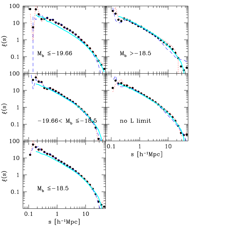
Figure 1: The redshift two-point correlation function of galaxies with different luminosity measured from the 2dFGRS catalog. The symbols with error bars are for the whole catalog, the dotted lines are for the southern subsample, and the dashed lines are for the northern subsample. The errors are estimated by the bootstrap resampling method. The luminosity ranges are indicated at each panel. The thick solid lines are the simulation predictions for the redhsift two-point correlation of dark matter in the WMAP concordance CDM model at redshift $z=0.13$.

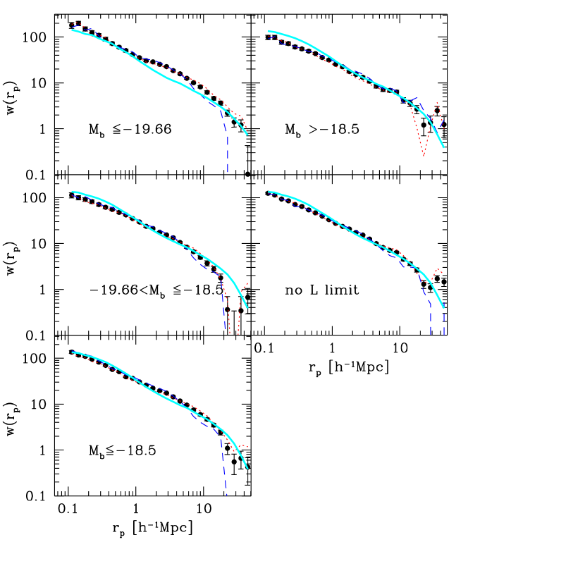
Figure 2: The projected two-point correlation function of galaxies with different luminosity measured from the 2dFGRS catalog. The symbols with error bars are for the whole catalog, the dotted lines are for the southern subsample, and the dashed lines are for the northern subsample. The errors are estimated by the bootstrap resampling method. The luminosity ranges are indicated at each panel. The thick solid lines are the simulation predictions for the projected two-point correlation of dark matter in the WMAP concordance CDM model at redshift $z=0.13$.

We have checked the random samples carefully by reproducing the angular distribution, mean redshift distribution, and especially the two-point statistics of clustering of the observed catalog. It is known that the two-point correlation function measured from galaxy catalogs on large scale is sensitive to the details of corrections for the above selection effects. We have estimated the redshift and projected correlation functions by the same method as in JMB98 for the Las Campanas Redshift Survey. The two-point correlation functions are shown in Figure 1 and Figure 2, and can be compared with the results of the 2dFGRS team for the clustering of galaxies (e.g. Hawkins et al., 2002; Norberg et al., 2002a). In addition to the broad agreement with their results, even the subtle difference between the north and south caps (the clustering on large scales is slightly larger in the southern cap than in the northern cap), and the luminosity dependence of the clustering, is well reproduced in our analysis.

We did not take into account in our analysis the fiber collision effect that two galaxies closer than $\sim 30$ arcsec cannot be assigned fibers simultaneously in one spectroscopic observation. Thus one of them will not have a redshift observation if no re-observation is arranged. This effect reduces the real space (or projected) two-point correlation function at small separations. With LCRS, JMB98 estimated the effect to lead to a 15 percent reduction in the two-point correlation function at projected separations $100\,h^{-1}{\rm{kpc}}$ and to a less than 5 percent reduction at separations larger than $400\,h^{-1}{\rm{kpc}}$. This effect is smaller (10 percent reduction at separations $100\,h^{-1}{\rm{kpc}}$) in the 2dFGRS (Hawkins et al., 2002), because the limiting fiber separation is slightly smaller (30 arc sec in the 2dFGRS vs 55 arcsec in the LCRS), and one field may be observed more than once in the 2dFGRS observation strategy. JB98 have examined the fiber collision effect on their measurement of the three-point correlation function of the LCRS. They found that the effect reduces the real space (projected) three-point correlation function at small separation, but changes little the normalized three-point correlations functions $Q$ that we will measure in this paper, because the effects on the two-point CF and three-point CF are canceled out when $Q$ is measured. Since the effect is slightly smaller in 2dFGRS in terms of the two-point clustering, we believe that only a negligible effect on our measurement of the normalized three-point correlations would result.

3 Statistical methods

We measure the three-point correlation functions for the galaxies in the 2dFGRS following the method of JB98. By definition, the joint probability $dP_{123}$ of finding one object simultaneously in each of the three volume elements $d{\mathbf{r}}_{1}$, $d{\mathbf{r}}_{2}$ and $d{\mathbf{r}}_{3}$ at positions ${\mathbf{r}}_{1}$, ${\mathbf{r}}_{2}$ and ${\mathbf{r}}_{3}$ respectively, is as follows (P80):

$$dP_{123}={\bar{n}}({\mathbf{r}}_{1}){\bar{n}}({\mathbf{r}}_{2}){\bar{n}}({\mathbf{r}}_{3})\bigl{[}1+\xi(r_{12})+\xi(r_{23})+\xi(r_{31})+\zeta(r_{12},r_{23},r_{31})\bigr{]}d{\mathbf{r}}_{1}d{\mathbf{r}}_{2}d{\mathbf{r}}_{3}$$ (9)

where $r_{ij}=|{\mathbf{r}}_{i}-{\mathbf{r}}_{j}|$, ${\bar{n}}({\mathbf{r}}_{i})$ is the mean density of galaxies at ${\mathbf{r}}_{i}$, and $\zeta(r_{12},r_{23},r_{31})$ is the three-point correlation function. This definition can be applied straightforwardly to redshift surveys of galaxies to measure the 3PCF $\zeta(s_{12},s_{23},s_{31})$ of galaxies in redshift space (at this point we neglect the anisotropy induced by the redshift distortion which will be considered later). Here and below we use $\mathbf{r}$ to denote the real space and $\mathbf{s}$ the redshift space.

The 3PCF of galaxies can be measured from the counts of different triplets (P80). Four types of distinct triplets with triangles in the range ($s_{12}\pm 1/2\Delta s_{12}$, $s_{23}\pm 1/2\Delta s_{23}$, and $s_{31}\pm 1/2\Delta s_{31}$) are counted: the count $DDD(s_{12},s_{23},s_{31})$ of triplets formed by three galaxies; the count $DDR(s_{12},s_{23},s_{31})$ of triplets formed by two galaxies and one random point; the count $DRR(s_{12},s_{23},s_{31})$ of triplets formed by one galaxy and two random points; the count $RRR(s_{12},s_{23},s_{31})$ of triplets formed by three random points. The random sample of points is generated in the way described in the previous section. Following the definition [eq(9)], we shall use the following estimator

$$\zeta(s_{12},s_{23},s_{31}) = {27RRR^{2}(s_{12},s_{23},s_{31})\times DDD(s_{12},s_{23},s_{31})\over DRR^{3}(s_{12},s_{23},s_{31})}$$ (10)

$$-{9RRR(s_{12},s_{23},s_{31})\times DDR(s_{12},s_{23},s_{31})\over DRR^{2}(s_{12},s_{23},s_{31})}+2$$

to measure the 3PCF of the galaxies in redshift space. The above formula is slightly different from the estimator used by Groth & Peebles (1977). Here we have extended the argument of Hamilton (1993) for the 2PCF to the case of the 3PCF. The coefficients $27$ and $9$ are due to the fact that only distinct triplets are counted in this paper. Since the early work of Peebles and coworkers (P80) indicates that the 3PCF of galaxies is approximately hierarchical, it is convenient to express the 3PCF in a normalized form $Q_{red}(s_{12},s_{23},s_{31})$:

$$Q_{red}(s_{12},s_{23},s_{31})={\zeta(s_{12},s_{23},s_{31})\over\xi(s_{12})\xi(s_{23})+\xi(s_{23})\xi(s_{31})+\xi(s_{31})\xi(s_{12})}\,.$$ (11)

It is also convenient to use the variables introduced by Peebles (P80) to describe the shape of the triangles formed by the galaxy triplets. For a triangle with the three sides $s_{12}\leq s_{23}\leq s_{31}$, $s$, $u$, and $v$ are defined as:

$$s=s_{12},\hskip 28.45274ptu={{s_{23}}\over{s_{\rm 12}}},\hskip 28.45274ptv={{s_{31}-s_{23}}\over{s_{12}}}\,.$$ (12)

Clearly, $u$ and $v$ characterize the shape and $s$ the size of a triangle. We take equal logarithmic bins for $s$ and $u$ with the bin intervals $\Delta\log s=\Delta\log u=0.2$, and equal linear bins for $v$ with $\Delta v=0.2$. For our analysis, we take the following ranges for $s$, $u$ and $v$: $0.63\leq s\leq 10\,h^{-1}{\rm{Mpc}}$ ($6$ bins); $1\leq u\leq 4$ (3 bins); and $0\leq v\leq 1$ (5 bins).

As in JB98, we have generalized the ordinary linked-list technique of $\rm P^{3}M$ simulations (Hockney & Eastwood, 1981) to spherical coordinates to count the triplets. The linked-list cells are specified by the spherical coordinates, i.e. the right ascension $\alpha$, the declination $\delta$ and the distance $s$. With this short-range searching technique, we can avoid the triplets out of the range specified thus making counting triplets very efficient. Because the triplet count $RRR$ is proportional to the third power of the number density of random points, the count within a fixed range of triangles would vary significantly among different luminosity subsamples if the number of random points is fixed, since the volumes covered by different subsamples are very different. We want to have random samples such that the random counts and the cross counts are as big as possible in order to suppress any uncertainty from the limited number of random points. Therefore, since the CPU time for counting triplets is approximately proportional to the total count of triplets in our linked list method, we choose the number of random points as large as possible for the computations of $RRR$, $DRR$, or $RDD$ under the condition that each computation is finished in $\mathrel{\raise 1.16pt\hbox{$<$}\kern-7.0pt\lower 3.06pt\hbox{{$\scriptstyle\sim$}}}24$ CPU hours on a Pentium IV 2.2 Ghz PC. The number of random points ranges from $40,000$ (for Sample IV) to $120,000$ (for Sample I) when computing $RRR$, and increases to $600,000$ (for Sample I) when computing $RDD$. The counts $RRR$ for small triangles ($s<1\,h^{-1}{\rm{Mpc}}$) could still be small, and therefore we have recalculated the counts $RRR$ for $s_{31}\leq 4\,h^{-1}{\rm{Mpc}}$ by generating a random sample 10 times larger, so as to ensure that the counts $RRR$ are at least $\sim 300$ for the triangle configurations of interest. We scaled these counts properly when we determined the three-point correlation function through equation (10). The uncertainty caused by the number of random points is negligible compared to the sampling errors of the observational sample.

The 3PCF in redshift space $Q_{red}(s,u,v)$ depends both on the real space distribution of galaxies and on their peculiar motions. Although this information contained in $Q_{red}(s,u,v)$ is also useful for the study of the large scale structures (see §4), it is apparent that $Q_{red}(s,u,v)$ is different from $Q(r,u,v)$ in real space. In analogy with the analysis for the two-point correlation function, we have determined the projected three-point correlation function $\Pi(r_{p12},r_{p23},r_{p31})$. We define the redshift space three-point correlation function $\zeta_{z}(r_{p12},r_{p23},r_{p31},\pi_{12},\pi_{13})$ through:

$$dP^{z}_{123} = {\bar{n}}({\mathbf{s}}_{1}){\bar{n}}({\mathbf{s}}_{2}){\bar{n}}({\mathbf{s}}_{3})\bigl{[}1+\xi_{z}(r_{p12},\pi_{12})+\xi_{z}(r_{p23},\pi_{23})+\xi_{z}(r_{p31},\pi_{31})$$ (13)

$$+\zeta_{z}(r_{p12},r_{p23},r_{p31},\pi_{12},\pi_{13})\bigr{]}d{\mathbf{s}}_{1}d{\mathbf{s}}_{2}d{\mathbf{s}}_{3}$$

where $dP^{z}_{123}$ is the joint probability of finding one object simultaneously in each of the three volume elements $d{\mathbf{s}}_{1}$, $d{\mathbf{s}}_{2}$ and $d{\mathbf{s}}_{3}$ at positions ${\mathbf{s}}_{1}$, ${\mathbf{s}}_{2}$ and ${\mathbf{s}}_{3}$; $\xi_{z}(r_{p},\pi)$ is the redshift space two-point correlation function; $r_{pij}$ and $\pi_{ij}$ are the separations of objects $i$ and $j$ perpendicular to and along the line-of-sight respectively. The projected 3PCF $\Pi(r_{p12},r_{p23},r_{p31})$ is then defined as:

$$\Pi(r_{p12},r_{p23},r_{p31})=\int\zeta_{z}(r_{p12},r_{p23},r_{p31},\pi_{12},\pi_{13})d\pi_{12}d\pi_{23}$$ (14)

Because the total amount of triplets along the line-of-sight is not distorted by the peculiar motions, the projected 3PCF $\Pi(r_{p12},r_{p23},r_{p31})$ is related to the 3PCF in real space $\zeta(r_{12},r_{23},r_{31})$ :

$$\Pi(r_{p12},r_{p23},r_{p31})=\int\zeta(\sqrt{r_{p12}^{2}+y_{12}^{2}},\sqrt{r_{p23}^{2}+y_{23}^{2}},\sqrt{r_{p31}^{2}+(y_{12}+y_{23})^{2}})dy_{12}dy_{23}\,.$$ (15)

Similarly as for $\zeta(s_{12},s_{23},s_{31})$, We measure $\zeta_{z}(r_{p12},r_{p23},r_{p31},\pi_{12},\pi_{13})$ similarly to $\zeta(s_{12},s_{23},s_{31})$ by counting the numbers of triplets $DDD(r_{p12},r_{p23},r_{p31},\pi_{12},\pi_{13})$, $DRR(r_{p12},r_{p23},r_{p31},\pi_{12},\pi_{13})$, $RDD(r_{p12},r_{p23},r_{p31},\pi_{12},\pi_{13})$ and $RRR(r_{p12},r_{p23},r_{p31},\pi_{12},\pi_{13})$ formed by galaxies and/or random points with the projected separations $r_{p12}$, $r_{p23}$, and $r_{p31}$ and radial separations $\pi_{12}$ and $\pi_{23}$. We will use $r_{p}$, $u$ and $v$:

$$r_{p}=r_{p12},\hskip 28.45274ptu={{r_{p23}}\over{r_{p12}}},\hskip 28.45274ptv={{r_{p31}-r_{p23}}\over{r_{p12}}}\,.$$ (16)

to quantify a triangle with $r_{p12}\leq r_{p23}\leq r_{p31}$ on the plane perpendicular to the line of sight. Equal logarithmic bins of intervals $\Delta\log r_{p}=\Delta\log u=0.2$ are taken for $r_{p}$ and $u$, and equal linear bins of $\Delta v=0.2$ for $v$. The same ranges of $u$ and $v$ are used as for $\zeta(s,u,v)$, but $r_{p}$ is from $0.128\,h^{-1}{\rm{Mpc}}$ to $4\,h^{-1}{\rm{Mpc}}$ (7 bins). The radial separations $\pi_{12}$ and $\pi_{23}$ are from $-25\,h^{-1}{\rm{Mpc}}$ to $25\,h^{-1}{\rm{Mpc}}$ with a bin size of $1\,h^{-1}{\rm{Mpc}}$. The projected 3PCF is estimated by summing up $\zeta_{z}(r_{p},u,v,\pi^{i}_{12},\pi^{j}_{23})$ at different radial bins ($\pi^{i}_{12},\pi^{j}_{23}$):

$$\Pi(r_{p},u,v)=\sum_{i,j}\zeta_{z}(r_{p},u,v,\pi^{i}_{12},\pi^{j}_{23})\Delta\pi^{i}_{12}\Delta\pi^{j}_{23}$$ (17)

and normalized as

$$Q_{proj}(r_{p},u,v)={\Pi(r_{p},u,v)\over w(r_{p12})w(r_{p23})+w(r_{p23})w(r_{p31})+w(r_{p31})w(r_{p12})}\,.$$ (18)

where $w(r_{p})$ is the projected two-point correlation function (Davis & Peebles, 1983, JMB98)

$$w(r_{p})=\sum_{i}\xi_{z}(r_{p},\pi^{i})\Delta\pi^{i}$$ (19)

An interesting property of the projected 3PCF is that if the three-point correlation function is of the hierarchical form, the normalized function $Q_{proj}(r_{p},u,v)$ is not only a constant but also equal to $Q$. Therefore the measurement of $Q_{proj}(r_{p},u,v)$ can be used to test the hierarchical form which was proposed mainly based on the analysis of angular catalogs.

Jing & Börner (1998) have used N-body simulations to test the statistical methods for the LCRS, and found that the results obtained are unbiased. Since the 2dFGRS is constructed in a similar way to the LCRS and the survey area is larger, the above methods should also yield unbiased results for the 2dFGRS.

The error bars of $Q$ are estimated by the bootstrap method (Barrow, Bhavsar, & Sonoda, 1984; Mo, Jing, & Börner, 1992). We have also used the mock samples of dark matter particles in §4 to estimate the error bars. We find that the error bars from these two methods agree within a factor of 2. Here we adopt the bootstrap error for the measurement of $Q$, since we do not input a luminosity-dependent bias for mock samples.

As in the analysis of the 2PCF, the estimates of the 3PCF given by Eq.(10) are correlated on different scales. This point should be taken into account when the measured 3PCF is compared with model predictions. Recently, there are new techniques developed to tackle this important issue in the context of the 2PCF or the power spectrum, e.g., Tegmark, Hamilton, & Xu (2002) and Matsubara & Szalay (2002) using the Karhunen-Loève eigenmode analysis, and Fang & Feng (2000) and Zhan, Jamkhedkar, & Fang (2001) using the wavelet analysis. It remains an important task to study if these methods can be extended to obtain a decorrelated 3PCF.

4 Results of the 2dFGRS Analysis

4.1 The 3PCF of the 2dFGRS catalog, and the luminosity dependence

We present the results of the 3PCF in redshift space $Q_{red}(s,u,v)$ and of the projected 3PCF $Q_{proj}(r_{p},u,v)$ in Figures 3 to 12 for the 2dFGRS survey. The errors of the Q-values are estimated by the bootstrap resampling method. The large number of galaxies in the 2dFGRS survey allows us to look for a possible luminosity dependence of $Q_{red}(s,u,v)$ and $Q_{proj}(r_{p},u,v)$. We have selected five galaxy samples according to luminosity, listed in Table 1. The samples are not completely independent with significant overlaps between some of the samples.

For $Q_{red}(s,u,v)$ the results are shown in Figures 3 to 7. As we can see , the 3PCF in redshift space is not changing very much with $s$ or $u$, it increases somewhat with $v$ for fixed $s$ and $u$. For small $v$ $Q_{red}(s,u,v)$ is approximately constant at a value of $\sim 0.6$, but it increases up to $\sim 1$, when $v\sim 1$.

For the bright galaxies we find that $Q_{red}(s,u,v)$ decreases somewhat with $s$, from $0.9$ at $s=0.82\,h^{-1}{\rm{Mpc}}$ to $0.4$ at $s=5.15\,h^{-1}{\rm{Mpc}}$. Changes with $s$ are slightly reduced for the samples including fainter galaxies. For the faintest sample (IV), at small $s$ and $v$ $Q_{red}(s,u,v)$ is about $1.1$, and it decreases to $\sim 0.7$ at $s=3.25\,h^{-1}{\rm{Mpc}}$.

We find that $Q_{red}(s,u,v)$ is slightly larger for the fainter samples, though the dependence on luminosity is rather weak. In fact, if the errors are taken into account, this luminosity dependence is not statistically significant. We also note that there is always some difference between the north strip, the south strip, and the whole sample, but generally within the $1\sigma$ error bars. This implies that the bootstrap error used in this sample is a good indicator for the error estimate. The results for the north and the south samples are in good agreement for the galaxies brighter than $M_{b}-5\log h\leq-18.5$. For the faint sample with $M_{b}-5\log h>-18.5$, however, there is a significant difference between the north and south subsamples. The main reason is that this sample covers only a small cosmic volume, so the sample-to-sample difference (the cosmic variance) can be large. In fact, even the 2PCFs of these subsamples are dramatically different (see Figure 1). Considering the fact that the bootstrap error is not sufficient to fully account for the cosmic variance, one should remain cautious about the result of the faintest sample (IV). Nonetheless, from Figures 3 to 7 we conclude that there is at best a slight dependence on luminosity in the sense that the amplitude $Q_{red}(s,u,v)$ tends to be smaller for brighter galaxies.

The projected 3PCF in comparison shows a behavior which is somewhat different. In the bright galaxy sample (Figure 8) $Q_{proj}(r_{p},u,v)$ is about 0.7 at $r_{p}=0.2\,h^{-1}{\rm{Mpc}}$, and it reaches down to $Q_{proj}(r_{p},u,v)\simeq 0.5$ at $r_{p}=3.25\,h^{-1}{\rm{Mpc}}$ for small $v$, so the dependences on $r_{p}$ is quite mild. There is, however, a small but significant increase with $v$. Fainter galaxies show a similar weak dependence on $r_{p}$ and $v$ (Figures 9 and 11). But comparing different samples, we find a trend that brighter galaxies have lower values of $Q_{proj}(r_{p},u,v)$. The $Q_{proj}(r_{p},u,v)$ of the fainter samples (II and IV) is about 50% higher than that of the brightest sample of $M_{b}-5\log h<-19.6$. We will discuss the implications for the bias parameters in §4.3.

The figures show that while the values of $Q_{proj}(r_{p},u,v)$ are similar for the north and south subsamples, the value for the total sample is larger than that of either subsample. This looks a bit surprising at first glance. But considering that the 2PCF of the north sample is almost 1.5 times larger than that of the south sample on $\,h^{-1}{\rm{Mpc}}$ scales, it is not difficult to explain the behavior of $Q_{proj}(r_{p},u,v)$ of the total sample and the two subsamples. As an idealized example, we assume that the two subsamples are well separated and have the same sample size, the same $Q_{proj}(r_{p},u,v)$, but the 2PCF of one sample is 1.5 times larger than that of the other. This example is quite close to the real situation of the faintest sample. It is not difficult to prove that the $Q_{proj}(r_{p},u,v)$ of the total sample is 1.4 times that of the subsamples. With this example, it is easy to see that the amplitude $Q_{proj}(r_{p},u,v)$ of the total sample is larger than that of the subsamples for $r_{p}=1.29\sim 3.25\,h^{-1}{\rm{Mpc}}$ for the faintest galaxies. This unusual behavior again can be attributed to the fact that this sample surveys only a small volume of sky, so the cosmic variance is large.

4.2 Comparison with the results from the LCRS

In Figure 13 we compare the normalized 3PCF in redshift space $Q_{red}(s,u,v)$ of the 2dFGRS and Las Campanas surveys. The data of the LCRS are taken from JB98 for galaxies with luminosities in the R-band $M_{R}-5\log h\leq-18.5$. From the 2dFGRS we simply take our result for the galaxies with $M_{b}-5\log h\leq-18.5$, although we are aware of the fact that the galaxies are selected in different wavebands in the two surveys. There are subtle differences in the results which we attribute to this choice of the observational bands, because $Q$ depends on luminosity weakly for $M>M^{*}$. For small values of $s\sim 1\,h^{-1}{\rm{Mpc}}$, the 2dF catalog gives a slightly higher amplitude than the LCRS galaxies. This could reflect the fact that the real space 2PCF of the LCRS galaxies is higher than that of the APM galaxies on small scales, as JMB98 pointed out. Nevertheless, the $Q_{red}(s,u,v)$ values agree very well between the two samples, especially on larger scales. The 2dF sample gives rise to a much smaller error, because of its large sample size.

To compare the projected amplitudes $Q_{proj}(r_{p},u,v)$, we display this quantity for the two catalogs in Figure 14. Again the agreement is quite satisfactory, especially when we take the larger error bars for the LCRS result into consideration. However, the systematic decrease with $r_{p}$ that can be read off for the mean values of $Q_{proj}(r_{p},u,v)$ for the LCRS data, is not present for the 2dFGRS. This is probably caused by the fact that the sky area of the LCRS is much smaller than the 2dFGRS survey, so the mean value of the LCRS is systematically underestimated. The 2dFGRS data also imply that the real space 3PCF of galaxies on the small scales explored here, does not deviate significantly from the hierarchical form (P80), and that the fitting formula given in JB98 for the projected $Q_{proj}(r_{p},u,v)$ needs to be revised.

In conclusion, our 2dFGRS results of $Q$, both in redshift space and in projected space, are in good agreement with the results obtained by JB98 for the LCRS.

4.3 Comparison with the dark matter distribution in the running power Cold Dark Matter model

In this section, we compare the observational results with model predictions. Currently, the parameters of the Cold Dark Matter (CDM) model have been determined pretty accurately by a combination of data from WMAP, 2dFGRS, Lyman-$\alpha$ absorption systems, and complementarily by many other observations (Spergel et al., 2003). We choose the running power CDM model of Spergel et al. for comparison with our statistical results, for this model matches most available observations: The universe is flat with a density parameter $\Omega_{0}=0.26$ and a cosmological constant $\lambda_{0}=0.74$. The Hubble constant is $71\,{\rm{km\,s^{-1}}}{\rm Mpc}^{-1}$ and the baryonic density parameter $\Omega_{0,b}=0.045$. The primordial density power spectrum deviates slightly from the Zhe’dovich spectrum as $P(k)\propto(k{\rm Mpc}/0.05)^{n(k)}$ with $n(k)=0.93-0.0165\ln(k{\rm Mpc}/0.05)$. Although there is no consensus about the necessity of introducing the running power index $n(k)$ (e.g. Seljak, McDonald, & Makarov, 2003; Tegmark et al., 2003), we choose this model as a reasonable approximation to the real situation.

Because the three-point correlation functions which we have measured, are in the non-linear and quasilinear regimes, we use a N-body simulation to make model predictions. The simulation has $512^{3}$ particles in a cubic box of $1024\,h^{-1}{\rm{Mpc}}$, and is generated with our $\rm P^{3}M$ code (see Jing & Suto, 2002, for the code). To include the effect of baryonic matter oscillations on large scale structures, the fitting formula of Eisenstein & Hu (1999) for the transfer function is used to generate the initial condition. Since the median redshift of the 2dFGRS is $\sim 0.13$, we choose the simulation output at this redshift. We note that the three-point correlation is quite sensitive to the presence of very massive clusters, therefore a large simulation box like the one used here is necessary. With a small box of $\mathrel{\raise 1.16pt\hbox{$<$}\kern-7.0pt\lower 3.06pt\hbox{{$\scriptstyle\sim$}}}100\,h^{-1}{\rm{Mpc}}$ the three-point correlation function may be underestimated severely.

Generally speaking, galaxies are biased tracers of the underlying matter distribution in the Universe. A luminosity dependence of the bias (Norberg et al., 2002a) means that faint and bright galaxies trace the matter distribution differently. It has become popular in recent years to account for the bias of certain types of galaxies phenomenologically with the so-called halo occupation model (e.g., Jing, Mo, & Börner, 1998; Seljak, 2000; Peacock & Smith, 2000; Sheth, Hui, Diaferio, & Scoccimarro, 2001; Berlind & Weinberg, 2002; Cooray & Sheth, 2002; Zehavi et al., 2003; Yang, Mo, & van den Bosch, 2003a, for an updated account of this model). The three-point correlation function of galaxies can also be modeled within this framework (Jing & Börner, 1998; Berlind & Weinberg, 2002; Ma & Fry, 2000; Takada & Jain, 2003, for a detailed account of this modeling), though it seems difficult to account for the two-point and three-point correlation functions in the LCRS simultaneously with simple power-law occupation models (Jing & Börner, 1998). Our accurate measurement of the 3PCF for the 2dFGRS and its luminosity-dependence will certainly provide an even more stringent constraint on the halo occupation models. It remains to be seen, if the sophisticated model of Yang et al. (2003a,b) can explain the results obtained in this paper. We want to investigate this issue in a subsequent paper, and here we only compare with one model prediction for the dark matter, in order to set a baseline quantifying the difference in the normalized three point correlation function between real galaxies and dark matter for the concordance CDM model.

The comparison between the 2dFGRS results and the model predictions is displayed in Figures 15 to 18. Here we consider only two luminosity subsamples. First, we find that the qualitative features, such as the dependence on $v$ for fixed $s$ or $r_{p}$, and $u$, the decrease of $Q$ with increasing values of $s$ or $r_{p}$ are reproduced quite well by the DM simulations. For the luminous sample (Sample I), the $Q$ values of the data set are generally lower than the dark matter model predictions, up to a factor $1.5\sim 2$. For the less luminous sample (Sample II), the observed $Q$ values also are smaller than those of the dark matter on small scales, but the observed values and the model predictions agree at the values $s\approx 8\,h^{-1}{\rm{Mpc}}$ and $r_{p}=3.25\,h^{-1}{\rm{Mpc}}$. Because the largest scales probed here are expected to be linear or quasilinear scales, we expect the linear bias model (eq.2) to hold on these scales. Our result therefore tells us that on linear scales, the galaxies of $-19.66<M_{J}-5\log h\leq-18.5$ are approximately an unbiased tracer, but the brightest galaxies of $M_{J}-5\log h\leq-19.66$ have a bias factor $\sim 1.5$.

Because the 2PCF of the galaxies of Sample II matches well the 2PCF of the dark matter in the concordance WMAP model, and our 3PCF results show that the galaxies of Sample II are unbiased on large, linear scales, we find support for the density fluctuation normalization $\sigma_{8}=0.84$ obtained by (Spergel et al., 2003). On the other hand, our result shows that the three-point correlations $Q$ of galaxies are lower on non-linear scales than the prediction of the WMAP concordance model. Physical models, e.g. the halo occupation number model (e.g. Yang, Mo, & van den Bosch, 2003a) or the semi-analytical models of galaxy formation (e.g., Kauffmann, Nusser, & Steinmetz, 1997) are needed to interpret the observed small scale non-linear bias. We will pursue this in a future paper. The three-point correlation amplitudes of Sample III and Sample V are very close to that of Sample II. The $Q$ of these samples gradually conforms to the model prediction of the concordance model on quasilinear scales $r\sim 5\,h^{-1}{\rm{Mpc}}$. Our results are therefore consistent with the analysis of Verde et al. who showed that the 2dFGRS galaxies (without a luminosity classification) are an unbiased tracer of the underlying matter on scales $5$ to $30\,h^{-1}{\rm{Mpc}}$.

5 Conclusion

In a detailed analysis of the 3PCF for the 2dFGRS survey we have accurately measured the 3PCF for galaxies of different luminosity. The 3PCF amplitudes ($Q_{red}(s,u,v)$ or $Q_{proj}(r_{p},u,v)$) of galaxies generally decrease with the increase of the triangle size and increase with the increase of $v$, qualitatively in agreement with the predictions for the dark matter clustering in popular hierarchical CDM models. Some dependence on luminosity is found, but not a strong effect, except for the brightest galaxy sample which seems to have lower amplitudes of up to $50\%$. Comparing with the previous study on the LCRS galaxies (JB98), we find good agreement between the two studies, though the results from the 2dFGRS are more accurate, since the 2dFGRS survey is much larger than the LCRS survey. The amplitudes in redshift space $Q_{red}(s,u,v)$ are very similar, but the projected ones $Q_{proj}(r_{p},u,v)$ show some difference. It seems that the projected 3PCF from the LCRS is systematically underestimated for $r_{p}$ in the range of a few $\,h^{-1}{\rm{Mpc}}$, because of the thin slice geometry of that survey. The dependence of $Q_{proj}(r_{p},u,v)$ on $r_{p}$ is much weaker in the 2dFGRS survey than in the LCRS survey.

Comparing the measured 3PCF amplitudes ($Q_{red}(s,u,v)$ or $Q_{proj}(r_{p},u,v)$) to the prediction of a WMAP concordance model, we find that the measured values are consistently lower than the predicted ones for dark matter. As in the case of the LCRS about one-half of the predicted $Q$ value provides a good description of $Q_{proj}(r_{p},u,v)$ for the 2dFGRS data. As in JB98 for the LCRS data, we may state that the best fit DM model gives higher values for the 3PCF than observed. This indicates that the simple DM models must be refined, either by using more sophisticated bias models, or a more sophisticated combination of model parameters.

The division of galaxies into luminosity classes reveals that the brightest galaxies are biased even on large scales, while the galaxies of sample II show a nonlinear bias on small scale, but appear unbiased on linear scales.

Figure 3: The normalized 3PCF in redshift space $Q_{red}(s,u,v)$ of galaxies with luminosity $M_{b}-5\log h\leq-19.66$ in the 2dFGRS survey. The results for the south strip, the north strip, and the whole sample are plotted with thick lines, thin lines, and symbols respectively. Different lines and symbols are used for triangle configurations of different $u$ as indicated on the figure. The errors are estimated by the bootstrap resampling method. For clarity, the error bars are plotted for the whole sample and $u=2$ only, but those for the other two values of $u$ are very similar, and for north or south strips are about $1.4$ times larger.

Figure 4: The normalized 3PCF in redshift space $Q_{red}(s,u,v)$ of galaxies with luminosity $-19.66<M_{b}-5\log h\leq-18.5$ in the 2dFGRS survey. The notations are the same as Fig.3.

Figure 5: The normalized 3PCF in redshift space $Q_{red}(s,u,v)$ of galaxies with luminosity $M_{b}-5\log h\leq-18.5$ in the 2dFGRS survey. The notations are the same as Fig.3.

Figure 6: The normalized 3PCF in redshift space $Q_{red}(s,u,v)$ of galaxies with luminosity $M_{b}-5\log h>-18.5$ in the 2dFGRS survey. The notations are the same as Fig.3.

Figure 7: The normalized 3PCF in redshift space $Q_{red}(s,u,v)$ of all galaxies in the 2dFGRS survey (without luminosity selection). The notations are the same as Fig.3.

Figure 8: The normalized projected 3PCF $Q_{proj}(r_{p},u,v)$ of galaxies with luminosity $M_{b}-5\log h\leq-19.66$ in the 2dFGRS survey. The results for the south strip, the north strip, and the whole sample are plotted with thick lines, thin lines, and symbols respectively. Different lines and symbols are used for triangle configurations of different $u$ as indicated on the figure. The errors are estimated by the bootstrap resampling method. For clarity, the error bars are plotted for the whole sample and $u=2$ only, but those for the other two values of $u$ are very similar, and for the north or south strip are about $1.4$ times larger.

Figure 9: The normalized projected 3PCF $Q_{proj}(r_{p},u,v)$ of galaxies with luminosity $-19.66<M_{b}-5\log h\leq-18.5$ in the 2dFGRS survey. The notations are the same as Fig.8.

Figure 10: The normalized projected 3PCF $Q_{proj}(r_{p},u,v)$ of galaxies with luminosity $M_{b}-5\log h\leq-18.5$ in the 2dFGRS survey. The notations are the same as Fig.8.

Figure 11: The normalized projected 3PCF $Q_{proj}(r_{p},u,v)$ of galaxies with luminosity $M_{b}-5\log h>-18.5$ in the 2dFGRS survey. The notations are the same as Fig.8.

Figure 12: The normalized projected 3PCF $Q_{proj}(r_{p},u,v)$ of all galaxies in the 2dFGRS survey (without luminosity selection). The notations are the same as Fig.8.

Figure 13: Comparison of the normalized 3PCFs in redshift space $Q_{red}(s,u,v)$ measured from the 2dFGRS and from the Las Campanas Redshift Survey (LCRS). The data of the LCRS are taken from Jing & Börner (1998) for galaxies with luminosity in the R-band $M_{R}-5\log h\leq-18.5$. For comparison, we simply take our result in the 2dFGRS survey of galaxies with $M_{b}-5\log h\leq-18.5$, despite the fact that galaxies are selected in different wavebands in the two surveys. The results of the LCRS are plotted in solid symbols, and those of the 2dFGRS are in open symbols. The errors are estimated by the bootstrap resampling method, and are plotted for $u=2$ only. For clarity, the symbols are shifted by $+0.05$ for the LCRS and by $-0.05$ for 2dFGRS along the horizontal axis.

Figure 14: Comparison of the normalized projected 3PCFs $Q_{proj}(r_{p},u,v)$ measured from the 2dFGRS and from the Las Campanas Redshift Survey (LCRS). The data of the LCRS are taken from Jing & Börner (1998) for galaxies with luminosity in the R-band $M_{R}-5\log h\leq-18.5$. For comparison, we simply take our result in the 2dFGRS survey of $M_{b}-5\log h\leq-18.5$, despite the fact that the galaxies are selected in different wavebands in the two surveys. The results of the LCRS are plotted in solid symbols, and those of the 2dFGRS are in open symbols. The errors are estimated by the bootstrap resampling method, and are plotted for $u=2$ only. For clarity, the symbols are shifted by $+0.05$ for the LCRS and by $-0.05$ for 2dFGRS along the horizontal axis.

Figure 15: Comparison of the normalized 3PCF of galaxies in redshift space $Q_{red}(s,u,v)$ with the function predicted in the WMAP running power CDM model. The observed data (sysmbols) are from the 2dFGRS survey for $M_{b}-5\log h\leq-19.66$, and the model prediction is for dark matter (lines). The errors are estimated by the bootstrap resampling method, and are plotted for $u=2$ only.

Figure 16: Comparison of the normalized 3PCF of galaxies in redshift space $Q_{red}(s,u,v)$ with the function predicted in the WMAP running power CDM model. The observed data (sysmbols) are from the 2dFGRS survey for $-19.66<M_{b}-5\log h\leq-18.5$, and the model prediction is for dark matter (lines). The errors are estimated by the bootstrap resampling method, and are plotted for $u=2$ only.

Figure 17: Comparison of the normalized projected 3PCF of galaxies $Q_{proj}(r_{p},u,v)$ with the function predicted in the WMAP running power CDM model. The observed data (sysmbols) are from the 2dFGRS survey for $M_{b}-5\log h\leq-19.66$, and the model prediction is for dark matter (lines). The errors are estimated by the bootstrap resampling method, and are plotted for $u=2$ only.

Figure 18: Comparison of the normalized projected 3PCF of galaxies $Q_{proj}(r_{p},u,v)$ with the function predicted in the WMAP running power CDM model. The observed data (sysmbols) are from the 2dFGRS survey for $-19.66<M_{b}-5\log h\leq-18.5$, and the model prediction is for dark matter (lines). The errors are estimated by the bootstrap resampling method, and are plotted for $u=2$ only.

Table 1: Samples selected according to luminosity

Sample	$M_{b}-5\log h$	South	North	Total
I	$M_{b}-5\log h\leq-19.66$	16702	11761	28463
II	$-19.66<M_{b}-5\log h\leq-18.5$	14247	11798	26045
III	$M_{b}-5\log h\leq-18.5$	30949	23559	54508
IV	$M_{b}-5\log h>-18.5$	7930	6572	14502
V	no limit	39208	30447	69655

References

- Bahcall & Comerford (2002) Bahcall N.A., Comerford J.M., 2002, ApJ, 565, L5
- Barriga & Gaztañaga (2002) Barriga, J. & Gaztañaga, E. 2002, MNRAS, 333, 443
- Barrow, Bhavsar, & Sonoda (1984) Barrow, J. D., Bhavsar, S. P., & Sonoda, D. H. 1984, MNRAS, 210, 19P
- Bartelmann & Schneider (2001) Bartelmann, M., & Schneider, P. 2001, Physics Reports, 340, 291
- Bean et al. (1983) Bean A.J., Efstathiou G., Ellis R.S., Peterson B.A., Shanks T., 1983, MNRAS, 205, 605
- Benson et al. (2000) Benson A. J., Baugh C. M., Cole S., Frenk C. S., Lacey C. G., 2000, MNRAS, 316, 107
- Berlind & Weinberg (2002) Berlind, A. A. & Weinberg, D. H. 2002, ApJ, 575, 587
- Bernardeau, Colombi, Gaztañaga, & Scoccimarro (2002) Bernardeau, F., Colombi, S., Gaztañaga, E., & Scoccimarro, R. 2002, Phys. Rep., 367, 1
- Börner, Deng, Xia, & Zhou (1991) Börner, G., Deng, Z.-G., Xia, X.-Y., & Zhou, Y.-Y. 1991, Ap&SS, 180, 47
- Buchalter & Kamionkowski (1999) Buchalter, A. & Kamionkowski, M. 1999, ApJ, 521, 1
- Catelan et al. (1998) Catelan. P., Lucchin, F., Matarrese, S., Porciani, C. 1997, MNRAS (submitted); astro-ph/9708067
- Colless et al. (2001) Colless, M. et al. 2001, MNRAS, 328, 1039
- Cooray & Sheth (2002) Cooray, A. & Sheth, R. 2002, Phys. Rep., 372, 1
- Davis et al. (1985) Davis, M., Efstathiou, G., Frenk, C. S., & White, S. D. M. 1985, ApJ, 292, 371
- Davis & Peebles (1983) Davis M., Peebles P.J.E., 1983, ApJ, 267, 465
- Efstathiou & Jedrzejewski (1984) Efstathiou, G., & Jedrzejewski, R.I. 1984, Adv. Space Res., 3, 379
- Eisenstein & Hu (1999) Eisenstein, D. J. & Hu, W. 1999, ApJ, 511, 5
- Fang & Feng (2000) Fang, L. & Feng, L. 2000, ApJ, 539, 5
- Frieman & Gaztañaga (1999) Frieman, J. A. & Gaztañaga, E. 1999, ApJ, 521, L83
- Fry (1984) Fry J.N., 1984, ApJ, 279, 499
- Gaztañaga & Frieman (1994) Gaztañaga E., Frieman J.A., 1994, ApJ, 437, L13
- Groth & Peebles (1977) Groth, E.J., & Peebles, P.J.E. 1977, ApJ, 217, 385
- Hale-Sutton et al. (1989) Hale-Sutton, D., Fong, R., Metcalfe, N., Shanks, T. 1989, MN, 237, 569
- Hamilton (1993) Hamilton A.J.S., 1993, ApJ, 417, 19
- Hamilton & Tegmark (2002) Hamilton, A. J. S. & Tegmark, M. 2002, MNRAS, 330, 506
- Hawkins et al. (2002) Hawkins et al. 2002, astro-ph/0212375
- Hockney & Eastwood (1981) Hockney R.W., Eastwood J.W., 1981, Computer simulations using particles. McGraw-Hill Inc., New York
- Jing & Börner (1997) Jing, Y.P., Börner, G. 1997, A&A, 318, 667
- Jing & Börner (1998) Jing, Y. P. & Börner, G. 1998, ApJ, 503, 37
- Jing, Mo, & Börner (1991) Jing, Y.P., Mo, H.J., & Börner, G. 1991, A&A, 252, 449
- Jing, Mo, & Börner (1998) Jing, Y. P., Mo, H. J., & Börner, G. 1998, ApJ, 494, 1
- Jing & Suto (2002) Jing, Y. P. & Suto, Y. 2002, ApJ, 574, 538
- Kauffmann, Colberg, Diaferio, & White (1999) Kauffmann, G., Colberg, J. M., Diaferio, A., & White, S. D. M. 1999, MNRAS, 303, 188
- Kauffmann, Nusser, & Steinmetz (1997) Kauffmann, G., Nusser, A., & Steinmetz, M. 1997, MNRAS, 286, 795
- Lahav, et al., (2002) Lahav O., et al., 2002, MNRAS, 333, 961
- Lauberts (1982) Lauberts, A. 1982, The ESO-Uppsala Survey of the ESO(B) Atlas, European Southern Observatory
- Loveday, Maddox, Efstathiou, & Peterson (1995) Loveday, J., Maddox, S. J., Efstathiou, G., & Peterson, B. A. 1995, ApJ, 442, 457
- Ma & Fry (2000) Ma, C. & Fry, J. N. 2000, ApJ, 531, L87
- Matarrese, Verde, & Heavens (1997) Matarrese, S., Verde, L., Heavens, A. 1997, MNRAS (in press); astro-ph/9706059
- Matsubara (1994) Matsubara T. 1994, ApJ, 424, 30
- Matsubara & Szalay (2002) Matsubara, T. & Szalay, A. S. 2002, ApJ, 574, 1
- Mo, Jing, & Börner (1992) Mo, H.J., Jing, Y.P., & Börner, G. 1992, ApJ, 392, 452
- Mo, Jing, & White (1997) Mo, H.J., Jing, Y.P., White, S.D.M., 1997, MNRAS, 284, 189
- Norberg et al. (2002a) Norberg, P. et al. 2002a, MNRAS, 332, 827
- Norberg et al. (2002b) Norberg, P. et al. 2002b, MNRAS, 336, 907
- Peacock & Smith (2000) Peacock, J. A. & Smith, R. E. 2000, MNRAS, 318, 1144
- Peebles (1980) Peebles P.J.E., 1980, The Large-Scale Structure of the Universe, Princeton University Press, Princeton
- Peebles (1981) Peebles, P.J.E. 1981, in Annals New York Academy of Science, 157
- Pen et al. (2003) Pen, U.-L. et al. 2003, astroph/0304512
- Scoccimarro, et al. (1998) Scoccimarro, R., Colombi, S., Fry, J. N., Frieman, J. A., Hivon, E., Melott, A. 1998, ApJ, 496, 586