A 3D Monte Carlo Photoionization Code for Modeling Diffuse Ionized Gas

Abstract

We have developed a three dimensional Monte Carlo photoionization code tailored for the study of Galactic H ii regions and the percolation of ionizing photons in diffuse ionized gas. We describe the code, our calculation of photoionization, heating & cooling, and the approximations we have employed for the low density H ii regions we wish to study. Our code gives results in agreement with the Lexington H ii region benchmarks. We show an example of a 2D shadowed region and point out the very significant effect that diffuse radiation produced by recombinations of helium has on the temperature within the shadow.

1 Introduction

A major characteristic of the interstellar medium (ISM) is that it is clumpy, with filamentary structure over scales ranging from hundreds of parsecs through sub-AU cloudlets. The spatial density of electrons is approximately a power law over an astonishing 12 orders of magnitude (, Armstrong et al.1995), from $\sim$300 pc to $<$0.1 AU in the ISM. The magnetic field of the Galaxy varies in a similar fashion on scales from 0.01 to 100 pc. Molecular clouds show a fractal (scale-free) spatial variation of the intensity of CO (e.g., Falgarone, Phillips, & Walker 1991) and neutral H (Stanimirović & Lazarian, 2001). Sub-parsec variations are shown by the variation of ionic column densities along different ISM sightlines towards individual stars in close binaries (Lauroesch, Meyer, & Blades, 2000). Large area velocity resolved surveys of the molecular (e.g., Simon et al. 2001), neutral (e.g., Hartmann & Burton 1999), and ionized (Reynolds, Haffner, & Madsen, 2002) gas now allow us to probe the geometry, kinematics, ionization, and temperature structure of the ISM.

Our development of Monte Carlo radiation transfer techniques to study photon scattering, ionization, and radiative equilibrium dust temperatures in complex geometries is motivated by these and the many other observations that clearly require three dimensional modeling analyses. In this paper we describe improvements and extensions to our Monte Carlo photoionization code (Wood & Loeb, 2000) that will enable us to model the 3D temperature, ionization structure, emission line images, and spectra of low density H ii regions and the Diffuse Ionized Gas (DIG), often called “the warm ionized medium” or “Reynolds layer”. This diffuse ionized gas has a complicated structure and surely requires three-dimensional modeling, both as regards the sources of its ionization and the transfer of the ionizing radiation. How can Lyman continuum photons from O and B stars percolate from their midplane origins to ionize the high latitude gas? A non-uniform ISM is required that provides low density paths for ionizing photons to reach the halo. Using a “Strömgren volume” ionization technique and a statistical approach to clumping, Miller & Cox (1993) showed that O and B stars can ionize the DIG (see also Dove & Shull 1994; Dove, Shull, & Ferrara 2000). Using Monte Carlo simulations for hydrogen ionization, Ciardi et al. (2002) have investigated ionization structures in a fractal ISM as proposed by Elmegreen (1997). In Elmegreen’s picture, the observed H$\alpha$ emission may arise from the ionized surfaces of fractal clouds. This suggestion clearly needs to be investigated with 3D radiation transfer techniques.

Other features of the DIG that may require 3D analyses are the temperature structure and relative ionization structure of He and H. The temperature of the DIG, as determined from line intensity ratios (e.g., Reynolds, Haffner, & Tufte 1999), appears to require additional heating over and above that provided by photoionization heating (Mathis, 2000). Among the possible heating mechanisms, dissipation of energy in a turbulent medium has been proposed (Minter & Spangler, 1996), definitely 3D! Another question is, can clumping/shadowing explain the apparent lack of He⁰ in H⁺ regions (Reynolds & Tufte, 1995)? In this scenario, direct stellar photons are prevented from ionizing He in shadow regions behind dense clumps, but diffuse ionizing photons from H and He recombinations can percolate into the shadow regions and ionize H, but not He.

Our work on the analysis of scattered light in fractal reflection nebulae (Mathis, Whitney, & Wood, 2002) highlighted the crucial role of geometry when trying to determine dust properties from scattered light observations. Much of what we know about abundances of elements comes from analysis of spectra utilizing one-dimensional photoionization techniques (see e.g. Stasińska 2002). Over the last decade several three dimensional photoionization codes have been developed. The code presented by Baessgen, Diesch, & Grewing (1990) uses the “on the spot” approximation for the diffuse radiation field, while that of Gruenwald, Viegas, & Broguiere (1997) employs an adaptive mesh grid and an iterative procedure to determine the contribution of the diffuse radiation field. Monte Carlo techniques naturally include diffuse radiation within three dimensional systems and Monte Carlo photoionization codes have been described by Ercolano et al. (2003) for the three-dimensional case and Och, Lucy, & Rosa (1998) for the one-dimensional case.

We have extended our basic hydrogen-only Monte Carlo photoionization code (Wood & Loeb, 2000) to treat the photoionization, heating, & cooling for the complex geometry expected in low density H ii regions and the diffuse ISM. Our code is similar to those described by Och, Lucy, & Rosa (1998) and Ercolano et al. (2003), but calculates the rates of photoionization and heating “on the fly”, rather than calculating the mean intensity of the radiation field (see also Lucy 1999). It also treats reprocessing of radiation in a different manner to that described by Och, Lucy, & Rosa (1998), using “photon packets” rather than “energy packets.”

In §2 we describe our assumptions and approximations to model the DIG. §3 describes the Monte Carlo technique, our method of discretizing the radiation field into “photon packets” rather than “energy packets,” and how we determine the diffuse radiation field using ratios of recombination rates. §4, §5, & §6 deal with our photoionization and heating/cooling algorithms, §7 presents the atomic data used in our code, and §8 compares our code with standard H II region benchmarks and gives an example of a 2D calculation.

2 Approximations for the DIG

We make the following assumptions and approximations for the opacity, heating and cooling.

• We consider only radiation energetic enough to ionize H ($h\nu\geq$13.6 eV). Photons of lower energies are ignored until we calculate the emergent intensities of certain spectral features after the simulation is completed.

• All ions are in the ground state when they absorb radiation or recombine with an electron. This is the standard “nebular approximation.” The low-lying levels giving rise to fine structure lines might be an exception. Radiative transfer in these lines would require consideration of the populations of the levels involved in their production. We assume that the fine structure lines are optically thin.

• No H-ionizing photons are produced by recombinations to excited levels of H or He. This is because $kT_{e}\ll\chi$(H⁰) = 13.6 eV, the ionization potential of H.

• There is no collisional ionization or de-excitation. In effect, this limits the densities we can study to be less than a few $\times 10^{3}$ cm^-3, which is generally above that encountered in the Diffuse Ionized Gas and typical H II regions, but within the typical range of planetary nebulae.

• There is no He⁺² because the stellar radiation field has negligible luminosity above 54.4 eV, consistent with observations of almost all H ii regions.

• The opacity is due to continuous opacity from neutral H and He; we ignore contributions from other ions because of their low abundances. At present we ignore all other opacity sources (e.g., dust, UV metal line blanketing, etc.) except photoionization from oxygen.

• Photoionization and heating by the He I Lyman $\alpha$ line is included in an “on-the-spot” approximation (see §4.1 for a discussion of the physics).

• We keep track of the abundances of the stages of ionization of H, He, C, N, O, Ne, and S that have their ionization potentials $\geq\,\chi({\rm H}^{0})$ and $\leq\,\chi(\rm{He}^{+})$ = 54.4 eV. These are H⁰, He⁰, C⁺ – C⁺³, N⁰ – N⁺³, O⁰ – O⁺², Ne⁰ – Ne⁺³, and S⁺ – S⁺³. These chemical elements are chosen because some of their ions are important for the heating and cooling rates. It is straightforward to include other elements, but they do not appreciably affect the H and He ionization structure or contribute to the heating or cooling. We assume that there is no S⁰ because its ionization potential is 10.36 eV, so it is ionized by the ambient stellar radiation fields softer than $h\nu$ = 13.6 eV (see Savage & Sembach 1996 for observations).

• Heating arises solely from the photoionization of H and He. Cooling is from recombinations of H and He, free-free emission, and collisionally excited line radiation from N, O, Ne, S (see below).

• We ignore dynamics, turbulence, and the effects of shocks and ionization fronts.

It is straightforward to include more ions and the effects of dust opacity. The assumption of no opacity from heavy elements may also be easily relaxed.

3 Monte Carlo Photoionization

We want to determine the time-independent ionization and temperature structure of a nebula with an assumed fixed density distribution. We do this by Monte Carlo radiative transfer followed by iterations to find the ionization structure that determines the opacity.

Within each iteration we consider packets of ionizing photons emitted from the exciting star(s) of the nebula. We choose the frequency from the probability distribution of the photon emission from the sources. We follow each stellar photon packet through the density grid until it is absorbed and causes photoionization. The subsequent recombination often results in the production of another ionizing photon packet, thereby forming the diffuse radiation field. The frequency of the new packet is sampled from various atomic probability distributions. We first determine if the packet was absorbed by H⁰ or He⁰, and then determine the frequency of the re-emitted packet (see below). We continue the Monte Carlo random walk of absorption/re-emission events until the packet is re-emitted with $h\nu<13.6$ eV, at which time we terminate it.

3.1 Photon Packets versus Energy Packets

Our approach differs somewhat from previous Monte Carlo simulations (Och, Lucy, & Rosa 1998; Lucy 1999; Bjorkman & Wood 2001; Ercolano et al. 2003) that followed the energy of a packet, rather than its number of photons. Considering energy is natural for investigating problems of radiative equilibrium (e.g., scattering and thermal emission by dust, or stellar atmospheres), since the energy that is absorbed is thermally re-emitted with exactly the same energy but with a source function, $S_{\nu}$, given by Kirchhoff’s Law ($S_{\nu}\equiv j_{\nu}/k_{\nu}=B_{\nu}(T)$, where $j_{\nu}$ is the emissivity and $k_{\nu}$ the absorption coefficient). Kirchhoff’s Law is applicable only when the populations of atomic levels are in Local Thermodynamic Equilibrium and does not apply to nebulae. The number of photons associated with an energy packet varies with its frequency, so it is not as straightforward to apply atomic probabilities in following the fate of an energy packet. The energy of an energy packet is given by $\epsilon=L\,\Delta t/N$ and is kept constant for radiative equilibrium codes, where $L$ is the stellar luminosity, $\Delta t$ is the time covered by the simulation, and $N$ is the number of packets used in the simulation. The energies of our packets are $\epsilon=Q\,h\nu\,\Delta t/N$, where $Q$ is the ionizing photon luminosity (units s^-1). The energy is not kept constant as the packet changes frequency, but keeps its number of photons constant (see also Lucy 2003).

Since our initial goal is to determine the 3D ionization and temperature structure, we do not follow the non-ionizing diffuse photons: they are emitted with $h\nu<13.6$ eV and will escape from the nebula, so we terminate the ionizing photon and start a new one from the star. We thus save memory by not having to form probability distribution functions in each cell for finding the frequency of non-ionizing photons. Rather, we determine a converged ionization and temperature structure and then employ a second code to integrate numerically through our resulting emissivity grid to form the emergent spectrum and images in various spectral lines.

Current desktop machines using 1Gb RAM can handle grids of around $128^{3}$ cells for our code. The iterative photoionization and heating calculation (described in §4 and 5) updates the temperature and ionic fractions of all species we are tracking in each cell throughout the grid. At the end of each iteration we have a new ionization structure and opacity grid for the next iteration.

3.2 Emission Direction and Frequency

In Monte Carlo techniques we must decide on the outcome of events that depend on some physical variable, say $x$ (e.g., the frequency $\nu$), with a given probability, $P(x)$. The important quantity is the cumulative distribution function, $C(x)$, given by

$$C(x)={{\int_{x_{-}}^{x}\,P(x^{\prime})\,\rm dx^{\prime}}\over\int_{x_{-}}^{x_{+}}\,P(x^{\prime})\,\rm dx^{\prime}}\;,$$

where $x_{-}$ is the minimum value of $x$ and $x_{+}$ the maximum. We find a randomly selected value of $x$ by casting a random number, $\xi$, in the range [0,1] and inverting the relation $\xi=C(x)$.

We assume the density structure of our nebular simulation, possibly quite complex as appropriate to the ISM. We begin the Monte Carlo radiation transfer by emitting photon packets from the exciting star(s) with an initial guess for the ionization structure. The initial guess for the ionization structure does not affect the final converged solution, but it does affect the number of iterations required for convergence. For isotropic emission, the random directions are

$$\cos\theta=2\xi-1$$ (1)

$$\phi=2\pi\xi\;,$$ (2)

where $\theta$ and $\phi$ are the usual spherical polar coordinates. The direction cosines for the initial photon trajectories are then given by

$$n_{x}=\sin\theta\cos\phi$$ (3)

$$n_{y}=\sin\theta\sin\phi$$ (4)

$$n_{z}=\cos\phi\;.$$ (5)

The photon frequency must be sampled to reproduce the ionizing spectrum of the source, $L(\nu)$, which may be a blackbody or model atmosphere. We pre-tabulate the cumulative photon distribution function,

$$C(\nu_{i})={{\int_{\nu_{H^{0}}}^{\nu_{i}}L(\nu)/h\nu\,{\rm d}\nu}\over{\int_{\nu_{H^{0}}}^{\infty}L(\nu)/h\nu\,{\rm d}\nu}}\;.$$ (6)

A random frequency is chosen by solving for $\nu$ in $\xi=C(\nu)$ by interpolating in the pre-tabulated cumulative distribution function $C(\nu_{i})$. From $\nu$ we calculate the photoionization cross sections $a_{\nu}({\rm H}^{0})$ and $a_{\nu}({\rm He}^{0})$ from analytic formulae. The optical depth, $\tau_{\nu}$, along a path length $S$ is

$$\tau_{\nu}=\int_{0}^{S}[n({\rm H}^{0})a_{\nu}({\rm H}^{0})+n({\rm He}^{0})a_{\nu}({\rm He}^{0})]\,{\rm d}s\;.$$ (7)

where $n({\rm H}^{0})$ and $n({\rm He}^{0})$ vary from cell to cell. We generate a random optical depth by $\tau=-\log\xi$ and integrate through the opacity grid until the distance $S$ has been reached. If the distance $S$ lies outside the simulation grid the photon has exited our simulation and we start another packet from the star.

3.3 The Diffuse Radiation Field

On finding the position associated with the randomly chosen optical depth, we decide if the photon packet is absorbed by H⁰ or He⁰. The packet is absorbed by H⁰ if $\xi\leq n({\rm H}^{0})a_{\nu}({\rm H}^{0})/[n({\rm H}^{0})a_{\nu}({\rm H}^{0})+n({\rm He}^{0})a_{\nu}({\rm He}^{0})]$, and by He⁰ otherwise. If absorbed by H⁰, it will be re-emitted either as a Lyman continuum photon (and subsequently tracked with the Monte Carlo technique) or terminated. If absorbed by He⁰ there are several energy channels into which it can be re-emitted as described below. Once a photon packet has been absorbed we re-emit it with a frequency chosen using the following algorithm.

3.3.1 H I Emission

The probability that the photon is emitted in the hydrogen Lyman continuum is

$$P({\rm H~{}I~{}Ly~{}c})={{\alpha_{1}({\rm H}^{0},T_{e})}\over{\alpha_{A}({\rm H}^{0}\;,T_{e})}}\;,$$ (8)

where $\alpha_{1}$ is the recombination coefficient to the ground level and $\alpha_{A}$ the coefficient to all levels, including $n$ = 1. The packet emerges in the Lyman continuum if $\xi\leq P({\rm Ly~{}c})$. If the packet is chosen to be re-emitted in the Lyman continuum, we sample its frequency using the $C(\nu)$ derived from the Saha-Milne emissivity:

$${C}_{\rm{Lyc}}(\nu,T_{e})=\int_{\nu_{0}}^{\nu}(j_{\nu}/h\nu)\,{\rm d}\nu/\int_{\nu_{0}}^{\infty}(j_{\nu}/h\nu)\,{\rm d}\nu\;;$$ (9)

$$j_{\nu}={{2h\nu^{3}}\over{c^{2}}}\,\left({h^{2}}\over{2\pi\,m_{e}\,k\,T_{e}}\right)^{3/2}$$ (10)

$$\times\;a_{\nu}({\rm H^{0}}){\rm e}^{-h(\nu-\nu_{0})/kT_{e}}n({\rm H}^{+})n_{\rm e}\;.$$ (11)

We pre-tabulate $C_{\rm{Lyc}}(\nu,\,T_{e})$ and from $\xi=C(\nu,T_{e})$ we determine $\nu$ from $\xi$ by interpolating in the table. The packet is now re-emitted with a direction chosen from an isotropic distribution (Eqs. 1 and 2).

At the start of each iteration we form a 3D grid that contains $P({\rm H~{}I~{}Ly~{}c})$ and use this grid to decide the fate of photon packets absorbed by H⁰. Similar grids are formed for the He emission probabilities as described in the next section. These probability grids are updated after each iteration since the recombination rates are temperature dependent.

3.3.2 He I Emission

An absorption by He is followed by recombination and possibly by radiative cascades into either the metastable levels $2^{1}S$ or $2^{3}S$, to $2^{1}P$ (the upper level of Lyman $\alpha$), or to the ground level $1^{1}S$. The probabilities for emission in these four channels are as follows:

1. He I Lyman continuum ($h\nu>24.6$ eV) is analogous to that given for H in §3.3.1.

2. The probability of emission as a 19.8 eV photon packet from the transition $2^{3}S\rightarrow 1^{1}S$ is

   $$P(19.8\,{\rm eV})={{\alpha_{2^{3}S}^{\rm eff}({\rm He}^{0},T_{e})}\over{\alpha_{A}({\rm He}^{0},T_{e})}}\;.$$ (12)

   The effective recombination rate takes into account all means of populating the given level, both direct recombination and via cascades from higher levels, from which low energy photons are emitted.

3. The probability of emission from the He I two-photon continuum from $2^{1}S$ is

   $$P({\rm He~{}I}\,2q)={{\alpha_{2^{1}S}^{\rm eff}({\rm He}^{0},T_{e})}\over{\alpha_{A}({\rm He}^{0},T_{e})}}\;.$$ (13)

   Note that $\alpha_{2^{1}S}^{\rm eff}({\rm He}^{0},T_{e})$ does not include de-excitations from $2^{1}P$, which will be discussed in §4.1

   A fraction 0.28 of the photons in this emission channel is able to ionize H⁰, so the number of photons emitted per decay is 2(0.28) = 0.56 photons. After determining that the packet is to be emitted in the 2-photon continuum, we see if $\xi\leq 0.56$. If so, we choose a frequency from a pre-tabulated $C(\nu)$ for two-photon emission (Drake, Victor, & Dalgarno 1969, Table II).

4. The probability of emission as a He I Lyman $\alpha$ photon ($h\nu=21.2$ eV) is

   $$P({\rm He\,I\,Ly\,\alpha})={{\alpha_{2^{1}P}^{\rm eff}({\rm He}^{0},T_{e})}\over{\alpha_{A}({\rm He}^{0},T_{e})}}\;.$$ (14)

   Och, Lucy, & Rosa (1998) and Ercolano et al. (2003) followed energy packets of several of the He I Lyman lines, assuming that the various He Lyman lines are absorbed only by the H⁰ continuous opacity, propagating through the grid and maintaining their identity without degrading into Lyman $\alpha$. We do not follow this prescription because resonance lines will be scattered many times without diffusing far in space. Following each scattering from $n^{1}P$ ($n\geq 2$), there is a finite probability of re-emission into a lower excited level rather than to 1${}^{1}S$. Subsequent emissions from that excited level cascade downwards and populate either $2^{1}S$ or $2^{1}P$. Conversion to $2^{1}S$ is followed by He I 2-photon continuum emission. We discuss our treatment of the $2^{1}P$ in §4.1.

To form the various probabilities, we use analytic fits to the temperature dependent recombination rates for H and He. These rates, along with all other atomic data, are presented in §7. Since there are only four He I levels with appreciable populations, we have

$$\alpha_{A}=\alpha_{1}+\alpha_{2^{1}S}^{\rm eff}+\alpha_{2^{1}P}^{\rm eff}+\alpha_{2^{3}S}^{\rm eff}\;.$$ (15)

We also assume that recombinations to triplets produce only the 19.8 eV 2${}^{3}S\rightarrow 1^{1}S$ transition. We do not follow $2^{3}P\rightarrow 1^{1}S$, as did Och, Lucy, & Rosa (1998), since at low densities 2${}^{3}P$ converts to 2${}^{3}S$ via 10830Å emission.

4 Photoionization

We must calculate the photoionization, heating, and cooling in order to update the ionic fractions and electron temperature after each iteration.

The basic photoionization equations, in the notation of Osterbrock (1989), are

$$n(X^{+i})\int_{\nu_{i}}^{\infty}{{4\pi J_{\nu}}\over{h\nu}}a_{\nu}(X^{+i}){\rm d}\nu=n(X^{+i+1})n_{\rm e}\alpha(X^{+i},T_{e}),$$ (16)

where $n(X^{+i})$ and $n(X^{+i+1})$ are the number densities (per cm³) of successive stages of ionization, $\nu_{i}$ is the threshold for photoionization from $X^{+i}$, $n_{\rm e}$ is the electron number density, and $\alpha(X^{+i},T_{e})$ is the recombination coefficient to all levels of $X^{+i}$. In our code the photon luminosity of the sources, $Q$, is divided into $N$ packets, so we calculate the integral on the left of eqn. (16) by

$$I^{P}_{X^{+i}}=\int_{\nu_{i}}^{\infty}{{4\pi J_{\nu}}\over{h\nu}}a_{\nu}(X^{+i}){\rm d}\nu={{Q}\over{N\,\Delta V}}\sum la_{\nu}(X^{+i})\;.$$ (17)

where the summation is over all path lengths through the volume $\Delta V$ for photons in the frequency range ($\nu,\nu+{\rm d}\nu$), and $l$ is the path length of each photon counted in the sum (Lucy 1999, 2003).

Thus, we do not explicitly calculate the mean intensity $J_{\nu}$ throughout the grid in order to compute the integral of $4\pi J_{\nu}a_{\nu}(X^{+i})/h\nu$ for each ion considered. To save $J_{\nu}$, we would need storage for each grid cell with as many frequencies as being considered.

We add the contribution of each ionizing photon packet, regardless of stellar or nebular origin, to the sum of $l\,a_{\nu}(X^{+i})$ maintained for each ion, within each cell in the grid. At the end of the iteration we have a 3D array for each ion that contains the integral $I^{P}_{X^{+i}}(x,y,z)$. The photoionization rate is then $n(X^{+i})\,I^{P}_{X^{+i}}$ within each cell. So long as the number of ions being tracked is less than the typical number of frequencies required for an accurate representation of the mean intensity, our technique will save significantly on memory storage. We use the above equations to solve the ionization balance of most ions that we follow. Exceptions to this are our treatment of He I Ly$\alpha$ photons that can ionize H⁰, and also charge exchange that couples the ionization of some ions to H and He.

We now outline our treatments of the ionization balance for these situations.

4.1 He I Lyman $\alpha$

We do not need to follow the diffusion of the He I Ly$\alpha$ resonance line ($2^{1}P\rightarrow 1^{1}S$) in space and frequency. The level $2^{1}P$ is depopulated either by emission of a He I Ly$\alpha$ photon ($2^{1}P\rightarrow 1^{1}S$) or a 2.06$\mu$m photon ($2^{1}P\rightarrow 2^{1}S$). Due to the large resonant line opacity, the He I Ly$\alpha$ will be scattered locally many times without traveling far. It will eventually be absorbed locally (“on the spot”) by H⁰ or else decay to $2^{1}S$.

Note that the “on the spot” approximation is used due to the large He I Ly$\alpha$ resonant opacity and not the H⁰ opacity.

What is $P({\rm H_{OTS}})$, the probability of the He I Ly$\alpha$ photon being absorbed by H⁰ as opposed to the transition $2^{1}P\rightarrow 2^{1}S$ occurring? The average number of resonant scatterings before decay to 2${}^{1}S$ is $A_{2^{1}P,1^{1}S}/A_{2^{1}P,2^{1}S}=914$ (Benjamin, Skillman, & Smits 1999). The mean free path between scatterings, $l_{\rm scat}$, is $[n({\rm He}^{0})\,a_{\nu}({\rm Ly}\alpha)]^{-1}$, where the line opacity is

$$a_{\nu}({\rm Ly}\alpha)=(\pi^{\frac{1}{2}}e^{2}/m_{e}c)\ f_{21}\,\exp[-(\Delta\nu/\Delta\nu_{D})^{2}]/\Delta\nu_{D}\ ,$$ (18)

where $f_{21}$, the oscillator strength of the transition, is 0.29. $\Delta\nu/\Delta\nu_{D}$ is the displacement of the frequency of the photon from the line center, in Doppler widths. This displacement is determined by the speed the atom had before recombination, and so has a Maxwellian probability distribution (if we neglect any non-thermal components in the local velocity distribution). The Maxwell-Boltzmann distribution can be written $f_{\rm MB}(v)\propto v^{2}\,\exp[-(v/v_{\rm th})^{2}]$ and $\Delta\nu/\Delta\nu_{D}=(v/v_{\rm th}$), with $v_{\rm th}=(2kT/M)^{1/2}$. We average over the line profile:

$$\langle\exp[-(\Delta\nu/\Delta\nu_{D})^{2}]\rangle$$ (19)

$$={{\int_{0}^{\infty}\exp[-(v/v_{\rm th})^{2}]\,v^{2}\exp[-(v/v_{\rm th})^{2}]\,{\rm d}v}\over{\int_{0}^{\infty}v^{2}\,\exp[-(v/v_{\rm th})^{2}]\,{\rm d}v}}$$

$$=2^{-3/2}\ .$$ (20)

The number of absorptions by H⁰ during the 914 scatterings is 914 $l_{\rm scat}\,n({\rm H}^{0})\,a_{\nu}({\rm H}^{0})$, with $a_{\nu}({\rm H}^{0})=1.9\times 10^{-18}$ cm². The probability of the photon being absorbed by H⁰ is

$$P({\rm H_{OTS}})={{n({\rm H}^{0})a_{\nu}({\rm H}^{0})}\over{[n({\rm H}^{0})\,a_{\nu}({\rm H}^{0})+n({\rm He}^{0})a_{\nu}({\rm He}^{0})/914]}}$$

$$=\left(1+0.77f({\rm He}^{0})/[f(\rm H^{0})(T/10^{4}\,\rm K)^{1/2}]\right)^{-1}\ ,$$ (21)

where $f({\rm He}^{0})$ and $f({\rm H}^{0})$ are the neutral fractions of He and H, respectively, and He/H = 0.1 in abundance has been assumed. The $f({\rm He}^{0})/f({\rm H}^{0})$ favors He, especially for softer exciting stars. For instance, the inner parts of the nebula surrounding a 40000 K black body favor He⁰ by a factor of $\sim$7, so 80% of transitions to 2${}^{1}P$ are converted to 2${}^{1}S$ rather than being absorbed by H⁰. For harder exciting spectra, the $f({\rm He}^{0})/f({\rm H}^{0})$ is $<$2, and a significant number of Ly$\alpha$ photons are absorbed by H⁰. Heating by Ly$\alpha$ is significantly greater than from 2-photon emission. However, the (2${}^{3}S\rightarrow 1^{1}S$) photons are far more important than any from the singlets as regards both ionization and heating.

In the “on-the-spot” treatment, local absorptions of Ly$\alpha$ are exactly balanced by local emissions. The rate of “on-the-spot” absorptions by H⁰ is $P({{\rm H}_{\rm OTS}})$ times the rate of recombinations into He${}^{0}(2^{1}P$), or $P({{\rm H}_{\rm OTS}})n({\rm He}^{+})\,n_{\rm e}\alpha^{\rm eff}({\rm He}^{0},2^{1}P)$. These absorptions by H⁰ are also given by $n({\rm H}^{0})\,a_{\nu}({\rm H}^{0})[4\pi\,J_{\nu}({\rm Ly}\alpha)/h\nu]$. By equating these rates, we obtain a modified ionization balance equation for H:

$$n({\rm H}^{0})\int_{\nu_{i}}^{\infty}(4\pi J_{\nu}/h\nu)a_{\nu}({\rm H}^{0}){\rm d}\nu=$$ (22)

$$n_{\rm e}[n({\rm H}^{+})\alpha({\rm H}^{0},T_{e})-P({{\rm H}_{\rm OTS}})n({\rm He}^{+})\alpha_{2^{1}P}^{\rm eff}]\;,$$ (23)

where the $J_{\nu}$ does not include He I Ly$\alpha$, which is contained in the final term on the right side of the equation.

4.2 Charge Exchange

The rate of exchange of an electron between an ion ($X^{+i}$) and H⁰ or He⁰ can be comparable to or exceed the radiative recombination rates. With our adopted charge exchange cross sections (Kingdon & Ferland, 1996), the rate of transitions into N⁺², O⁰, and O⁺ are seriously affected or dominated by exchange with H⁰. The opposite effect, in which charge exchange dominates the ionization of the lower stage, takes place for O⁰. A result is that in regions where O⁰ is important (i.e., H⁰ is appreciable), (O⁰/O${}^{+})\sim$ 9/8 (H⁰/H⁺) for all $T_{e}$ because the ionization potential of O⁰ is almost the same as for H⁰ (see Osterbrock 1989, p. 42 for a discussion.) For N⁰, charge exchange is not dominant but not negligible. We included the reactions in the rates for reactions resulting in N⁺ and O⁺ as well.

With charge exchange included, the (O⁰/O⁺) equation becomes

$$n({\rm O}^{0})\,[n_{e}\,\int 4\pi\,J_{\nu}/h\nu\,{\rm d}\nu+n({\rm H}^{+})\,C_{\rm exch}({\rm O}^{0},\,{\rm H}^{+})]=$$

$$n({\rm O}^{+})\,[n_{e}\,\alpha_{\rm rec}({\rm O}^{+})+n({\rm H}^{0})\,C_{\rm exch}({\rm O}^{+},\,{\rm H}^{0})]\;.$$

The situation regarding charge exchange with He⁰ is less clear because the cross section is very difficult to compute. We account for charge exchange with He⁰ for interactions resulting in N⁺, N⁺², and O⁺.

5 Heating & Cooling

The temperature is determined by finding the root of $G(T)={\cal L}(T)$, where $G$ and ${\cal L}$ are the heating and cooling rates due to the processes described below (see Chapter 3 of Osterbrock 1989).

5.1 Heating

We consider only heating by photoionization of H and He and calculate the heating rate in each grid cell in the same manner as we calculated the photoionization rate. For example, for photoionization of He the heating rate is

$$G({\rm He}^{0})=\int_{\nu_{{\rm He}^{0}}}^{\infty}{{4\pi J_{\nu}}\over{h\nu}}a_{\nu}({\rm He}^{0})\,h(\nu-\nu_{{\rm He}^{0}})\,{\rm d}\nu\;,$$ (24)

so we form integrals analogous to the photoionization rate

$$I^{H}_{\rm He}=\int_{\nu_{{\rm He}^{0}}}^{\infty}{{4\pi J_{\nu}}\over{h\nu}}a_{\nu}({\rm He}^{0})\,h(\nu-\nu_{{\rm He}^{0}})\,{\rm d}\nu=$$ (25)

$$[Q/(N\,\Delta V)]\sum la_{\nu}({\rm He}^{0})(h\nu-h\nu_{{\rm He}^{0}})\;.$$ (26)

As with photoionization, we assume “on-the-spot” heating by He I Ly$\alpha$ packets, so a term $P({\rm H_{OTS}})n({\rm He}^{+})n_{e}\alpha^{\rm eff}_{2^{1}P}({\rm Ly}\alpha)[h\nu({\rm Ly}\alpha)-\chi(\rm H^{0})]$ is added to the heating per volume of each cell.

5.2 Cooling from Recombination and Free-Free Radiation

Cooling rates as a function of temperature, $\cal L$, due to recombination of H⁺ and He⁺ are taken from Hummer (1994) and Hummer & Storey (1998). The cooling rate due to free-free radiation is given by Osterbrock (1989):

$${\cal L}_{\rm ff}=1.42\times 10^{-27}\,[n({\rm H}^{+})+n({\rm He}^{+})]\,n_{e}\,g_{\rm ff}\sqrt{T}_{e}\;,$$ (27)

where we use the Katz et al. (1996) fit to the free-free Gaunt factor data in Spitzer (1978)

$$g_{\rm ff}=1.1+0.34\,\exp{[-(5.5-\log T_{e})^{2}/3]}\;.$$ (28)

5.3 Other Cooling

We include collisional excitation of the lowest five levels of the ions of N⁰, N⁺,O⁰,O⁺,O⁺², Ne⁺², S⁺, and S⁺², and of 2 levels of N⁺² and Ne⁺, as in other photoionization codes (e.g., Ercolano et al. 2003). For this cooling by collisionally excited forbidden lines we use the Einstein A values and collision strengths from the compilation by Pradhan & Peng (1995) as updated on A. Pradhan’s webpage.

6 Some Code Details

After each iteration, we simultaneously solve for the ionization and temperature using the equations outlined above. The code will converge quickly if we have a good first guess of the ionization and temperature structure. However, for the 3D problems that we wish to address, such a guess will be very difficult to make. We therefore start the first iteration assuming that H and He are fully ionized, so all stellar photons exit the grid on the first iteration, but do contribute to the mean intensity counters. If we started with a neutral grid, photon packets could not diffuse far from their point of origin due to the large neutral opacity and convergence would be very slow, if at all.

As in Ercolano et al. (2003), we run several iterations with a small number of photon packets to get a rough idea of the ionization and temperature structure: $10^{6}$ packets for the first eight iterations, up to $10^{8}$ for higher iterations $\geq$20. Our models are well converged within 12 iterations; the higher iterations with large numbers of photon packets provide higher signal-to-noise for the ionization and temperature structure.

In 3D simulations, the diffuse field ionizes walls strongly inclined to the direction to the star. We find a good early approximation to the diffuse field by initially setting all cells to be fully ionized, thereby predicting the diffuse radiation field if the nebula were fully ionized. For the next iteration, if the stellar radiation cannot maintain a high degree of ionization the outer material becomes almost neutral, since the diffuse field is much weaker than the stellar field. The structure reaches a good approximation to the eventual diffuse field after about five iterations. If the shadowed regions were allowed to turn neutral before the diffuse field had converged, we would face the same convergence problem (with each new iteration ionizing a small zone of previously neutral material) described above.

We run our code on a single desktop machine within a reasonable CPU time (see Ercolano et al. 2003 for a discussion of code speed up via parallelization), running $\sim$1.0M photon packets per minute on a 2.4 GHz processor.

7 Atomic Data

We use standard references for the line and continuum emissivities (Brocklehurst 1972; Brown & Mathews 1970; Storey & Hummer 1995; Benjamin, Skillman, & Smits 1999). We take the photoionization cross section for H from the fitting formula of 1996. The recombination rate to all levels $\alpha_{A}({\rm H}^{0},T_{e})$ is given by the fitting formula in Verner & Ferland (1996). For the recombinations to the ground state, $1^{2}S$, we fitted the temperature dependent rates in Osterbrock (1989, Table 2.1), with

$$\alpha_{1}({\rm H}^{0},T_{e})=1.58\times 10^{-13}(T_{e}/10^{4}K)^{-0.53}\;.$$ (29)

For He we use the (1996) formula for the photoionization cross section. For the recombination rates we use the fitting formulae in Table 1 of Benjamin, Skillman, & Smits (1999) that give us the direct recombination rates to the ground level, $1^{1}S$, and the effective rate to $2^{3}S$. We calculated the effective rates to $2^{1}P$ and to $2^{1}S$, ignoring the $2^{1}P\rightarrow 2^{1}S$ transition because we separately consider its competition with absorption by H (see the discussion in §4.1). The rates to $2^{1}P$ and $2^{1}S$ were formed by adding the direct recombination rates (Benjamin, Skillman, & Smits (1999), Table 1), effective rates for $n>5$ (Table 3), and effective rates from all lines for $3\leq n\leq 5$ that connect to the appropriate lower level (Table 5). In summary,

$$\alpha_{1}({\rm He}^{0},T_{e})=1.54\times 10^{-13}(T_{e}/10^{4})^{-0.486}$$ (30)

$$\alpha_{2^{1}S}^{\rm eff}({\rm He}^{0},T_{e})=2.06\times 10^{-14}(T_{e}/10^{4})^{-0.676}$$ (31)

$$\alpha_{2^{1}P}^{\rm eff}({\rm He}^{0},T_{e})=4.17\times 10^{-14}(T_{e}/10^{4})^{-0.861}$$ (32)

$$\alpha_{2^{3}S}^{\rm eff}({\rm He}^{0},T_{e})=2.10\times 10^{-13}(T_{e}/10^{4})^{-0.778}\;,$$ (33)

thus enabling us to form the probabilities for reprocessing packets by He (§3.3.2).

The ionization cross section for the ions we use are taken from (1996) and the radiative recombination rates are from Verner & Ferland (1996). Also important in the recombination are dielectronic recombination rates, for which we use values determined by Nussbaumer & Storey (1983, 1984, 1987) for N, O, and Ne. The dielectronic recombination rates for sulphur have not been calculated, and we normally use those recommended by Ali et al. (1991) for the first four ionization stages of S: $3\times 10^{-13}$, $3\times 10^{-12}$, $1.5\times 10^{-11}$, and $2.5\times 10^{-1}$, which are the mean rates for the first four atoms/ions of C, N, and O as discussed by Ali et al. (1991). The charge exchange rates are taken from Kingdon & Ferland (1996) for reactions with H⁰ and from Arnaud & Rothenflug (1985) for those with He⁰.

8 Some Results and Benchmarks

8.1 Lexington H II Region Benchmarks

Any 3D photoionization code must reproduce two benchmark tests of blackbody exciting stars ionizing uniform spherical nebulae of a specified composition. The benchmarks have been discussed extensively in workshops (Ferland et al. 1995, Péquignot et al. 2001; see these for the details of the input parameters). Results of many codes are given in Table 1 (for a 40kK central star) and Table 2 ($T_{*}$ = 20kK). The authors of the other codes are given in the footnote to Table 1. The dielectronic recombination coefficients assumed for S are zero for S⁺² and those in Ali et al. (1991) for S⁺³ and S⁺⁴. We believe these were adopted by most of the models in each table. Some models in the benchmark took the optical depths of fine structure lines into account, but we did not. Our results are given in the last column in each table.

Figure 1 shows plots of ionization and temperature with radius for the $T_{\star}$ =40000 K benchmark and compares our results (crosses) with the Monte Carlo photoionization code mocassin (Ercolano et al., 2003) (squares) and the widely used code cloudy (Ferland, 1994) (lines). Figure  2 presents the same quantities for the $T_{\star}$ = 20000 K benchmark. In comparing with mocassin, we set up the density grids to have the same spatial resolution: our code used a grid of $65^{3}$ cells and mocassin, which utilizes the symmetry of the benchmark, performed the radiation transfer in an $33^{3}$ octant. For these simulations our code used $10^{8}$ photon packets and mocassin used $6.4\times 10^{7}$ energy packets in the final (20th) iteration, though both codes had essentially converged by iteration 14. Among the three codes, the ionization fractions are all in very good agreement. Because of our 65³ grid resolution, our code produces slightly more ionization at the outer edge. There is a larger spread in the predicted temperatures for the hot benchmark, with our code being slightly hotter in the inner portions of the nebula and mocassin being slightly cooler towards the edge of the nebula. The agreement for the cool benchmark temperatures is very good.

The large spread of some ionization fractions (e.g., O⁺²/O in Fig. 2) illustrates a property of Monte Carlo codes unless special steps are taken. The ionization potential of O⁺ is 35.1 eV; an ionizing photon is so rare that even with $10^{8}$ photon packets there is considerable statistical noise. If an accurate prediction of the (O⁺²/O) were one of our goals, we could have forced energetic stellar photons to be emitted and then correct the results by the known probabilities of the events we forced.

The cubic nature and limited spatial resolution of our grid makes the comparison problematic for one ion, O⁰, mainly found in the very outermost regions of the nebula. In these regions, (O⁰/O⁺) = 9/8 H⁰/H⁺ because of a resonant charge exchange between O⁺ and H⁰. There is a rather sharp peak in the temperature because of the hardening of stellar radiation caused by selective absorption within the nebula, and a steep temperature gradient because of the large opacity. With better spatial resolution, the volume occupied by one cell would contain regions of almost neutral hydrogen, so the temperature assigned to the whole cell, and the strength of [O I] $\lambda$6300, are of limited meaning. We present results from our cells with H⁰/H $\leq$ 0.25; the cells more neutral than this amount occur in the outer $<$1% of the radius ($r_{\rm outer}=1.454\times 10^{19}$ cm for the 40kK benchmark model, as opposed to 1.463$\times 10^{19}$ cm for the average radial distance). In real H ii regions, dynamical effects dominate in these outer regions, where ionized gas is flowing away from the ionization front. With 65 cells on a side and the star at the centre, each cell has a width of 3% of the radius. Thus, the region we disregard (with hydrogen being $\geq$25% neutral) is much less than the width of each cell.

We want to identify “extreme” predictions, defined by being outside of the range shown by the other models. One way of describing them (Péquignot et al., 2001) is the “isolation factor”, the ratio of our value to the next most extreme.

For the 40kK benchmark, our code provides three extreme values, two within 4% of the nearest value. Our [S III] $\lambda$9532+9069 prediction is 12.5% larger than that from the Rubin code (RR in the table). Rubin’s code (RR), mocassin (BE), and Harrington’s (PH) are the only ones that use detailed radiative transfer rather than an approximation such as “outward only.”

For the 20kK benchmark, the results are very similar. We are extreme in six quantities, by $<$5% in all but two. The worst are [O III] $\lambda$5949,5007 and (52$\mu$m + 88$\mu$m), (10% and 8% more than T. Kalman’s xstar). We did not account for optical thickness in these lines, so our high predictions are understandable. Also, for this cool model our photon statistics for O⁺² are problematic, as discussed above. Since 1D codes can provide excellent spatial resolution by inserting zones wherever there are steep gradients, especially at the outer edges where the temperature is changing rapidly, we feel that the benchmark results are satisfactory.

One simple check is available for the cool model. There are relatively few He-ionizing stellar photons, and it is simple to show that He absorptions strongly dominate H for He-ionizing photons. Each He ionization is followed by the emission of 0.96 H-ionizing photons (Osterbrock, 1989). Thus, the ratio of $\langle{\rm He}^{+}\rangle/\langle{\rm H}^{+}\rangle$ is the ratio of the He-ionizing to H-ionizing stellar luminosities, 0.49 for a $T$ = 20 kK blackbody. Our code predicts 0.47, suggesting that our relatively coarse cell size is satisfactory for predicting He⁺/H⁺ and other ionic abundances.

Figure 1: HII40 benchmark, showing our Monte Carlo results (crosses), mocassin (squares), and the cloudy model (solid line).

Figure 2: HII20 benchmark, showing our Monte Carlo results (crosses), mocassin (squares), and the cloudy model (solid line).

Table 1: Lexington H ii Region Benchmark Results: HII40^a

Line/H$\beta$	GF	HN	DP	TK	PH	RS	RR	BE	WME
${\rm H}\beta/10^{36}{\rm erg\,s}^{-1}$	2.06	2.02	2.02	2.10	2.05	2.07	2.05	2.02	2.01
He i 5876	0.119	0.112	0.113	0.116	0.118	0.116	-	0.114	0.114
C ii 2325+	0.157	0.141	0.139	0.110	0.166	0.096	0.178	0.148	0.172
C iii 1907+1909	0.071	0.076	0.069	0.091	0.060	0.066	0.074	0.041	0.078
N ii 122$\mu$m	0.027	0.037	0.034	-	0.032	0.035	0.030	0.036	0.031
N ii 6584+6548	0.669	0.817	0.725	0.69	0.736	0.723	0.807	0.852	0.742
N ii 5755	0.0050	0.0054	0.0050	-	0.0064	0.0050	0.0068	0.0061	0.0057
N iii 57.3$\mu$m	0.306	0.261	0.311	-	0.292	0.273	0.301	0.223	0.308
O i 6300+6363	0.0094	0.0086	0.0088	0.012	0.0059	0.0070	-	0.0065	0.011
O ii 7320+7330	0.029	0.030	0.031	0.023	0.032	0.024	0.036	0.025	0.033
O ii 3726+3729	1.94	2.17	2.12	1.6	2.19	1.88	2.26	1.92	2.23
O iii 52+88$\mu$m	2.35	2.10	2.26	2.17	2.34	2.29	2.34	2.28	2.42
O iii 5007+4959	2.21	2.38	2.20	3.27	1.93	2.17	2.08	1.64	2.34
O iii 4363	0.00235	0.0046	0.0041	0.0070	0.0032	0.0040	0.0035	0.0022	0.0044
Ne ii 12.8$\mu$m	0.177	0.195	0.192	-	0.181	0.217	0.196	0.212	0.192
Ne iii 15.5$\mu$m	0.294	0.264	0.270	0.35	0.429	0.350	0.417	0.267	0.263
Ne iii 3869+3968	0.084	0.087	0.071	0.092	0.087	0.083	0.086	0.053	0.063
S ii 6716+6731	0.137	0.166	0.153	0.315	0.155	0.133	0.130	0.141	0.18
S ii 4068+4076	0.0093	0.0090	0.0100	0.026	0.0070	0.005	0.0060	0.0060	0.0094
S iii 18.7$\mu$m	0.627	0.750	0.726	0.535	0.556	0.567	0.580	0.574	0.623
S iii 9532+9069	1.13	1.19	1.16	1.25	1.23	1.25	1.28	1.21	1.44
$10^{3}\times\Delta({\rm BC}\,3645)$/Å	4.88	-	4.95	-	5.00	5.70	-	5.47	4.96
$T_{\rm inner}$/K	7719	7668	7663	8318	7440	7644	7399	7370	7743
$<T[{\rm N}_{p}{\rm N}_{e}]>$/K	7940	7936	8082	8199	8030	8022	8060	7720	8183
$R_{\rm out}/10^{19}$cm	1.46	1.46	1.46	1.45	1.46	1.47	1.46	1.46	1.45
$<{\rm He}^{+}{\rm H}^{+}>$	0.787	0.727	0.754	0.77	0.764	0.804	0.829	0.715	0.771
aGF, Ferland’s cloudy; HN, H. Netzer’s ion; DP, D. Péquinot’s nebu; TK, T. Kallman’s xstar;
PH, J. P. Harrington’s code; RS, R. Sutherland’s mappings; RR, R. Rubin’s nebula;
BE, B. Ercolano’s mocassin; WME, this paper.

Table 2: Lexington H ii Region Benchmark Results: HII20

Line/H$\beta$	GF	HN	DP	TK	PH	RS	RR	BE	WME
${\rm H}\beta/10^{36}{\rm erg\,s}^{-1}$	4.85	4.85	4.83	4.90	4.93	5.04	4.89	4.97	4.87
He i 5876	0.0072	0.008	0.0073	0.008	0.0074	0.0110	-	0.0069	0.00684
C ii 2325+	0.054	0.047	0.046	0.040	0.060	0.038	0.063	0.042	0.053
N ii 122$\mu$m	0.068	-	0.072	0.007	0.072	0.071	0.071	0.071	0.067
N ii 6584+6548	0.745	0.786	0.785	0.925	0.843	0.803	0.915	0.846	0.778
N ii 5755	0.0028	0.0024	0.0023	0.0029	0.0033	0.0030	0.0033	0.0025	0.0025
N iii 57.3$\mu$m	0.0040	0.0030	0.0032	0.0047	0.0031	0.0020	0.0022	0.0019	0.0049
O i 6300+6363	0.0080	0.0060	0.0063	0.0059	0.0047	0.0050	-	0.0088	0.055
O ii 7320+7330	0.0087	0.0085	0.0089	0.0037	0.0103	0.0080	0.0100	0.0064	0.0089
O ii 3726+3729	1.01	1.13	1.10	1.04	1.22	1.08	1.17	0.909	1.12
O iii 52+88$\mu$m	0.0030	0.0026	0.0026	0.0040	0.0037	0.0020	0.0017	0.0022	0.0044
O iii 5007+4959	0.0021	0.0016	0.0015	0.0024	0.0014	0.0010	0.0010	0.0011	0.0026
Ne ii 12.8$\mu$m	0.264	0.267	0.276	0.27	0.271	0.286	0.290	0.295	0.289
S ii 6716+6731	0.499	0.473	0.459	1.02	0.555	0.435	0.492	0.486	0.521
S ii 4068+4076	0.022	0.017	0.020	0.052	0.017	0.012	0.015	0.013	0.017
S iii 18.7$\mu$m	0.445	0.460	0.441	0.34	0.365	0.398	0.374	0.371	0.381
S iii 9532+9069	0.501	0.480	0.465	0.56	0.549	0.604	0.551	0.526	0.602
$10^{3}\times\Delta({\rm BC}\,3645)$/Å	5.54	-	5.62	-	5.57	5.50	-	6.18	5.52
$T_{\rm inner}$/K	7224	6815	6789	6607	6742	6900	6708	6562	6852
$<T[{\rm N}_{p}{\rm N}_{e}]>$/K	6680	6650	6626	6662	6749	6663	6679	6402	6692
$R_{\rm out}/10^{18}$cm	8.89	8.88	8.88	8.7	8.95	9.01	8.92	8.89	8.73
$<{\rm He}^{+}{\rm H}^{+}>$	0.048	0.051	0.049	0.048	0.044	0.077	0.034	0.041	0.047

8.2 Ionization in a Shadow Region

The structure of the shadow zone behind a small high-density clump of gas, such as those found in the planetary nebula NGC 7293, is of direct astrophysical interest. There have been several treatments of such a shadowed zone. Approximate static models have also been considered by Van Blerkom & Arny (1972) and Mathis (1976). An analytical treatment is given by Cantó et. al. (1998), who considered dynamical evolution of the shadowed region and its ionization and temperature structure. These assume that the radiation field incident upon the shadow is the diffuse field within the H ii region, estimated by assuming that the nebula is thick to its own diffuse radiation and that there is no diffuse radiation produced by He.

We tested the influence of He upon the ionization and temperature of a shadowed zone by comparing two models, one with the benchmark composition and one with the same H and heavy elements but no helium. Both used the geometry similar to that in Cantó et. al. (1998): a flat circular clump at $z$ = 0, completely opaque to incident plane-parallel starlight out to its outer edge, so that it acts as a circular plate blocking stellar radiation incident normally upon it. We chose the uniform nebular density (100 cm^-3) so that the stellar radiation is completely absorbed along the 6.2 pc $z$ axis of the cube, even far from the clump. The ionizing spectrum is that of a 40000 K blackbody with an ionizing flux of $6.4\times 10^{10}$ cm^-2 s^-1. The radius of the occulting disk is 1.14 pc. We used periodic boundary conditions, meaning that when a photon exits one ($x,y$) face of the cube it reappears on the other side. Photons incident upon the $z$ = 0 face from within the cube are reflected back into the cube.

The ionization in the shadow is indicated by Fig. 3 for the standard benchmark composition. We see that the diffuse radiation can penetrate relatively deeply into the shadow near the bottom of the figure (near the plate); the incident intensity is large because H is highly ionized. In this case, diffuse photons produced within relatively large distances can reach the shadow. At large $z$, near the top of the figure, the opacity in the directly illuminated regions is relatively large, the nebular radiation into the shadow is correspondingly low, and the ionized region has a sharp edge.

Figure 4 shows $T(r,z)$ vs. $r/R_{\rm cloud}$, the distance from the axis of the shadow relative to the cloud’s radius, and also $T(r,z)$ vs. $z$, the distance along the shadow axis. Heavy lines are for standard composition; light lines show the no-He models.

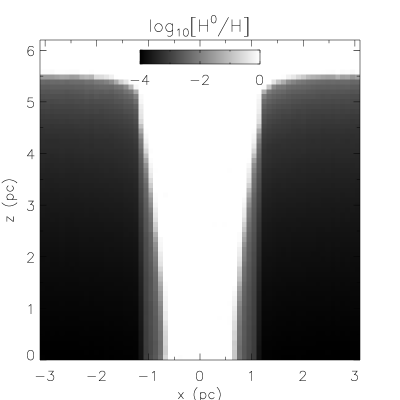
Figure 3: The ionization structure, H⁰/H, of a shadowed region produced by an impervious circular cloud, with ionizing stellar radiation incident from below as described in §8.2.

Figure 4: (a) The nebular temperature, $T(r,z)$, within a region shadowed by a circular cloud that acts as an opaque plate, as shown in Fig. 3. Stellar photons are injected parallel to the $z$ axis (vertical in Fig. 3); $r$ is the radial distance from the axis of the shadow. The radius of the cloud is 1.14 pc. Heavy lines show the case of the benchmark nebular composition, roughly solar; light lines are solar except that there is no helium. Solid lines; $r/R$(cloud) = 1.17; long dashes:, $r/R$(cloud) = 1.01; short dashes:, $r/R$(cloud) = 0.96. The figure shows the dramatic effects that He recombination radiation has on the physical conditions within the shadow (see text), most importantly, the very low $T_{e}$ if there is no He. (b) $T(r,z)$ as a function of $z$ at $r/R$(cloud) = 0.095 pc (solid lines) and $z$ = 2.6 pc (dashed).

Fig. 4(a) shows $T(r,z)$, plotted against $z$, at $r/R_{\rm cloud}$ = 1.17 (solid line), 1.01 (long dashes), and 0.964 (short dashes). The lines terminate when H becomes $>$95% neutral. We see that for the inner no-He model (light short dashes), $T(r/R_{\rm cloud}=0.964$) is much lower than the other temperatures at all $z$, as predicted in Cantó et. al. (1998). H recombination radiation has a mean energy of only $\sim 0.68k_{B}T_{e}$ = 0.4 eV. Photons released during the cascade following He recombinations (mostly the 19.8 eV 2${}^{3}\rm S\rightarrow 1^{1}$S line) can release $\sim(20-13.6)$ eV = 6.3 eV in photoelectric heating with each ionization and penetrate $\sim$3 times as far as H recombinations in the shadow. Thus, the He recombination photons have a major effect on the heating even though there are 10 times as many from H. Even just outside of the shadow (the long dashed curves) the shadow temperature is about the same as far from the cloud (the solid curve), until the He becomes neutral in the gas fully illuminated by the star, at the point of the slight blip at $z\sim$3.9 pc in the heavy solid curve. Outside of the shadow, we see the expected increase of $T(r,z)$ with $z$, showing the effect of hardening the stellar radiation, for both helium- and no-helium models. (Since we did not account for cooling by collisional excitation of H lines, the maximum temperature reached by the no-He model is probably significantly too large.) Within the shadow (short dashes), there is little change of $T$ with $z$ because the spectrum of the ionizing recombination radiation changes little along the axis of the shadow. Within the shadow, $T(z)$ for the He models (heavy short dashes) is significantly less than outside, so the collisionally excited line strengths are appreciably weaker.

Fig. 4(b) shows $T(r,z)$ plotted against $(r/R_{\rm cloud}$) at two values of $z$: solid lines are for $z$ = 0.1 pc; dashed for 2.6 pc. As before, the thick lines are for models with He, the thin for no helium. The inward drop of $T(r)$ at $r=R_{\rm cloud}$ is obvious. We see that the low $T_{e}$ of the no-He models holds at all $r$. There is an increase in $T(r)$ near the center for the helium models because the outer part of the shadow is mainly ionized by the soft recombination photons from H, while the He photons penetrate and deposit more energy when they are absorbed. There is no similar effect for the no-He shadow; all ionizing photons are soft. We see the penetrating power of the He photons into the shadow. Outside the shadow $T(r)$ decreases somewhat with increasing $r$ because the harder diffuse photons can reach the shadow more easily than the softer.

This example shows the importance of diffuse helium radiation in shadow regions and may also help explain why He is less ionized than H in the Diffuse Ionized Gas (Reynolds & Tufte, 1995). It shows that any treatment of the nebular diffuse radiation field inpinging onto shadowed regions must include a careful treatment of the helium recombination radiation. We will investigate this effect and other 3D photoionization models in future papers.

An anonymous referee provided helpful comments. JSM thanks a PPARC Visitors Grant to the University of St. Andrews, KW acknowledges support from a PPARC Advanced Fellowship. We thank Kirk Korista for comments and providing the cloudy benchmark models and Mike Barlow and Barbara Whitney for comments on early versions of the paper. The mocassin tests were carried out on the Enigma SunFire Cluster, at the HiPerSPACE Computing Centre, UCL, which is funded by PPARC.

References

- Aldrovandi & Péquinot (1973) Aldrovandi, S. M. V., & Péquinot, D. 1973, A&A, 25, 137
- Ali et al. (1991) Ali, B.,Blum, R. D., Bumgardner, T. E., Cranmer, S. R., Ferland, G. J., Haefner, R. I., & Tiede, G. P., 1991, PASP, 103, 1182
- (3) Armstrong, J. W., Rickett, B. J., & Spangler, S. R., 1995, ApJ, 443, 209
- Arnaud & Rothenflug (1985) Arnaud, M., & Rothenflug, R.1985, A&AS, 60, 425
- Baessgen, Diesch, & Grewing (1990) Baessgen, M., Diesch, C., & Grewing, M. 1990, A&A, 237, 201
- Benjamin, Skillman, & Smits (1999) Benjamin, R. A., Skillman, E. D., & Smits, D. P. 1999, ApJ, 514,307
- Bjorkman & Wood (2001) Bjorkman, J. E., & Wood, K. 2001, ApJ, 554, 615
- Black (1981) Black, J. H. 1981, MNRAS, 197, 553
- Brocklehurst (1972) Brocklehurst, M. 1972, MNRAS, 157, 211
- Brown & Mathews (1970) Brown, R. L., & Mathews, W. G. 1972, ApJ, 160, 939
- Cantó et. al. (1998) Cantó, J., Raga, A., Steffen, W., & Shapiro, P. R. 1998, ApJ, 502, 695
- Ciardi et al. (2001) Ciardi, B., Ferrara, A., Marri, S., & Raimondo, G. 2001, MNRAS, 324, 381
- Ciardi et al. (2002) Ciardi, B., Bianchi, S., & Ferrara, A. 2002, MNRAS, 331, 463
- Dove & Shull (1994) Dove, J.B., & Shull, J. M. 1994, ApJ, 423, 196
- Dove, Shull, & Ferrara (2000) Dove, J.B., Shull, J. M., & Ferrara, A. 2000, ApJ, 531, 846
- Drake, Victor, & Dalgarno (1969) Drake, G. W. F., Victor, G. A., Dalgarno, A.
- Elmegreen (1997) Elmegreen, B.G. 1997, ApJ, 477, 196
- Elmegreen, Kim, & Staveley-Smith (2001) Elmegreen, B. G., Kim, S., & Staveley-Smith, L., 2001, ApJ, 548, 749
- Ercolano et al. (2003) Ercolano, B., Barlow, M. J., Storey, P. J., & Liu, X.-W. 2003, MNRAS, 340, 1136
- Gruenwald, Viegas, & Broguiere (1997) Gruenwald, R., Viegas, S. M., & Broguiere, D. 1997, ApJ, 480, 283
- Falgarone, Phillips, & Walker (1991) Falgarone, E., Phillips, T. G., & Walker, C. K., 1991, ApJ, 378, 186
- Ferland (1994) Ferland, G. J. 1994, Hazy, University of Kentucky Dept. of Physics and Astronomy Internal Report
- Ferland et al. (1995) Ferland, G. J. et al., 1995, in Williams, R., Livio, M., eds, STScI Symp. 8, “The Analysis of Emission Lines”, Cambridge Univ. Press, Cambridge, p. 83
- Hartmann & Burton (1999) Hartmann, D., & Burton, W. B., 1999, “Atlas of Galactic Neutral Hydrogen”, 1999, VizieR On-line Data Catalog: VIII/54
- Heiles et al. (1996) Heiles, C., Koo, B-C., Levenson, N. A. & Reach, W. T. 1996, ApJ, 462, 326
- Hummer & Storey (1998) Hummer, D. G., & Storey, P.J. 1998, MNRAS, 297, 1073
- Hummer (1994) Hummer, D. G. 1994, MNRAS, 268, 109
- Katz et al. (1996) Katz, N., Weinberg, D. H., & Hernquist, L. 1996, ApJS, 105, 19
- Kingdon & Ferland (1996) Kingdon, J. B., & Ferland, G. J. 1996, ApJS, 106, 205
- Lauroesch, Meyer, & Blades (2000) Lauroesch, J. T., Meyer, D. M., & Blades, J. C. 2000, ApJ, 543, L43
- Lucy (1999) Lucy, L. B., 2003, A&A, 403, 261
- Lucy (1999) Lucy, L. B., 1999, A&A, 344, 282
- Mathis (2000) Mathis, J. S. 2000, ApJ, 544, 347
- Mathis (1976) Mathis, J. S., 1976,ApJ, 207, 442
- Mathis, Whitney, & Wood (2002) Mathis, J. S., Whitney, B. & Wood, K. 2002, ApJ, 574, 812
- Miller & Cox (1993) Miller, W. W., III, & Cox, D. P.1993, ApJ, 417, 579
- Minter & Spangler (1996) Minter, A. H., & Spangler, S. R., 1996, ApJ, 458, 194
- Nussbaumer & Storey (1983) Nussbaumer, H., & Storey, P. J. 1983, A&A, 126, 75
- Nussbaumer & Storey (1984) Nussbaumer, H., & Storey, P. J. 1984, A&AS, 56, 293
- (40) Nussbaumer, H., & Storey, P. J. 1987, A&AS, 69, 123
- Och, Lucy, & Rosa (1998) Och, S. R., Lucy, L. B., & Rosa, M. R. 1998, A&A, 336, 301
- Osterbrock (1989) Osterbrock, D. E. 1989, Astrophysics of Gaseous Nebulae and Active Galactic Nuclei, University Science Books, Mill Valley, CA
- Péquignot et al. (2001) Péquignot, D., et al. 2001, in “Spectroscopic Challenges of Photoionized Plasmas”, G. Ferland & D. W. Savin, eds., ASP Conference Series Vol. 247. San Francisco: Astronomical Society of the Pacific, 533
- Pradhan & Peng (1995) Pradhan, A. K., & Peng, J. 1995, in Space Telescope Science Institute Symposium Series No. 8, Ed: R.E.Williams and M.Livio, Cambridge University Press, p8
- Press et al. (1992) Press, W. H., Teukolsky, S. A., Vetterling, W. T., & Flannery, B. P. 1992, Numerical Recipes in C++ (2d ed.; New York: Cambridge Univ. Press)
- Reynolds & Tufte (1995) Reynolds, R. J., & Tufte, S. L. 1995, ApJ, 448, 715
- Reynolds, Haffner, & Madsen (2002) Reynolds, R. J., Haffner, L. M., & Madsen, G. J., 2002, in “Galaxies: the Third Dimension”, M. Rosada, L. Binette, & L. Arias, eds. (Astr. Soc. Pacific,: San Francisco)
- Reynolds, Haffner, & Tufte (1999) Reynolds, R. J., Haffner, L. M., & Tufte, S.L. 1999, ApJ, 525, L21
- Savage & Sembach (1996) Savage, B. D., & Sembach, K. R. 1996, ARAA, 34, 279
- Seaton (1959) Seaton, M. J. 1959, MNRAS, 119, 81
- Simon et al. (2001) Simon, R., Jackson, J. M., Clemens, D. P., & Bania, T. M. 2001, ApJ, 551, 747
- Spaans (1996) Spaans, M., 1996, A&A, 307, 271
- Spitzer (1978) Spitzer, L. 1978, Physical Processes in the Interstellar Medium, New York, Wiley
- Stanimirović & Lazarian (2001) Stanimirović, S. & Lazarian, A. 2001, ApJ, 551, L53
- Stasińska (2002) Stasińska, G., 2002, lectures at the XIII Canary Islands Winterschool on Cosmochemistry, astro-ph/0207500
- Storey & Hummer (1995) Storey, P. J., & Hummer, D. G. 1995, MNRAS, 272, 41
- Van Blerkom & Arny (1972) Van Blerkom, D., & Arny, T. T. 1972, MNRAS,156, 91
- Verner & Ferland (1996) Verner, D. A, & Ferland, G. J. 1996, ApJS, 103, 467
- (59) Verner, D. A., Ferland, G. J., Korista, K. T., & Yakovlev, D. G. 1996, ApJ, 465, 487
- Wood & Loeb (2000) Wood, K., & Loeb, A. 2000, ApJ, 545, 86